Do DJIA Firms Reflect Stationary Debt Ratios? - MDPI
←
→
Page content transcription
If your browser does not render page correctly, please read the page content below
economies
Article
Do DJIA Firms Reflect Stationary Debt Ratios?
Feng-Li Lin
 Department of Accounting, Chaoyang University of Technology, Taichung 413310, Taiwan;
 bonnie@gm.cyut.edu.tw; Tel.: +886-4-2332-3000 (ext. 4580)

 Received: 18 July 2020; Accepted: 15 September 2020; Published: 28 September 2020

 Abstract: To form optimum firm capital structure strategies to face unanticipated economic events,
 firm managers should understand the stability of a firm’s capital structure. The aim of this research
 was to study whether the debt ratio is stationary in listed firms on the Dow Jones Industrial Average
 (DJIA). Two vital capital structure concepts regarding pecking order and trade-off theory are fairly
 contradictory. Using opposing theoretical contexts, the Sequential Panel Selection Method apparently
 categorizes which and how many series are stationary processes in the panel. This method was used
 to test the mean reverting properties of the 25 companies listed on Dow Jones Industrial Average
 between 2001 and 2017 in this study, which is expected to fill the current gap in the literature.
 The overall results show that stationary debt ratios exist in 10 of the 25 studied firms, supporting the
 trade-off theory. Moreover, the 10 firms utilizing trade-off theory are affected by firm size, profitability,
 growth opportunity, and dividend payout ratio. These results provide vital information for firms to
 certify strategies to optimize capital structure.

 Keywords: debt ratio; trade-off theory; Sequential Panel Selection Method; stationarity

 JEL Classification: C32; F31

1. Introduction
      The Dow Jones Industrial Average (DJIA) represents 30 of the most highly influential as well
as capitalized firms in the US economy. Examining the capital structure of these firms restrains
their capability to manage external combative circumstances (Abor 2005), with each firm requiring
optimization of the capital structure regarding financial system stability. To form an optimum firm
capital structure policy to deal with unanticipated economic events, firm managers ought to understand
the stability of a firm’s capital structure. The aim of this research was to study whether debt ratios are
stationary in listed firms on the DJIA.
      Two major theories describing the corporate capital structure are pecking order and trade-off
theory, with Modigliani and Miller (1958) offering optimal capital structures replicating both with
debtless, default-cost tax advantages. As a trade-off between interest tax shields and financial distress
costs (Miller 1977; Leland 1994; Brealey and Myers 2003; Frank and Goyal 2009), trade-off theory
sustains the occurrence of an optimal debt ratio to maximize firm value; this static theory predicts
reversion of the factual debt ratio to an optimal or objective value. In terms of the pecking order
theory, no definite optimal debt ratio is obvious because of information asymmetry costs. Following
the financing hierarchy, companies utilize less risky debt prior to risky external equity financing while
favoring internal financing (retained earnings) over other sources, e.g., issuing and debt security
(Myers and Majluf 1984; Myers 1984).
      The trade-off concept was previously studied at a quantitative level as well as in terms of
speediness of adjusting company debt ratios to the assumed target. DeAngelo and Roll (2015) utilized
a time-varying target approach to study inter-firm variation, with a 15,096-industrial-firm sample

Economies 2020, 8, 76; doi:10.3390/economies8040076                           www.mdpi.com/journal/economies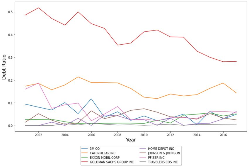
Economies 2020, 8, 76                                                                                2 of 19

from CRSP/Compustat files between 1950 and 2008. Capital structure stability was observed to be
uncommon and occurring mainly at low leverage; overall, it was shown to be essentially interim,
with several firms discarding low leverage during post-war economic expansion. Nehrebecka and
Dzik-Walczak (2018) presented a meta-study on 187 regressions from 33 papers regarding leverage
and leverage adaptions in Polish listed firms between 1998 and 2015, thereby verifying publication
selection bias. Polish listed firms were shown to alter present leverage levels to the yearly optimum
rate of 41.55%, thereby requiring 1.3 years to lessen the half-distance to achieve optimum leverage.
Compared with outcomes presented by other researchers, this was a rather high adjustment rate.
Judging from a partial adjustment model assessed via the GMM estimation procedure utilizing
information regarding an unbalanced 390-UK-firm panel between 1984 and 1996, Ozkan (2001) showed
the target capital structure occurrence and indicated a yearly 43% adjustment rate for these firms.
Flannery and Rangan (2006) discussed the existence of the target capital structure and specified 33%
and 34% adjustment rates for Compustat firms and the US, respectively. Elsas and Florysiak (2011)
indicated a 26% adjustment rate for all Compustat firms.
      Much previous research in this field supports the static trade-off theory (Solomon 1963;
Shyam-Sunder and Myers 1999; Hovakimian et al. 2001; Ozkan 2001; Sogorb Mira and López-Gracia
2003; Leary and Roberts 2005; Flannery and Rangan 2006; Hackbarth et al. 2007; Chang and Yu 2010;
Elsas and Florysiak 2011; Chen et al. 2019; and Dierker et al. 2019). In contrast, other studies do not
support the trade-off concept, for example, Fama and French (2002); Banerjee et al. (2004); Christopher
and Tong (2005); Ju et al. (2005); Botta (2019); Jarallah et al. (2019); and Chen et al. (2019). Empirical
evidence of trade-off theory (stationarity) is abundant, however, a crucial point worth noting is that
structural breaks are generally not considered in any prior studies. By identifying the structural change
points, specific economic factors resulting in debt ratios fluctuating significantly in individual firms
during the sample period can be analyzed.
      The motivation for this study was to determine whether shock economic events relevant to
time–debt ratio paths are permanent or temporary, as seen from 425 firm-year observations listed on
the DJIA from 2001 to 2017. These DJIA samples can be treated as representatives for verification of
firm finance trade-off theory in that the 30-stock index is considered to serve as a proxy for the health
of the wider US economy, being one of the most cited financial barometers in the world (Paul 2019).
Whether or not debt ratios are characterized by a unit root has important policy implications. If debt
ratios are an I (0) stationary process, then any shock effect is temporary. Moreover, diverting the debt
ratios from one level to another would return the ratio to its original stability level. Thus, controlling
the trend path or mean value in the long run is critical.
      There are several contributions to this study. First, to the best of our knowledge, this study is the
first to utilize the panel unit root test from Kapetanios, Snell, and Shin (Kapetanios et al. 2003) with a
critical target for firm managers rather than simply using a temporary strategy in the short run. We use
the Fourier function via the Sequential Panel Selection Method (SPSM) process to study the astringent
debt ratio of listed firms on the DJIA. In contradiction to panel-based unit root tests (PURTs) that
involve a-unit root allied testing for whole units in the panel and that are incapable of deciding I (0)
and I (1) series mixtures, the SPSM, proposed by Chortareas and Kapetanios (2009), divides an entire
panel into sets of nonstationary and stationary series, respectively, to classify which and how many
series are stationary procedures of the panel. Secondly, the debt ratios of various firms are renowned
to be contemporaneously correlated since independence is considered to be a realistic presumption.
To check for any cross-section dependency among the data sets, we approximate the tests’ bootstrap
distribution, which was not previously attempted, assuming that the individuals are cross-section
independent. Hence, our study is expected to fill the current gap in the literature. The overall panel
test results show that 10 of the 25 studied companies (40%) have stationary debt, i.e., 10 firms support
the trade-off theory, consistent with previous findings regarding company profitability, size, market
value (growth opportunity), and dividend payout ratio. The outcomes of this study demonstrate vital
policy applications for managers in the US.
Economies 2020, 8, 76                                                                                      3 of 19

   This research work is classified according the following sections: Section 2 presents the empirical
model and sample, Section 3 displays the empirical results, and Section 4 presents the conclusions.

2. Data and Empirical Model

2.1. Data
     The yearly sample panel covered all the firms listed on the Dow Jones Industrial Average (DJIA)
between 2001 and 2017 employed in this study. Data were extracted from the yearly Compustat files.
After exclusion of five firms with missing continuous data from 2001 to 2017, the final sample consisted
of 25 publicly traded companies listed on the DJIA (namely, 3M Co., American Express Co., Boeing
Co., Caterpillar Inc., Chevron Corp., Coca-Cola Co., Disney (Walt) Co., DowDuPont Inc., Exxon Mobil
Corp., Goldman Sachs Group Inc., Home Depot Inc., Intel Corp., Intl Business Machines Corp., Johnson
& Johnson, JPMorgan Chase & Co., McDonald’s Corp., Merck & Co., Nike Inc-Club, Pfizer Inc., Procter
& Gamble Co., Travelers Cos Inc., United Technologies Corp., Verizon Communications Inc., Walgreens
Boots Alliance Inc., and Walmart Inc.).

2.2. Empirical Model
      Several studies indicated that panel-based unit root tests (PURTs) and conventional tests with
and without nonlinearities can be used for accounting, macroeconomics, and financial purposes.
In addition, the ADF (Augmented Dickey-Fuller) unit root test uses almost less power to find a mean
reversion trend for the series. Although the nonlinear modification finding unnecessarily indicated
nonlinear mean reversion, stationarity tests via a nonlinear system were employed.
      A nonlinear PURT is employed by Ucar and Omay (2009) and in a nonlinear context in Kapetanios,
Snell, and Shin (Kapetanios et al. 2003, KSS) according to the PURT process designed by Im et al. (2003),
thereby verifying the time-series data mean reversion. Perron (1989) proposed that the power to refuse
a unit root reduces if a structural break is neglected; further, the stationary alternative becomes true if a
structural break occurs. Furthermore, structural fluctuations occur in a sample-producing procedure,
although these were later disregarded, with the investigation switched toward an a-unit root null
assumption. Hence, Chortareas and Kapetanios (2009) suggested mixing the SPSM with the KSS
PURTs, with the Fourier function employed to estimate the mean reverting properties for 25 companies
listed on the DJIA between 2001 and 2017.
      In agreement with previous research, KSS PURT is used here to identify the occurrence of
nonstationarity in contradiction with a nonlinear but wholly stationary exponential smooth transition
autoregressive (ESTAR) procedure. The equation is as follows:
                                                 n                    o
                                ∆Debtt = γDebtt−1 1 − exp(−θDebt2t−1 ) + νt                                   (1)

where Debtt is the ratio of total liabilities to total assets, vt defines an i.i.d. error with constant adjustment
as well as nil mean, and θ ≥ 0 represents the ESTAR procedure transition variable for controlling the
transition rate. Debtt abides by a PURT for the null hypothesis, but a nonlinear stationary ESTAR for
the substitute. A weakness of such basis is the variable γ, which is unidentified for the null assumption.
Kapetanios et al. (2003) utilize the 1st-order Taylor series estimation on {1 − exp(−θDebt2t−1 )} regarding
the null hypothesis θ = 0. The resulting estimated Formula (1) via supplementary expression is
therefore as follows:
                                                               X k
                                ∆Debtt = ξ + δDebt3t−1 +           θi ∆Debtt−i + νt                            (2)
                                                             i=1

These alternative and null assumptions on this basis are specified as δ = 0 in contradiction of δ < 0.
A nonlinear PURT via regression [1] is extended by Ucar and Omay (2009), with the equation being

                             ∆Debti,t = γi Debti,t−1 {1 − exp(−θi Debt2i,t−1 )} + νi,t                        (3)
Economies 2020, 8, 76                                                                                                     4 of 19

     Ucar and Omay (2009) employ the first-order Taylor formula estimation to Equation (1) if θi = 0
for whole i, resulting in the following supplementary equation:

                                                                      k
                                                                      X
                            ∆Debti,t = ξi + δi Debt3i,t−1 +                 θi,j ∆Debti,t− j + νi,t                          (4)
                                                                      j=1

where δi = θi γi . The hypotheses developed for PURT via regression (4) are shown as:

                          H0 : δi = 0, regarding whole i, (linear nonstationarity);
                                                                                                                             (5)
                          H0 : δi < 0, regarding certain i, (nonlinear stationarity).

      Moreover, SPSM with the KSS PURT and the Fourier function is represented by

                                                  k1
                                  3
                                                  X                                    2πkt               2πkt
            ∆Debti,t = ξi + δi Debt   i,t−1   +         θi,j ∆Debti,t− j + ai,1 sin(        ) + bi,1 cos(      ) + εi,t      (6)
                                                                                        T                  T
                                                  j=1

where t = 1, 2, 3, . . . T and normal regarding choosing [sin(2πkt/T), cos(2πkt/T)] under the Fourier
equation are able to unconditionally approximate the accuracy level according to the integrable
equation. If k denotes the frequency chosen for the estimation, [ai ,bj ]’ estimates this frequency
element amplitude and displacement, displaying no less than one frequency element existing for the
structural break. Gallant (1981); Becker et al. (2004), as well as Enders and Lee (2012), indicated that
Fourier estimation enables catching an unidentified behavior despite its unperiodical process. Without
previous information regarding the data-break shape, a grid-pursuit is initially completed to discover
the optimal frequency.
      Although there are two significant capital structure concepts of pecking order and trade-off theory
that contradict each other, the SPSM in this study is employed for both opposing theoretical contexts,
seemingly classifying which and how many series are stationary processes in the panel. This is carried
out via KSS PURT to test time-series mean reverting properties, such as the debt ratios of the 25 firms
listed on the DJIA from 2001 to 2017. Relevant advantages of this model include:

(1)   The flexibility and power to detect mean reversion trend for the series;
(2)   Classification of the whole panel into two group series, i.e., stationary and
      nonstationary, respectively;
(3)   Clear identification of how many and which series in the panel are stationary processes;
(4)   Use of stationarity tests based on a nonlinear framework for the nonlinear adjustment of economic
      variables because of the cycle and government policy implementation.

      The SPSM flowchart in Figure 1 shows the following:

(1)   KSS PURTs with a Fourier function are associated with the whole panel debt ratio. The process
      discontinues and whole panel series are not stationary, therefore, the null assumption is not
      refused. Step 2 is initiated if the null is refused;
(2)   The series is removed via the minimum KSS statistic due to its classified stationarity;
(3)   The first step is returned to in case of the rest of the series, otherwise, the process is stopped with
      the whole panel-disconnected series.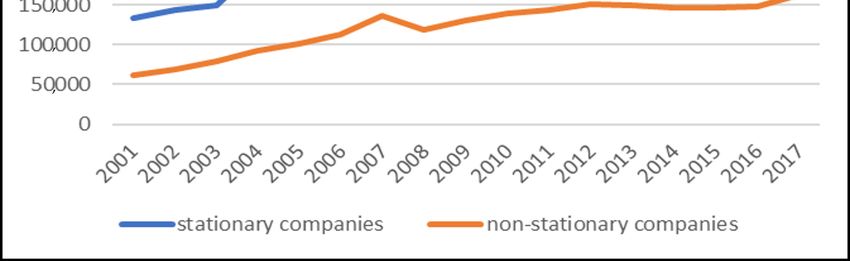
Economies 2020, 8, 76                                                                              5 of 19
Figure 1

                        Figure 1. Sequential Panel Selection Method (SPSM) flowchart.

      The final outcome is a separation of all panels into groups of nonstationary and stationary series.

3. Empirical Results

3.1. Results
     Table 1 displays the annual debt ratio description statistics in each company regarding panel
samples from 2001 to 2017. The total number of firms is 25, with 425 firm-year observations. Except for
McDonald’s Corp., the debt ratio is non-normally distributed for all firms, according to the Jarque–Bera
(J–B) statistics results. Some traditional unit root tests, e.g., the ADF, PP (Phillips and Perron 1988);
and KPSS (Kwiatkowski et al. 1992), were initially carried out.
     Some univariate unit root and PURTs were carried out. Table 2 indicates the outcomes of the ADF,
PP, and KPSS unit root tests for debt ratio, proposing that the debt ratios of nine firms (i.e., Chevron
Corp., Disney (Walt) Co., Exxon Mobil Corp., Goldman Sachs Group Inc., Intel Corp., McDonald’s
Corp., Merck & Co., Verizon Communications Inc., and Walmart Inc.) were all non-stationary in
univariate unit root tests in terms of constants and trend. Two firms (i.e., American Express Co. and
JPMorgan Chase & Co.) with nonstationary constants and trend changed to stationary in the first
instance. Whichever other firms’ unit root tests were chosen, their ADF, PP, and KPSS unit root test
outcomes for debt ratio generated ambiguous outcomes.

                                                      1
Economies 2020, 8, 76                                                                                                                                                  6 of 19

                                                                Table 1. Summary statistics of the debt ratio.

                        Companies                      Mean               Max.              Min.            Std.Dev.           Skew.              Kurt.      J-B
              3M CO.                                    0.217             0.369             0.119             0.073            0.994              2.922     2.807
              AMERICAN EXPRESS CO.                      0.375             0.548             0.227             0.094            −0.074             2.066     0.633
              BOEING CO.                                0.172             0.275             0.091             0.061            0.508              1.979     1.468
              CATERPILLAR INC.                          0.498             0.547             0.425             0.043            −0.306             1.517     1.823
              CHEVRON CORP.                             0.110             0.225             0.048             0.058            0.620              2.145     1.605
              COCA-COLA CO.                             0.317             0.543             0.153             0.128            0.519              1.822     1.748
              DISNEY (WALT) CO.                         0.225             0.289             0.179             0.034            0.225              1.910     0.984
              DOWDUPONT INC.                            0.274             0.342             0.177             0.049            −0.429             2.234     0.937
              EXXON MOBIL CORP.                         0.064             0.129             0.035             0.031            1.044              2.737     3.140
              GOLDMAN SACHS GROUP INC.                  0.584             0.641             0.510             0.041            −0.510             2.056     1.368
              HOME DEPOT INC.                           0.267             0.607             0.040             0.180            0.348              2.165     0.836
              INTEL CORP.                               0.092             0.223             0.019             0.076            0.712              1.886     2.316
              INTL BUSINESS MACHINES CORP.              0.285             0.374             0.210             0.054            0.176              1.794     1.117
              JOHNSON & JOHNSON                         0.128             0.220             0.046             0.048            −0.032             2.356     0.296
              JPMORGAN CHASE & CO.                      0.250             0.317             0.195             0.039            0.265              1.769     1.273
              MCDONALD’S CORP.                          0.440             0.874             0.291             0.173            1.759              4.647   10.684 ***
              MERCK & CO.                               0.190             0.278             0.119             0.046            0.507              2.260     1.115
              NIKE INC-CLUB                             0.087             0.172             0.025             0.046            0.724              2.371     1.764
              PFIZER INC.                               0.192             0.255             0.069             0.054            −0.800             2.556     1.955
              PROCTER & GAMBLE CO.                      0.280             0.395             0.225             0.056            0.886              2.314     2.556
              TRAVELERS COS INC.                        0.058             0.064             0.041             0.006            −1.048             3.542     3.322
              UNITED TECHNOLOGIES CORP.                 0.198             0.284             0.140             0.042            0.698              2.304     1.722
              VERIZON COMMUNICATIONS INC.               0.307             0.487             0.167             0.101            0.543              1.940     1.632
              WALGREENS BOOTS ALLIANCE INC.             0.098             0.262             0.001             0.077             0.590             2.355     1.280
              WALMART INC.                              0.259             0.281             0.227             0.016            −0.556             2.393     1.137
                                Note: The sample period is from 2001 to 2017. *** indicates significance at the 5% and 1% levels, respectively.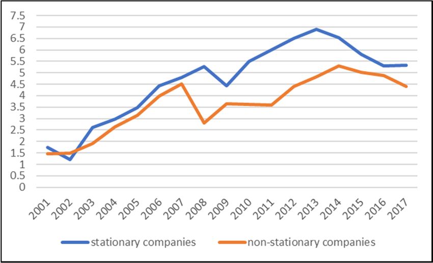
Economies 2020, 8, 76                                                                                                                                                                                      7 of 19

                                                                    Table 2. Univariate unit root tests with constants and trend.

                                                                                             Level                                                      1st Difference
                                                                        ADF                    PP                 KPSS                  ADF                   PP                  KPSS
                   3M CO.                                             −2.732(2)            −1.265(0)             0.114[2]             −3.096(0)            −3.129(1)             0.062(1)
                   AMERICAN EXPRESS CO.                              −5.745(3) **          −1.097(1)            0.157[2] **         −4.002(0) **         −4.024(1) **            0.076(0)
                   BOEING CO.                                        −3.613(3) *           −2.028(2)            0.124[0] *           −3.581(0) *         −4.739(6) ***         0.231(5) ***
                   CATERPILLAR INC.                                   −2.726(3)            −2.028(2)             0.107[1]             −3.389(1)           −3.278(11)           0.261[8] ***
                   CHEVRON CORP.                                      −1.286(2)            −1.555(5)            0.177[2] **           −2.178(1)            −1.876(4)           0.185[5] **
                   COCA-COLA CO.                                     −5.75(3) ***         −3.541(15) *          0.166[2] **         −3.874(0) **         −3.939(6) **         0.500[15] ***
                   DISNEY (WALT) CO.                                  −1.215(0)            −1.587(1)            0.142[1] *          −4.663(0) ***        −4.877(3) ***         0.147[1] **
                   DOWDUPONT INC.                                     −2.681(2)            −1.550(1)             0.085[2]             −2.693(2)            −2.502(1)             0.103[1]
                   EXXON MOBIL CORP.                                  −1.403(0)            −1.381(2)            0.169[2] **           −3.202(0)            −2.842(4)           0.161[4] **
                   GOLDMAN SACHS GROUP INC.                           −2.834(0)            −2.821(3)            0.144[1] **         −3.801(0) **         −4.621(5) ***        0.296[10] ***
                   HOME DEPOT INC.                                    −2.677(1)            −1.734(1)             0.087[2]             −2.400(0)            −2.396(2)             0.094[0]
                   INTEL CORP.                                        −1.993(0)            −1.996(12)           0.163[2] **         −4.730(1) ***       −5.001(13) ***        0.394[12] ***
                   INTL BUSINESS MACHINES CORP.                      −3.398(1) *          −4.006(7) **          0.137[1] *           −3.503(1) *         −4.186(14) **         0.216[5] **
                   JOHNSON & JOHNSON                                  −3.164(1)            −1.686(0)             0.067[1]             −2.903(0)            −2.903(0)             0.073[1]
                   JPMORGAN CHASE & CO.                               −2.347(2)            −1.832(1)             0.100[2]            −3.270(0) *          −3.333(1) *            0.082[0]
                   MCDONALD’S CORP.                                    0.376(2)             0.616(4)            0.163[2] **          −3.652(1) *           −3.081(7)             0.115[3]
                   MERCK & CO.                                        −1.770(0)            −1.741(6)            0.176[2] **         −4.616(0) ***       −8.472(14) ***        0.500[15] ***
                   NIKE INC-CLUB                                       0.019(3)            −0.987(15)            0.183[2]           −6.111(2) ***        −8.907(8) ***         0.302[8] ***
                   PFIZER INC.                                       −3.679(3) *           −2.387(3)            0.123[1] *          −4.660(0) ***        −4.602(1) ***         0.187[6] **
                   PROCTER & GAMBLE CO.                               −2.083(0)            −2.022(2)             0.149[1]           −3.998(1) **        −8.487(13) ***        0.469[14] ***
                   TRAVELERS COS INC.                               −4.999(0) ***        −4.999(0) ***           0.099[3]           −7.270(0) ***       −16.669(14) ***       0.500[15] ***
                   UNITED TECHNOLOGIES CORP.                         −3.394(0) *          −3.535(8) *           0.155[2] **         −4.809(2) ***       −12.878(11) ***       0.500[15] ***
                   VERIZON COMMUNICATIONS INC.                        −2.134(0)            −2.570(8)            0.163[2] **          −3.524(1) *         −3.506(12) *          0.228{8} ***
                   WALGREENS BOOTS ALLIANCE INC.                      −2.904(2)          −8.148(13) ***         0.153[3] **         −7.117(1) ***        −4.954(7) ***         0.235[9] ***
                   WALMART INC.                                       −2.521(0)            −2.521(0)            0.141[1] **         −5.883(0) ***        −7.958(5) ***        0.500[15] ***
      Note: ***, ** and * indicate significance at the 0.01, 0.05, and 0.1 levels, respectively. The numbers in parentheses indicate the lag order selected based on the recursive t-statistic, as suggested
      by Perron (1989). The numbers in the brackets indicate truncation for the Bartlett Kernel, as suggested by the Newey–West test (1987).
Economies 2020, 8, 76                                                                                                           8 of 19

     In Table 3, three of the first-generation PURTs were adopted; their relevant outcomes showed
that Levin et al. (2002) and Im et al.’s (2003) unit root tests for debt ratio results were stationary
in contrast with Maddala and Wu’s (1999) nonstationary testing results. However, this major first
generation PURT advantage is the hypothesis of cross-sectional independence crosswise data. Without
contemplating simultaneous connections among data, the PURT is biased toward refusing the joint unit
root assumption. Cross-sectional dependencies are recognized in second-generation PURTs, suggesting
a greater method to estimate the debt ratios. Four second-generation PURTs (Bai and Ng 2004; Moon
and Perron 2004; Choi 2002; and Pesaran 2007) were used for this study.

                                       Table 3. Panel unit root tests (first generation).

                                                t∗ρ               ρ̂               t∗B
                                                                                    ρ               t∗C
                                                                                                     ρ
             Levin et al. (2002)
                                              10.059         −0.333 ***          10.965           16.755
                                              (1.000)         (0.001)            (1.000)          (1.000)
                                             t_barNT           Wt,bar             Zt,bar          t_barDF
                                                                                                       NT
                                                                                                                    ZDF
                                                                                                                     t,bar
               Im et al. (2003)
                                              −2.042            0.591          −2.748 ***         −2.048         −2.778 ***
                                                               (0.723)          (0.003)                           (0.003)
                                               PMW              ZMW
         Maddala and Wu (1999)
                                              46.049           −0.395
                                              (0.633)          (0.654)
      Notes: Levin et al. (2002): t∗p specifies the modified t-statistic calculated via the Bartlett kernel function and a common
      lag truncation variable achieved using K = 3.21T1/3 (Levin et al. 2002). Relevant p-values are in parentheses. ρ̂ is
      the pooled least squares estimator. Relevant standard error values are in parentheses. t∗B     p represents the modified
      t-statistic calculated via the Bartlett kernel function and separate bandwidth variables (Newey and West 1994).
      t∗C
       p indicates the modified t-statistic calculated via a quadratic spectral kernel function and separate bandwidth
      parameters. Lastly, t∗ρ means the modified t-statistic calculated via the Bartlett kernel function and a common
      lag truncation parameter. Relevant p-values are in parentheses. * indicates significance at the 5% level. Im et
      al. (2003): t_barDF
                        NT
                            (respectively t_barNT ) specifies the mean of Dickey Fuller (respectively, Augmented Dickey
      Fuller) individual statistics. ZDF
                                       t,bar
                                             is the standardized t_barDF
                                                                      NT
                                                                         statistic, with relevant p-values in parentheses. Zt,bar
      is the standardized t_barNT statistic based on Dickey Fuller distribution. Wt,bar specifies the standardized t_barNT
      statistic via simulated approximated moments (Im et al. 2003, Table 3). Corresponding p-values are in parentheses.
      * shows significance
                   P          at the 5% level. Maddala and Wu (1999): PMW specifies the Fisher’s test statistic defined as
      PMW = −2 log(pi ), where pi are the p-values from the ADF unit root tests for each cross-section. Under H0 , PMW
      has χ2 distribution with 2N of freedom, where T is infinite and N is fixed. ZMW is the standardized statistic utilized
      for big N samples. Under H0, ZMW has an N (0, 1) distribution, with T and N being infinite.

      Table 4 indicates the results of Moon and Perron (2004), who proposed that debt ratio is stationary.
However, considering our three findings of second-generation PURTs as evidence contradicting
trade-off theory, only one supports trade-off theory. Due to the outcomes of second-generation PURTs
being inconsistent, the SPSM procedure besides the KSS PURT was carried out to ratify debt ratio in
this study.
      As mentioned earlier, PURTs that are a-unit root allied testing for whole panel units are incapable
of deciding (0) and I (1) series mixtures. Therefore, an SPSM course via KSS PURT was used to identify
which and how many series are stationary procedures in the panel.
      Table 5 specifies the outcomes of the KSS PURT trends without Fourier functions of the 25
firms, including the order for KSS PURTs of bootstrap p-values, specific minimum KSS statistics,
and stationary series recognized via the process. Furthermore, when the KSS PURT was initially
used for the entire panels described in Table 5, OU statistics were generated using a PURT value of
2.1923, indicating a p-value at 1% significance. By subsequently applying the SPSM process, Verizon
Communications Inc. was revealed to be stationary with a value of −3.8103; it was then excluded in
the panel. KSS PURT was reused for the rest of the series. KSS PURT still rejected the null with a
value of −2.1249; Travelers Cos Inc. became stationary here, as the minimum KSS value was −3.7087.
Travelers Cos Inc. was then eliminated in the panel, with KSS PURT reused for the rest of the series.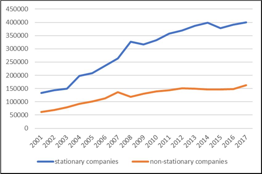
Economies 2020, 8, 76                                                                                                           9 of 19

                                     Table 4. Panel unit root tests (second generation).

                                                 r̂              Zcê              Pcê            MQc              MQ f
             Bai and Ng (2004)
                                                4.0             0.482            54.824              3                4
                                                               (0.315)           (0.297)
                                                t∗a               t∗b             ρ̂∗pool           t∗B
                                                                                                     a               t∗B
                                                                                                                      b
         Moon and Perron (2004)
                                            −10.29 ***       −5.964 ***           0.777         −9.487 ***       −5.824 ***
                                             (0.000)          (0.000)                            (0.000)          (0.000)
                                                Pm                Z                L∗
                 Choi (2002)
                                             −0.077             0.349             0.571
                                             (0.531)           (0.637)           (0.716)
                                                P∗              CIPS             CIPS∗
                Pesaran (2007)
                                                 2             −1.747            −1.747
                                                               (0.460)           (0.460)
      Notes: Bai and Ng (2004): r̂ is the calculated common factor number via IC criteria functions. Pcê is a Fisher’s
      type statistic via p-values of the individual ADF tests. Zcê is a standardized Choi’s type statistic for big N samples.
      p-values are in parentheses. The first computed value r̂1 comes from the filtered test MQ f and the second comes
      from the rectified test MQc . * denotes significance at the 5% level. Moon and Perron (2004): t∗a and t∗b are the unit
      root test statistics obtained via defactored panel data (Moon and Perron 2004). Relevant p-values are in parentheses.
      ρ̂∗pool is the rectified pooled estimate of the autoregressive variable. t∗B     ∗B
                                                                                a and tb are calculated using the Bartlett kernel
      function according to a quadratic spectral kernel function. Choi (2002): The Pm test is an adjusted Fisher’s inverse
      chi-square test (Choi 2001). The Z test is an inverse normal test. The L∗ test is an adjusted logit test. P-values are in
      parentheses. Pesaran (2007): CIPS is the mean of individual cross-sectionally augmented ADF statistics (CADF).
      CIPS∗ denotes the mean of truncated individual CADF statistics. Relevant p-values are in parentheses. P∗ specifies
      the nearest integer of the mean of individual lag lengths obtained from ADF tests.

                        Table 5. Results of panel KSS test with trend and without Fourier function.

       Sequence           OU Statistic           Min. KSS Statistic                                Series
            1           −2.1923 (0.0000)               −3.8103                 VERIZON COMMUNICATIONS INC
            2           −2.1249 (0.0000)               −3.7087                        TRAVELERS COS INC.
            3           −2.0560 (0.0000)               −3.6905                     JPMORGAN CHASE & CO.
            4           −1.9817 (0.0000)               −3.5692                     PROCTER & GAMBLE CO.
            5           −1.9061 (0.0004)               −3.4705                       JOHNSON & JOHNSON
            6           −1.8279 (0.0002)               −3.4109                 WALGREENS BOOTS ALLIANCE INC
            7           −1.7446 (0.0002)               −2.9576                          CHEVRON CORP.
            8           −1.6772 (0.0008)               −2.7664                  INTL BUSINESS MACHINES CORP
            9           −1.6131 (0.0004)               −2.6667                        EXXON MOBIL CORP.
           10           −1.5473 (0.0020)               −2.4373                        MCDONALD’S CORP.
           11           −1.4879 (0.0094)               −2.1723                   GOLDMAN SACHS GROUP INC.
           12           −1.4390 (0.0022)               −2.1411                   UNITED TECHNOLOGIES CORP.
           13           −1.3850 (0.0114)               −2.1392                            INTEL CORP.
           14           −1.3222 (0.0336)               −2.1057                          COCA-COLA CO.
           15           −1.2510 (0.1056)               −1.828                             PFIZER INC.
           16           −1.1933 (0.1580)               −1.8243                            MERCK & CO.
           17           −1.1231 (0.3002)               −1.7788                           NIKE INC-CLUB
           18           −1.0412 (0.4726)               −1.7505                      AMERICAN EXPRESS CO.
           19           −0.9399 (0.4806)               −1.6941                           WALMART INC.
           20           −0.8141(0.6098)                −1.3689                         CATERPILLAR INC.
           21           −0.7032 (0.5528)               −1.1822                         DOWDUPONT INC.
           22           −0.5835 (0.5634)               −1.1095                               3M CO.
           23           −0.4081 (0.7492)               −0.5161                             BOEING CO.
           24           −0.3541 (0.4586)               −0.3554                         HOME DEPOT INC.
           25           −0.3529 (0.4456)               −0.3529                         DISNEY (WALT) CO.
      Notes: OU statistic is the invariant average KSS statistic. Entries in parentheses stand for the asymptotic p-value.
      The significance level is 10%. The maximum lag is 1.

     This process remained until the KSS PURT was unable to refuse the null assumption at 10%
significance, and the process finally discontinued during order 15, when the debt ratios for 15 companies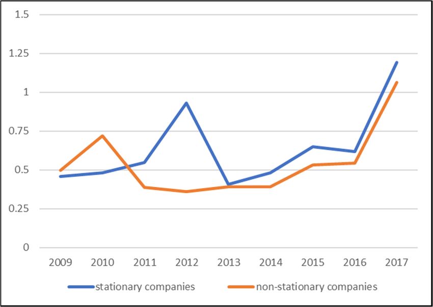
Economies 2020, 8, 76 10 of 19
(i.e., Verizon Communications Inc., Travelers Cos Inc., JPMorgan Chase & Co., Procter & Gamble
CO., Johnson & Johnson, Walgreens Boots Alliance Inc., Chevron Corp., Intl Business Machines Corp.,
Exxon Mobil Corp., McDonald’s Corp., Goldman Sachs Group Inc. and United Technologies Corp.,
Intel Corp., Coca-Cola Co., and Pfizer Inc.) were excluded from the panel. To estimate the robustness
of the testing, the procedure continued until the last sequence.
The KSS PURT statistic is incapable of rejecting the null assumption for whole orders. Ostensibly,
the SPSM process via KSS PURT with trends and without Fourier function offers some evidence
regarding long-term debt-ratio stationarity. As mentioned earlier, Fourier approximation is used
to evaluate structural break likelihood to analyze unidentified behaviors despite the unperiodical
method (Enders and Lee 2009). Thus, KSS PURT with Fourier function was carried out as follows.
First, without previous information regarding the data-break shape, a grid-pursuit was completed
to discover the optimal frequency. Equation (6) was used for every number of k = 1, . . . 5, as per the
suggestions of Enders and Lee (2012), where a sole frequency seized an extensive diversity of breaks.
The residual sum of squares (RSS) specified the sole frequency as k = 2, which was carried out the most
in the whole series.
Table 6 reveals the outcomes of KSS PURT with both trends and Fourier function regarding debt
ratios, where a given order for KSS PURT bootstrap p-values in the lessened panel represented each
minimum KSS statistic; the stationary series was found via the process every time. Table 6 shows that
the unit root null assumption for debt ratio was excluded after KSS PURT with both trend and Fourier
function, which was initially used for the entire panel, generating a value of −3.0469 (1% p-value
significance). Via the SPSM process, Verizon Communications Inc. was found to be stationary for a
panel minimum KSS amount of −3.8103. Meanwhile, Verizon Communications Inc. was eliminated
while the KSS PURT was reused in the rest series. The KSS PURT was then observed to be discarded;
before the unit root null reached a value of −2.9080, Travelers Cos Inc. became stationary for a panel
minimum KSS value of −3.7087, and was also excluded from the panel while KSS PURT was reused
for the rest of the series. In addition, KSS PURT was shown to be discarded before the unit root null
at a value of −2.5176, where Procter & Gamble Co. became stationary with a minimum KSS amount
of −3.5692 and was eliminated from the panel; KSS PURT was then reused for the rest of the series.
This course was continued until KSS PURT was unable to refuse the null assumption for p-values of
10% significance; the course was eventually discontinued at the 10th and final sequence, while the debt
ratios of all 10 companies (i.e., Verizon Communications Inc., Travelers Cos Inc., JPMorgan Chase &
Co., Procter & Gamble Co., Johnson & Johnson, Walgreens Boots Alliance Inc., Chevron Corp., Intl
Business Machines Corp., Exxon Mobil Corp., and McDonald’s Corp.) were excluded from the panel.
In particular, the SPSM procedure using the KSS PURT with both trend and Fourier functions offered
robust proof approving debt-ratio stationarity for 10 of 25 companies.
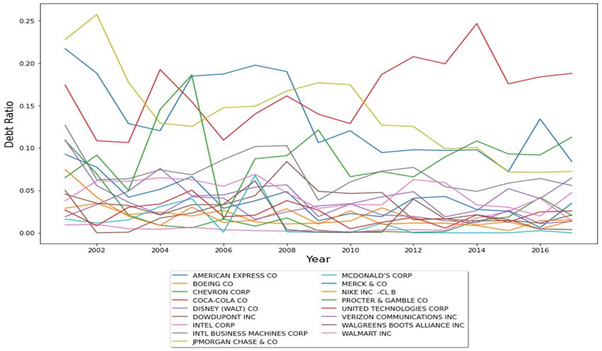
Figures 2 and 3 show plots for the debt ratios of 10 stationary and 15 nonstationary series
companies derived from the KSS PURT with trend and Fourier functions, respectively. Both figures
demonstrate that debt ratios are more volatile in the 15 nonstationary series companies (as seen in
Figure 3) than those of the 10 stationary series companies (as seen in Figure 2).Economies 2020, 8, 76 11 of 19
Table 6. Results of panel KSS test with both trend and Fourier functions.
Sequence OU Statistic Min. KSS Fourier (K) Series
1 −3.0469 (0.0000) −3.8103 2 VERIZON COMMUNICATIONS INC.
2 −2.9080 (0.0002) −3.7087 2 TRAVELERS COS INC.
3 −2.5176 (0.0018) −3.5692 2 PROCTER & GAMBLE CO.
4 −2.4212 (0.0026) −3.4705 2 JOHNSON & JOHNSON
5 −2.4163 (0.0038) −3.4109 2 WALGREENS BOOTS ALLIANCE INC.
6 −2.3273 (0.0064) −2.9576 2 CHEVRON CORP
7 −2.2102 (0.0092) −2.9001 2 JPMORGAN CHASE & CO.
8 −2.1989 (0.0098) −2.7664 2 INTL BUSINESS MACHINES CORP.
9 −2.2092 (0.0102) −2.755 2 EXXON MOBIL CORP.
10 −2.0459 (0.0266) −2.4373 2 MCDONALD’S CORP.
11 −1.8590 (0.1128) −2.1723 2 GOLDMAN SACHS GROUP INC.
12 −1.8014 (0.1190) −2.1411 2 UNITED TECHNOLOGIES CORP.
13 −1.7682 (0.1110) −2.1392 2 INTEL CORP.
14 −1.7444 (0.1260) −2.1057 2 COCA-COLA CO.
15 −1.6280 (0.2860) −1.828 2 PFIZER INC.
16 −1.7476 (0.1892) −1.8243 2 MERCK & CO.
17 −1.7021 (0.3084) −1.7788 2 NIKE INC-CLUB
18 −1.4255 (0.5604) −1.7505 2 AMERICAN EXPRESS CO.
19 −1.0974 (0.7500) −1.7238 2 3M CO.
20 −1.0386 (0.8828) −1.6941 2 WALMART INC.
21 −0.7026 (0.9342) −1.3689 2 CATERPILLAR INC
22 −0.3800 (0.9428) −1.1822 2 DOWDUPONT INC
23 0.1372 (0.9512) −0.5161 2 BOEING CO.
24 0.2777 (0.8470) −0.3554 2 HOME DEPOT INC.
25 −1.0739 (0.4550) −0.3529 2 DISNEY (WALT) CO.
Notes: OU statistics are the invariant average KSS ti,NL statistics (Ucar and Omay 2009). Entries in parentheses
stand for the asymptotic p-value. The significance level is 10%. The maximum lag is 8. The asymptotic p-values
were computed by bootstrap simulations using 5000 replications. Fourier (k) was chosen according to the minimum
sum 2020,
Economies square8, of residuals
x FOR PEERfor Fourier function.
REVIEW 11 of 18
KSSpanel-based
Figure 2. KSS
Figure panel-based unit
unit rootroot
testtest (PURT)
(PURT) for trend
for trend and Fourier
and Fourier function
function stationary
stationary series
series companies.
companies.Figure
Economies 2020,2.8, KSS
76 panel-based unit root test (PURT) for trend and Fourier function stationary series
12 of 19
companies.
Figure 3. KSS PURT for trend and Fourier function nonstationary
nonstationary series
series companies.
companies.
These companies were proven by previous researchers to practice target capital structure via
trade-off theory as influenced by firm size (Daskalakis and Psillaki 2008; Lin et al. 2018; and Sani and
Alifiah 2020) and profitability (Abor 2005; Chang et al. 2009; Črnigoj and Mramor 2009; Chadha and
Sharma 2015; and Sani and Alifiah 2020). Similarly, total assets (proxy for firm size), earnings per share
and dividend payout ratio (proxy for profit), and market value (proxy for growth opportunities) can be
used to further study the causality shown in Table 6. Figures 4–9 show plots regarding the average total
assets, the average EPS (Earnings Per Share) basic from operation, EPS basic with extraordinary items,
EPS basic without extraordinary items, dividend payout ratios, and market value of 10 stationary
series firms and 15 nonstationary series firms from 2001 to 2017, respectively. Apart from some
missing data not used in the calculations, the dividend payout ratios from 2009 to 2017 are included in
Figure 8. In Figures 4–9, the total assets, EPS basic from operation, EPS basic with extraordinary items,
EPS basic without extraordinary items, dividend payout ratios, and market value were clearly higher
in the 10 stationary series firms than in the 15 nonstationary series firms. These outcomes propose
firm size, with profitability and growth opportunities influencing capital structure and supporting
trade-off theories.Economies 2020, 8, 76 13 of 19
Figure 4
Economies 2020, 8, x FOR PEER REVIEW 12 of 18
Figure 9
Figure
Figure4.
4. Firm
Firm assets (firmsize).
assets (firm size).
Figure
Figure5.5.EPS
EPS basic fromoperations.
basic from operations.
1Economies 2020, 8, 76 14 of 19
Figure 5. EPS basic from operations.
Figure
Economies 2020, 8, x FOR PEER REVIEW Figure6.6.EPS
EPSbasic
basic with extraordinaryitems.
with extraordinary items. 13 of 18
Figure 7.7.EPS
Figure EPSbasic
basicwithout extraordinaryitems.
without extraordinary items.Figure 4
Economies 2020, 8, 76 15 of 19
Figure 7. EPS basic without extraordinary items.
Figure 9 Figure 8.
Figure 8. Dividend payout ratios.
Figure 9. Market value.
3.2. Discussion of the Results
In particular, the SPSM process using the KSS PURT with the trend and Fourier functions offers
robust proof showing the debt-ratio stationarity for 10 of 15 firms. These results are consistent with
supporting trade-off theory (e.g., Solomon 1963; Shyam-Sunder and Myers 1999; Hovakimian et al.
2001; Ozkan 2001; Sogorb Mira and López-Gracia 2003; Leary and Roberts 2005; Flannery and Rangan
2006; Hackbarth et al. 2007; Chang and Yu 2010; Elsas 1 and Florysiak 2011; Chen et al. 2019; and Dierker
et al. 2019). In particular, the outcomes of this study were consistent with those of Flannery and Rangan
(2006); Elsas and Florysiak (2011); and Ozkan (2001) in developed countries. Flannery and RanganEconomies 2020, 8, 76 16 of 19
(2006) mentioned the existence of the target capital structure and specified 33% and 34% adjustment
rates of target capital structure for Compustat firms and US firms, respectively. Elsas and Florysiak
(2011) show a 26% adjustment rate for all Compustat companies. Ozkan (2001) displayed target capital
structure and indicated a yearly 43% adjustment rate for an unbalanced panel of 390 UK firms from
1984 to 1996. These outcomes were consistent with those of Sani and Alifiah (2020) and Ahsan et al.
(2016) for developing countries. Ahsan et al. (2016) indicated that short-term, long-term, and total
leverage supported trade-off financing behavior, whereas individual firm results did not. Individual
firm results specified that only 16%, 25%, and 12% of firms had short-term and long-term targets
and total target leverage ratio for firms in Pakistan between 1973 and 2010, respectively. Sani and
Alifiah (2020) proposed that Nigerian listed firms apply dynamic adjustment to reach an optimum
leverage ratio.
Furthermore, the causality of debt-ratio stationarity for 10 of the 25 companies showed that the total
assets, EPS basic from operation, EPS basic with extraordinary items, EPS basic without extraordinary
items, dividend payout ratios, and market capitalization (market value) are clearly higher in the
10 stationary series firms than in the 15 nonstationary series firms, because large-market capitalization
(market value) firms frequently receive fame regarding the generation of quality services, as well as
goods, a history of dependable dividend payments, and stable development. Thus, investments in
large-market capitalization stocks are perhaps more conservative than in small-market capitalization
stocks, possibly decreasing the risk as well as the cost of debt finance. These results propose that firm
size, profitability, and growth opportunities influence capital structure, thereby supporting trade-off
theory. These results are consistent with findings of prior studies, which demonstrated that capital
structure supporting trade-off theory is influenced by firm size (Daskalakis and Psillaki 2008; Lin et al.
2018; Nehrebecka and Dzik-Walczak 2018; and Sani and Alifiah 2020) and profitability (Abor 2005;
Chang et al. 2009; Črnigoj and Mramor 2009; Chadha and Sharma 2015; and Sani and Alifiah 2020).
In particular, these outcomes are consistent with those of Sani and Alifiah (2020); Nehrebecka and
Dzik-Walczak (2018); Ahmad and Etudaiye-Muhtar (2017); and Ahsan et al. (2016) for developing
countries. Nehrebecka and Dzik-Walczak (2018) showed that the firm size and growth opportunities
positively influenced the debt ratio for Polish listed firms, consistent with trade-off theory. Ahsan et al. (2016)
displayed that profitable firms abide by trade-off financing behavior for Pakistan firms. Ahmad and
Etudaiye-Muhtar (2017) showed that firm size, growth opportunity, and profitability affected the
optimum capital structure of Nigerian firms. Sani and Alifiah (2020) proposed that firm size, return on
assets, and tangibility account for target-leverage achievement of Nigerian listed firms.
Several significant policy implications were brought to light in this study. First, overwhelming
evidence in favor of the I (1) nonstationary hypothesis was found, implying that the debt ratios of
15 out of the 25 DJIA samples do not converge. This suggests that shock economic events that affect
debt ratios are permanent. This outcome implies that, following a large structural variation from an
economic event, the debt ratio would not return to its initial stability for a period of time. The fact that
the debt ratio shows I (1) nonstationarity suggests that it should not be possible for the series to predict
future debt ratio movement based on past behavior. Therefore, policymakers ought to look for more
valid methods to attain optimum capital structure for financial system stability.
4. Conclusions
The 30-stock DJIA index is considered to serve as not only a proxy for the health of the wider
US economy, but also represents one of the most cited financial barometers in the world (Paul 2019).
An optimum capital structure is a crucial factor in the success of facing unanticipated economic events,
with all firms attempting to achieve this structure to maintain financial system stability. To fulfil the
optimum capital structure strategy, firm managers should comprehend the stability of their firms’
capital structure. The goal of this study was to examine whether or not the debt ratio is stationary in
listed firms of the DJIA.Economies 2020, 8, 76 17 of 19
Empirical evidence for trade-off theory is copious but generally does not consider structural
breaks. The SPSM and KSS PURTs with Fourier function were employed in this work to verify the
mean-reverting properties of 25 firms listed on the DJIA between 2001 and 2017. In contrast to PURTs,
which join PURT of all the units in the panel and are incapable of deciding I (0) and I (1) series mixtures,
this SPSM apparently categorizes which and how many series are stationary. To the best of our
knowledge, this study is the first to use the KSS PURT with Fourier function via SPSM to evaluate
debt-ratio convergence for listed firms on the DJIA. We hope that this study effectively fills the current
gap in the literature.
The overall results showed debt-ratio stationarity in 10 of 25 firms, supporting trade-off theory.
Moreover, 10 firms were shown to support trade-off theory influenced by corporation size, profitability,
growth opportunity, and dividend payout ratio. For firm managers, whatever structural change exists
in financial markets, the debt ratio temporarily deviates from the target and ultimately returns to its
target. Therefore, control of the trend path or mean value in the long-term is a critical target for the
managers rather than only a temporary policy in the short-term. The widest stock-leverage measure is
the ratio of total liabilities to total assets in this study, which can be thought of as a proxy for what is kept
for shareholders should liquidation occur. However, this does not offer a good denotation of whether
firm default risk was recent. Total liabilities comprise items such as current, provisional, and reserve
liabilities for unpaid salaries, as well as other liabilities for deferred and accrued income and employee
expenses; this might exaggerate the leverage amount (Rajan and Zingales 1995). This study limitation
may help indicate possible research areas in the future.
Author Contributions: The author conceptualized the idea of this paper, collected and analyzed data, and wrote
the manuscript. All authors have read and agreed to the published version of the manuscript.
Funding: This research received no external funding.
Conflicts of Interest: The authors declare no conflict of interest.
References
Abor, Joshua. 2005. The effect of capital structure on profitability: An empirical analysis of listed firms in Ghana.
Journal of Risk Finance 6: 438–45. [CrossRef]
Ahmad, Rubi, and Oyebola Fatima Etudaiye-Muhtar. 2017. Dynamic model of optimal capital structure: Evidence
from Nigerian listed firms. Global Business Review 18: 590–604. [CrossRef]
Ahsan, Tanveer, Man Wang, and Muhammad Azeem Qureshi. 2016. Mean reverting financial leverage: Theory
and evidence from Pakistan. Applied Economics 48: 379–88. [CrossRef]
Bai, Jushan, and Serena Ng. 2004. A Panic Attack on Unit Roots and Cointegration. Econometrica 72: 1127–77.
[CrossRef]
Banerjee, Saugata, Almas Heshmati, and Clas Wihlborg. 2004. The dynamics of capital structure. Research in
Banking and Finance 4: 275–97.
Becker, Ralf, Walter Enders, and Stan Hurn. 2004. A general test for time dependence in parameters. Journal of
Applied Econometrics 19: 899–906. [CrossRef]
Botta, Marco. 2019. Financing Decisions and Performance of Italian SMEs in the Hotel Industry. Cornell Hospitality
Quarterly 60: 335–54. [CrossRef]
Brealey, Richard A., and Stewart Myers. 2003. Principles of Corporate Finance, 7th ed. Pennsylvania: McGraw
Hill Irwin.
Chadha, Saurabh, and Anil K. Sharma. 2015. Determinants of capital structure: An empirical evaluation from
India. Journal of Advances in Management Research 12: 3–14. [CrossRef]
Chang, Chun, and Xiaoyun Yu. 2010. Informational efficiency and liquidity premium as the determinants of
capital structure. Journal of Financial and Quantitative Analysis 45: 401–40. [CrossRef]
Chang, Chingfu, Alice C. Lee, and Cheng F. Lee. 2009. Determinants of capital structure choice: A structural
equation modeling approach. The Quarterly Review of Economics and Finance 49: 97–213. [CrossRef]
Chen, Zhiyao, Jarrad Harford, and Avraham Kamara. 2019. Operating leverage, profitability, and capital Structure.
Journal of Financial and Quantitative Analysis 54: 369–92. [CrossRef]Economies 2020, 8, 76 18 of 19
Choi, In. 2001. Unit root tests for panel data. Journal of International Money and Finance 20: 249–272. [CrossRef]
Choi, In. 2002. Combination unit root tests for cross-sctionally correlated panels. In The Econometric Theory and
Practice: Frontiers of Analysis and Applied Research. Edited by Peter Charles Bonest Phillips, Dean Corbae,
Steven N. Durlauf and Bruce E. Hansen. Cambridge: Cambridge University Press, pp. 311–33. [CrossRef]
Chortareas, Georgios, and George Kapetanios. 2009. Getting PPP right: Identifying mean-reverting real exchange
rates in panels. Journal of Banking and Finance 33: 390–404. [CrossRef]
Christopher, Green, and Guanqun Tong. 2005. Pecking order or trade-off hypothesis? Evidence on the capital
structure of Chinese companies. Applied Economics 37: 2179–89. [CrossRef]
Črnigoj, Matjaž, and Dušan Mramor. 2009. Determinants of capital structure in emerging European economies:
Evidence from Slovenian firms. Emerging Markets Finance & Trade 45: 72–89. [CrossRef]
Daskalakis, Nikolaos, and Maria Psillaki. 2008. Do country or firm factors explain capital structure? Evidence
from SMEs in France and Greece. Applied Financial Economics 18: 87–97. [CrossRef]
DeAngelo, Harry, and Richard Roll. 2015. How stable are corporate capital structures? The Journal of Finance 70:
373–418. [CrossRef]
Dierker, Martin, Inmoo Lee, and Sung Won Seo. 2019. Risk changes and external financing activities: Tests of the
dynamic trade-off theory of capital structure. Journal of Empirical Finance 52: 178–200. [CrossRef]
Elsas, Ralf, and David Florysiak. 2011. Heterogeneity in the speed of adjustment toward target leverage.
International Review of Finance 11: 181–211. [CrossRef]
Enders, Walter, and Junsoo Lee. 2009. The Flexible Fourier Form and Testing for Unit Roots: An Example of the
Term Structure of Interest Rates. Working Paper. Tuscaloosa: Department of Economics, Finance & Legal
Studies, University of Alabama. Available online: http://cba.ua.edu/~{}wenders2/wp-content/uploads/2009/
11/enders_lee_april_29_20091.pdf (accessed on 22 August 2020).
Enders, Walter, and Junsoo Lee. 2012. A unit roots test using a Fourier series to approximate smooth Breaks.
Oxford Bulletin of Economics and Statistics 74: 574–99. [CrossRef]
Fama, Eugene F., and Kenneth R. French. 2002. Testing trade-off and pecking order predictions about dividends
and debt. Review of Financial Studies 15: 1–3. [CrossRef]
Flannery, Mark, and Kasturi P. Rangan. 2006. Partial adjustment toward target capital structures. Journal of
Financial Economics 79: 469–506. [CrossRef]
Frank, Murray Z., and Vidhan K. Goyal. 2009. Capital structure decisions: Which factors are reliably important?
Financial Management 38: 1–37. [CrossRef]
Gallant, Ronald. 1981. On the basis in flexible functional form and an essentially unbiased form: The flexible
Fourier form. Journal of Econometrics 15: 211–353. [CrossRef]
Hackbarth, Dirk, Christopher Hennessy, and Hayne Leland. 2007. Can the tradeoff theory explain debt structure?
Review of Financial Studies 20: 1389–428. [CrossRef]
Hovakimian, Armen, Tim Opler, and Sheridan Titman. 2001. The debt-equity choice. Journal of Financial and
Quantitative Analysis 36: 1–24. [CrossRef]
Im, Kyung So, M. Hashem Pesaran, and Yongcheol Shin. 2003. Testing for unit roots in heterogeneous panels.
Journal of Econometrics 115: 53–74. [CrossRef]
Jarallah, Shaif, Ali. Salman Saleh, and Ruhul Salim. 2019. Examining pecking order versus trade-off theories of
capital structure: New evidence from Japanese firms. International Journal of Finance & Economics 24: 204–11.
[CrossRef]
Ju, Nengjiu, Robert Parrino, Allen M. Poteshman, and Michael S. Weisbach. 2005. Horses and rabbits? Trade-Off
Theory and Optimal Capital Structure. The Journal of Financial and Quantitative Analysis 40: 259–81. [CrossRef]
Kapetanios, George, Andy Snell, and Yongcheol Shin. 2003. Testing for unit root in the nonlinear STAR framework.
Journal of Econometrics 112: 359–79. [CrossRef]
Kwiatkowski, Denis, Peter C. B. Phillips, Peter Schmidt, and Yongcheol Shin. 1992. Testing the null hypothesis of
stationarity against the alternative of a unit root. Journal of Econometrics 54: 159–78. [CrossRef]
Leary, Mark T., and Michael Roberts. 2005. Do firms rebalance their capital structures? Journal of Finance 60:
2575–619. [CrossRef]
Leland, Hayne E. 1994. Corporate debt value, bond covenants, and optimal capital structure. Journal of Finance 49:
1213–52. [CrossRef]
Levin, Andrew, Chien-Fu Lin, and Chia-Shang Chu. 2002. Unit root in panel data: Asymptotic and finite-sample
properties. Journal of Econometrics 108: 1–24. [CrossRef]Economies 2020, 8, 76 19 of 19
Lin, Woon Leong, Nick Yip, Murali Sambasivan, and Jo Ann Ho. 2018. Corporate debt policy of Malaysian SMEs:
Empirical evidence from firm dynamic panel data. Int. Journal of Economics and Management 12: 491–508.
Maddala, Gangadharrao S., and Shaowen Wu. 1999. A comparative study of unit root tests with panel data and a
new simple test. Oxford Bulletin of Economics and Statistics 61: 631–52. [CrossRef]
Miller, Merton H. 1977. Debt and taxes. The Journal of Finance 32: 261–75. [CrossRef]
Modigliani, Franco, and Merton H. Miller. 1958. The cost of capital, corporation finance, and the theory of
investment. American Economic Review 48: 261–97.
Moon, Hyungsik Roger, and Benoit Perron. 2004. Testing for a unit root in panels with dynamic factors. Journal of
Econometrics 122: 81–126. [CrossRef]
Myers, Stewart C. 1984. The capital structure puzzle. Journal of Finance 39: 574–92. [CrossRef]
Myers, Stewart C., and Nicholas S. Majluf. 1984. Corporate financing and investment decisions when firms have
information that investors do not have. Journal of Financial Economics 13: 187–221. [CrossRef]
Nehrebecka, Natalia, and Aneta Dzik-Walczak. 2018. The dynamic model of partial adjustment of the capital
structure: Meta-analysis and a case of Polish enterprises. Zbornik radova Ekonomskog fakulteta u Rijeci/Proceedings
of Rijeka Faculty of Economics 36: 55–81. [CrossRef]
Newey, Whitney K., and Kenneth D. West. 1994. Automatic lag selection in covariance matrix estimation. Review
of Economic Studies 61: 631–653. [CrossRef]
Ozkan, Aydin. 2001. Determinants of capital structure and adjustment to long run target: Evidence from UK
company panel data. Journal of Business Finance & Accounting 28: 175–98. [CrossRef]
Paul, Kosakowski. 2019. Why the Dow Matters. Investopedia. November 14. Available online: https:
//www.investopedia.com/articles/stocks/08/dow-history.asp (accessed on 23 August 2020).
Perron, Pierre. 1989. The great crash, the oil price shock and the unit root hypothesis. Econometrica 57: 1361–401.
[CrossRef]
Pesaran, M. Hashem. 2007. A Simple Panel Unit Root Test in the Presence of Cross Section Dependence. Journal of
Applied Econometrics 22: 265–312. Available online: https://www.jstor.org/stable/25146517 (accessed on 22
August 2020).
Phillips, Peter C. B., and Pierre Perron. 1988. Testing for a unit root in time series regression. Biometrica 75: 335–46.
[CrossRef]
Rajan, Raghran. G., and Luigi Zingales. 1995. What do we know about capital structure? Some evidence from
international data. The Journal of Finance 50: 1421–60. [CrossRef]
Sani, Abdullahi, and Mohd Norfian Alifiah. 2020. Determinants of the capital structure of Nigerian listed firms:
A dynamic panel model. International Journal of Psychosocial Rehabilitation 24: 991–99. [CrossRef]
Shyam-Sunder, Lakshmi, and Stewart C. Myers. 1999. Testing static tradeoff against pecking order models of
capital structure. Journal of Financial Economics 51: 219–44. [CrossRef]
Sogorb Mira, Francisco, and José López-Gracia. 2003. Pecking Order versus Trade-Off: An Empirical Approach
to the Small and Medium Enterprise Capital Structure. Working Paper. Valencia: Instituto Valenciano de
Investigationes Económicas, S.A. [CrossRef]
Solomon, Ezra. 1963. Theory of Financial Management. New York: Columbia University Press. [CrossRef]
Ucar, Nuri, and Tolga Omay. 2009. Testing for unit root in nonlinear heterogeneous panels. Economics Letters 104:
5–8. [CrossRef]
© 2020 by the author. Licensee MDPI, Basel, Switzerland. This article is an open access
article distributed under the terms and conditions of the Creative Commons Attribution
(CC BY) license (http://creativecommons.org/licenses/by/4.0/).You can also read