Detecting Montane Flowering Phenology with CubeSat Imagery - University of Washington
←
→
Page content transcription
If your browser does not render page correctly, please read the page content below
remote sensing
Article
Detecting Montane Flowering Phenology with
CubeSat Imagery
Aji John 1, * , Justin Ong 2 , Elli J. Theobald 1 , Julian D. Olden 3 , Amanda Tan 4 and
Janneke HilleRisLambers 1,5
 1    Department of Biology, University of Washington, Seattle, WA 98195, USA; ellij@uw.edu (E.J.T.);
      jhrl@uw.edu (J.H.)
 2    Paul G. Allen School of Computer Science and Engineering, University of Washington,
      Seattle, WA 98195, USA; cjto2000@uw.edu
 3    School of Aquatic and Fishery Sciences, University of Washington, Seattle, WA 98195, USA; olden@uw.edu
 4    eScience Institute, University of Washington, Seattle, WA 98195, USA; amandach@uw.edu
 5    Institute of Integrative Biology, ETH Zurich, 8092 Zurich, Switzerland
 *    Correspondence: ajijohn@uw.edu

 Received: 31 July 2020; Accepted: 4 September 2020; Published: 7 September 2020

 Abstract: Shifts in wildflower phenology in response to climate change are well documented in the
 scientific literature. The majority of studies have revealed phenological shifts using in-situ observations,
 some aided by citizen science efforts (e.g., National Phenology Network). Such investigations have
 been instrumental in quantifying phenological shifts but are challenged by the fact that limited
 resources often make it difficult to gather observations over large spatial scales and long-time
 frames. However, recent advances in finer scale satellite imagery may provide new opportunities to
 detect changes in phenology. These approaches have documented plot level changes in vegetation
 characteristics and leafing phenology, but it remains unclear whether they can also detect flowering
 in natural environments. Here, we test whether fine-resolution imagery (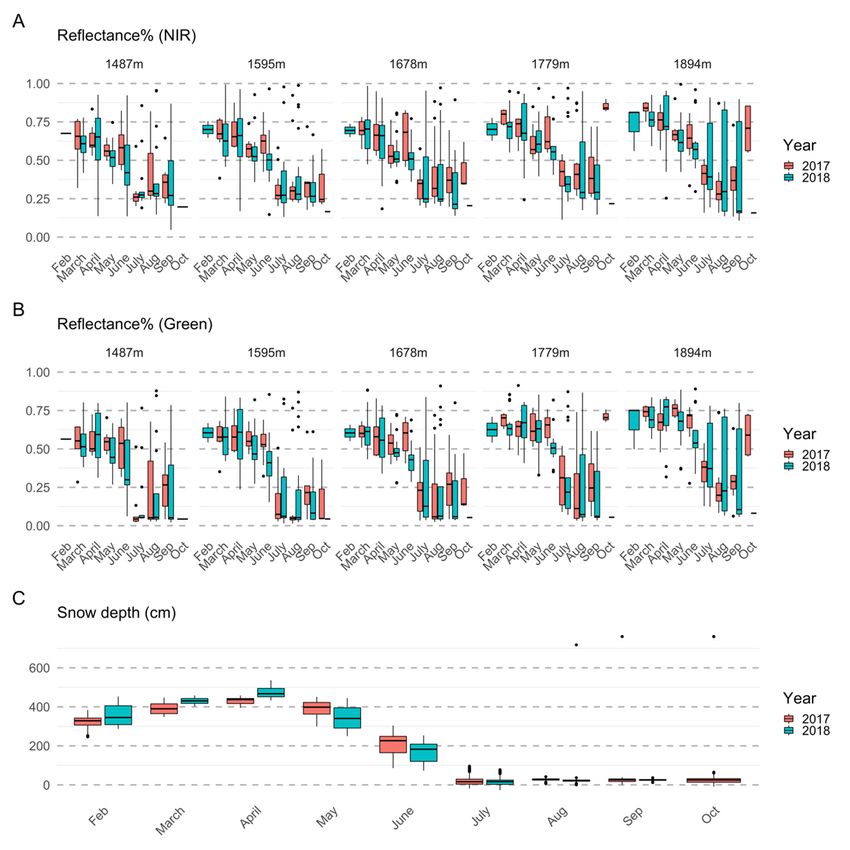
Remote Sens. 2020, 12, 2894                                                                           2 of 22

1. Introduction
      Shifts in seasonal timing of biological events in plants, such as germination, flowering, and fruiting,
in response to climate change have been observed across numerous species [1,2]. For example,
many species demonstrate earlier onset of development and advances in other key life-history events
as the climate warms [3]. Alpine wildflowers are considered good indicators of climatic change, as their
phenology is highly sensitive to spring and summer temperatures and the timing of snowmelt [4].
Such shifts in the timing of flowering of Alpine wildflowers is concerning, as it could disrupt
interactions between Alpine wildflowers and other members of the community, such as pollinators [5].
Understanding and anticipating the impacts of climate change on flowering is therefore paramount to
help inform conservation efforts to ensure the preservation of wildflower meadows in the future [6].
      Mounting evidence from field studies on wildflower phenology compiled by scientists and
volunteer networks document shifts in the timing of flowering [7–9] that seem linked to climate
warming at those locations [10–12]. However, whether it is possible to extrapolate information gained
at smaller spatial scales to larger spatial scales remains uncertain [13]. Quite simply, monitoring
flowering phenology across broader spatial and temporal domains is challenged by limited monetary
and human resources. The ability to detect flowering phenology via remote sensing, if possible,
therefore has the potential to aid in the quantification of fine-scale flowering phenology at large
spatiotemporal scales. Hyperspectral and multispectral imagery has proven to be useful when
analyzing vegetation type and leaf green-up [14] in crop phenological studies [15–17] but, to the best
of our knowledge, has not been used to assess other plant phenological stages in natural systems.
      Recent developments of small satellites, so-called CubeSats, have introduced new possibilities to
monitor land cover at fine spatial and temporal scales. CubeSats have the advantage of high spatial
resolution (in comparison to more traditional satellite imagery) but are limited to few spectral bands
and usually have a small form-factor (dimensions in the order of 10 cm by 10 cm by 30 cm). The low
costs associated with their deployment have resulted in several companies using CubeSat technology
to provide high spatial and temporal coverage of the earth. One such provider is Planet Labs, Inc. [18],
which uses over 150+ (as of 2019) CubeSats to image the entire land surface of the Earth at a daily
time interval and 3–5 m resolution. This imagery provides ecologists with the exciting opportunity to
track a wide array of natural processes that occur at fine spatial scales. Radiometric quality remains an
issue of this data [19]; however, this shortcoming may be improved by cross-calibration using highly
calibrated coarser resolution imagery, like Landsat and Sentinel [20].
      Multispectral bands have long been used to detect plant physiological properties, and CubeSats
offer the possibility of doing so at finer spatial resolutions than other commonly used satellite imagery.
Multispectral products are produced by examining the reflectance spectra that are captured in the
corresponding electromagnetic spectrum and are often used in calculating band ratios [20]. For example,
a commonly used band ratio (or radiometric index) that is used to measure vegetation state is NDVI
(Normalized Difference Vegetation Index—ratio of red and near infrared bands), which has been
found successful when applied to crop type estimation, e.g., in maize, soybean, and wheat, because
of the inherent uniformity in the vegetation [21]. In addition, it has been shown that yellow flowers
can decrease NDVI values in alpine meadows [22], and a cut-off of 0.4 NDVI has been reported as
indicative of full flowering in a study involving sunflower crops [23].
      For this paper, we determined whether multi-spectral imagery obtained from Planet Labs, Inc.,
could help to quantify peak flowering in sub-alpine meadows. We did so by combining satellite
imagery with an existing long-term on-the-ground datasets. The long-term datasets identify the
growing season phenology of wildflower meadows during a period of five years along an elevation
gradient at Mt. Rainier National Park in Washington, USA. We evaluated whether phenological stages
are observable via the spectral bands of PlanetScope (a 3-m, 4-band multispectral image product from
Planet Labs) by using reflectance in the red and near infrared (NIR) bands. Additionally, we evaluated
whether PlanetScope-derived NDVI can be used to delineate flowering. We also combined finer
resolution imagery from Planet with coarser resolution imagery from Sentinel (10 m) and Landsat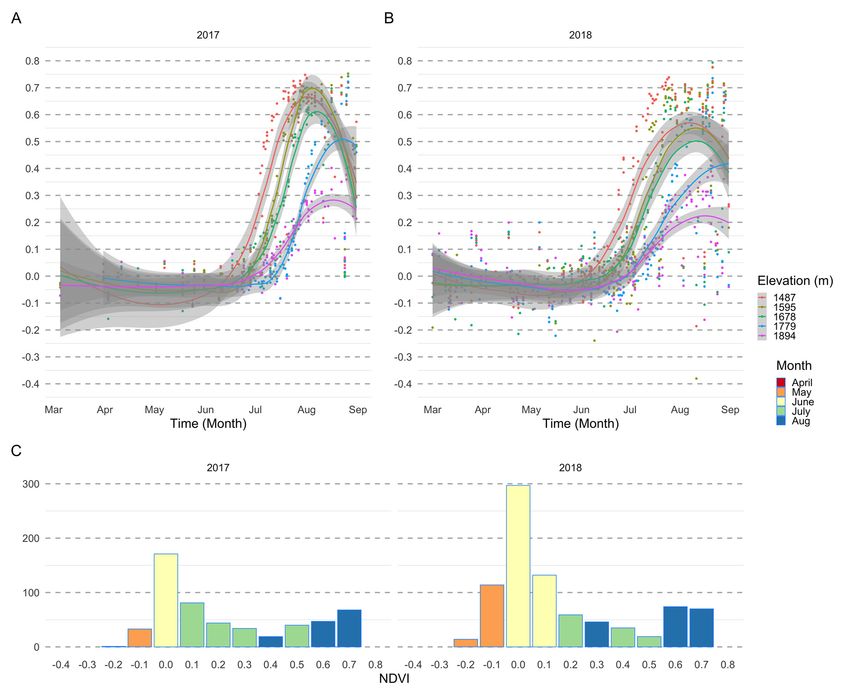
Remote Sens. 2020, 12, 2894                                                                                     3 of 22

  (30 m) to assess whether more accurate phenological detection is possible when combining high these
  two types of imagery. Our objective involved the two following questions. First, can peak flowering
  be detected via either PlanetScope NIR and red bands or a normalized measure, like NDVI? Second,
  is detectability of flowering improved when fine-resolution PlanetScope is combined with coarser
  resolution imagery (with higher quality images), like Landsat and Sentinel?

  2. Materials and Methods

  2.1. Study Site
        Study sites are located in Mt. Rainier National Park (46.8529◦ N, 121.7604◦ W; summit elevation
   4392 m), part of a stratovolcanic mountain range in the Cascade Range of Washington State, USA.
   The regional climate is maritime with dry summers and wet winters. The vegetation is dominated by
   coniferous forests at lower elevations (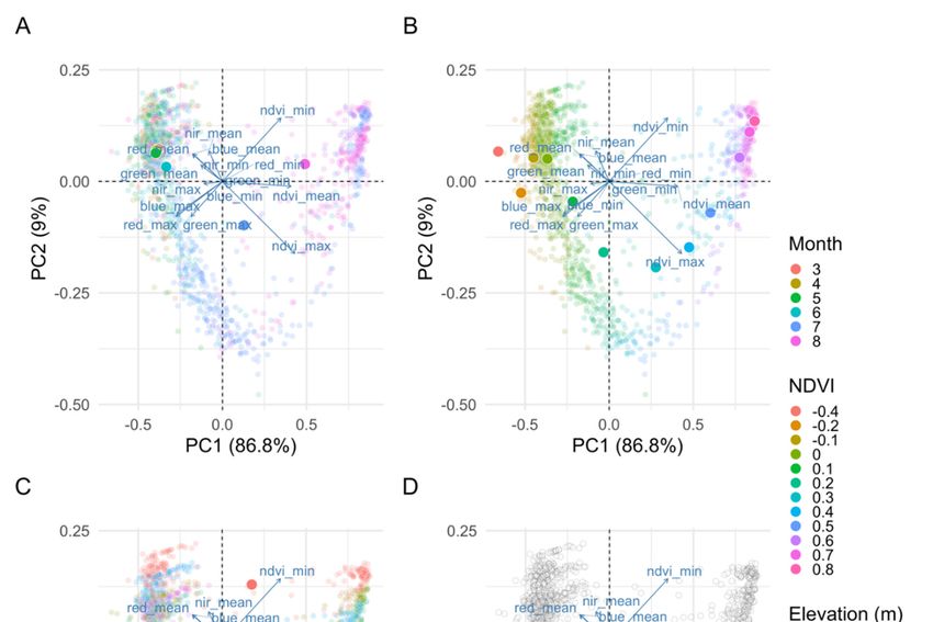
Remote Sens. 2020, 12, 2894                                                                      4 of 22

                               Table 1. Elevation and area of meadow sites.

                              Meadow          Elevation (m)        Area (m2 )
                                1                 1487                 877
                                2                 1595                1328
                                3                 1678                4694
                                4                 1779                1357
                                5                 1894                1136

2.2. Remote Sensing Data
     Remote-sensed imagery were collected from Landsat, Sentinel, and Planet Labs. PlanetScope
imagery from Planet Labs became available only after 2016, so we extracted two years of PlanetScope
imagery (2017–2018), 6 years of imagery from Landsat (2013–2018), and 2 years of imagery from
Sentinel, which was initiated in 2015 (2017–2018). We excluded data from 2016 because of quality
issues with Sentinel imagery (see Appendix D for imagery acquisition and resolution). Thousands
(n = 2893) of images of meadows were analyzed over 5 years of study across providers Landsat 8,
Sentinel-2, and Planet. For all three providers, we extracted summary reflectance values across red,
green, blue, and NIR bands for each meadow area polygon (see Appendix C for band wavelengths).
Additionally, we calculated summary reflectance in short-wave infrared (SWIR) and green chromatic
coordinate (gcc ) for Sentinel imagery for each meadow. We briefly describe the three providers below.
     The Landsat 8 OLI (Operational Land Imager) platform offers 30-m data with high-quality spectral
calibration. The Landsat-8 satellite is one of a series that were launched by the National Aeronautics
and Space Administration (NASA)/U.S. Geological Survey (USGS). Landsat Collection 1 Level-1 data
products are used in the Landsat analysis (here onwards referred as L8).
     Sentinel-2 is owned by the European Space Agency (ESA) and offers 10-m data for red, green,
blue, and NIR bands. Officially called the Copernicus Sentinel-2 mission, Sentinel-2 consists of two
polar-orbiting satellites in the same sun-synchronous orbit, phased at 180 degrees to each other
(Sentinel-2, 2019). Sentinel-2 Level-1B products are used in the Sentinel workflow (here onwards
referred as S2-1B).
     Planet Labs PlanetScope constellation consists of 120+ CubeSats which orbit in two near-polar,
sun-synchronous orbits of ~8◦ and ~98◦ inclination angle at an altitude of roughly 475 km. The CubeSats
acquire both visible (RGB) and NIR data with 12-bit radiometric resolution that images the entire land
surface on Earth daily. Specifically, we used PlanetScope item PSScene4Band (type analytic_sr) in the
Planet workflow (here onwards referred as PS).

2.3. Training and Validation Data: Peak Flowering from on-the Ground Observations
     To associate the satellite images to peak flowering, we developed a method to determine peak
flowering window by elevation: first, we deduced flowering windows from field-based MeadoWatch
observations (collected on the trail adjacent to meadow polygon) observations for 2017 and 2018 when
PS, L8, and S2-1B imagery was available. Then for validation, we determined flowering time for
2013–2015 from observations from MeadoWatch and Theobald et al. (2017) when only L8 imagery
was available. Example kernel density curves of observed flowering of top 10 recorded species for 6
years from MeadoWatch (2013–2018) are presented in Figure 2; 2015 showed a considerable shift in
peak flowering day due to unprecedented warm temperatures (in contiguous United States average
temperature was 2.4 ◦ F above the 20th century average). See Appendix D for imagery and study
period details.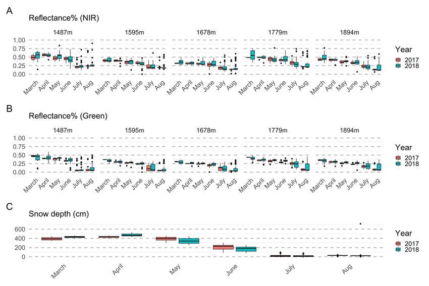
for 2013–2015 from observations from MeadoWatch and Theobald et al. (2017) when only L8 imagery
was available. Example kernel density curves of observed flowering of top 10 recorded species for 6
years from MeadoWatch (2013–2018) are presented in Figure 2; 2015 showed a considerable shift in
peak flowering day due to unprecedented warm temperatures (in contiguous United States average
temperature was 2.4 °F above the 20th century average). See Appendix D for imagery and study
Remote Sens. 2020, 12, 2894                                                                  5 of 22
period details.

     Figure 2.
     Figure   2. In-situ
                 In-situobserved
                          observedflowering
                                      floweringofof10 10
                                                       of the most
                                                          of the    abundant
                                                                  most          meadow
                                                                         abundant        species
                                                                                     meadow      acrossacross
                                                                                               species  a 6-yeara period
                                                                                                                  6-year
     (2016  shown    for completeness).    The dotted    lines indicate  start of the month. Species  include
     period (2016 shown for completeness). The dotted lines indicate start of the month. Species include        Valeriana
     sitchensis (VASI),
     Valeriana            Polygonum
                 sitchensis  (VASI), bistortoides
                                        Polygonum(POBI),     Pedicularis
                                                     bistortoides  (POBI),bracteosa (PEBR),
                                                                             Pedicularis    Microceris
                                                                                         bracteosa     alpestris
                                                                                                    (PEBR),      (MIAL),
                                                                                                              Microceris
     Lupinus   arcticus  (LUAR),   Ligusticum   grayi  (LIGR),   Erigeron  peregrinus  (ERPE),  Erythronium
     alpestris (MIAL), Lupinus arcticus (LUAR), Ligusticum grayi (LIGR), Erigeron peregrinus (ERPE),          montanum
     (ERMO), Castilleja
     Erythronium           parviflora
                    montanum    (ERMO),(CAPA),  Anemone
                                            Castilleja      occidentalis
                                                       parviflora (CAPA),(ANOC).
                                                                             Anemone occidentalis (ANOC).

      Flowering windows were estimated using flowering observations by the MeadoWatch program
      Flowering windows were estimated using flowering observations by the MeadoWatch program
and those reported in Theobald et al. (2017). In both the cases, observer(s) recorded the species, the date
and those reported in Theobald et al. (2017). In both the cases, observer(s) recorded the species, the
(day of the year) and flowering status (‘yes’ or ‘no’) in multiple plots (plots measured 1 m × 1 m
date (day of the year) and flowering status (‘yes’ or ‘no’) in multiple plots (plots measured 1 m x 1 m
in Theobald et al. 2017 and were estimated at ~2 m × 1 m in MeadoWatch). The main difference
in Theobald et al. 2017 and were estimated at ~2 m × 1 m in MeadoWatch). The main difference
between these datasets is that multiple 1 m × 1 m plots were sampled within one of five meadows
between these datasets is that multiple 1 m × 1 m plots were sampled within one of five meadows
sites by Theobald et al. (2017), whereas sampling occurred at nine single MeadoWatch plots, along a
prominent hiking trail. MeadoWatch plots were close to the five Theobald sites, and spanned the
same elevation gradient. Plots within the Theobald et al. (2017) sites were combined to delineate
an area (purple polygons in Figure 1) to fetch the satellite imagery. For the purposes of this study,
the MeadoWatch plots were grouped by elevation using the shortest distance to nearby Theobald site
(Figure 1). Once grouped by elevation, the observations were then separated by year to calculate mean
and standard deviation (SD) of peak flowering day (Figure 3A). The days in one ±SD of the mean was
considered to be peak flowering window for that year and elevation (Figure 3B). Our determination
of flowering windows assumes that all 10 focal species are found in all plots in all years. This is not
a valid assumption but making it does not bias our conclusions as we are making inference at the
community-level. In other words, we are determining peak flower as the date at which there is the
highest probability of seeing any species in flower and are using the 10 most prominent and abundant
species to make this assessment.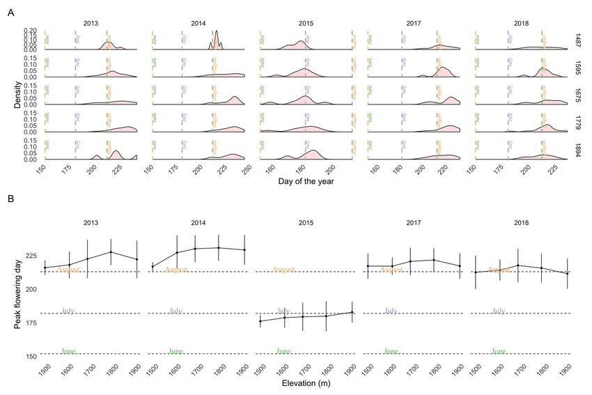
mean was considered to be peak flowering window for that year and elevation (Figure 3B). Our
determination of flowering windows assumes that all 10 focal species are found in all plots in all
years. This is not a valid assumption but making it does not bias our conclusions as we are making
inference at the community-level. In other words, we are determining peak flower as the date at
which there is the highest probability of seeing any species in flower and are using the 10 most
Remote Sens. 2020, 12, 2894                                                                  6 of 22
prominent and abundant species to make this assessment.

     Figure 3. Peak flowering windows using MeadoWatch observations. (A) Kernel density of flowering
     Figure 3. Peak flowering windows using MeadoWatch observations. (A) Kernel density of flowering
     observations by elevation (in meters) and year. (B) Estimated flowering windows calculated using
     observations by elevation (in meters) and year. (B) Estimated flowering windows calculated using
     mean flowering day and ±1 SD; error bars indicate length of the flowering window with the dot
     mean flowering day and ±1 SD; error bars indicate length of the flowering window with the dot
     signifying mean peak flowering day. Note the shift in flowering phenology in 2015, a historically
     signifying mean peak flowering day. Note the shift in flowering phenology in 2015, a historically
     warm year.
     warm year.
2.4. Satellite Data Processing
2.4. Satellite Data Processing
      All processing of satellite imagery data was performed using SWEEP [24], a workflow management
      All processing
platform                of satellite
           for distributed   executionimagery
                                        in clouddata was performed
                                                 infrastructures.  SWEEPusing  SWEEP for
                                                                            workflows [24],acquiring
                                                                                             a workflow
                                                                                                     and
analyzing imagery were developed for PS, L8, and S2-1B and are briefly outlined in the Appendix for
management      platform   for  distributed  execution in cloud   infrastructures. SWEEP workflows    B.
acquiring and analyzing imagery were developed for PS, L8, and S2-1B and are briefly outlined in
the Appendix
2.5. Analysis B.

2.5.1. Importance of Spectral Bands in Flowering
2.5. Analysis
     To assess the relevance of the NIR and red spectral bands to flowering phenology, we employed
2.5.1. Importance of Spectral Bands in Flowering
Principal Component Analysis (PCA) to summarize dominant patterns of variation in the spectral band
data and relate it back to flowering phenology. PCA, a multivariate ordination approach, is a preferable
way to account for correlations among spectral bands [25,26]. We hypothesized that a shift in reflectance
signature in NIR and red bands would be observed in known flowering months and would differ
from the signature when meadows green-up (early summer, after snowmelt) or when the meadows
are covered in snow (early summer and spring). Therefore, for each satellite image we extracted the
minimum, maximum and average pixel value by spectral band for each meadow. We created a spectral
matrix where rows (or objects) corresponded to satellite images (from PS), and columns (descriptors)
included summary measures (minimum, maximum, and mean) of all the bands and NDVI (calculated
using the corresponding red and NIR band). PCA was conducted using PS imagery only because a fine
resolution of 3 m has more spectral representation for an average meadow (typically 30 m by 30 m) and
is more likely to capture the spectral variability in a meadow, i.e., 9-pixel values for an average meadow.
We used PCA in part because it could potentially help identify the reflectance bands that are related to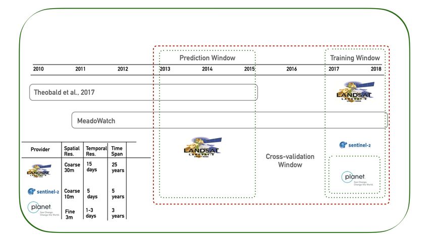
Remote Sens. 2020, 12, 2894 7 of 22
months when flowering is typically observed. Hence, we characterized the relationship between the
flowering meadows and spectral reflectance to understand which band captures flowering.
2.5.2. Flowering Prediction Using Random Forest (RF)
We used a Random Forest (RF) classifier [27] to predict the occurrence of flowering (binary yes or
no) as a function of the spectral variables for years 2013–2015. Random Forest (RF) classifiers are a
model-averaging or ensemble-based approach in which multiple classification tree models are built
using random subsets of the data and predictor variables. This approach uses a recursive partitioning
algorithm to repeatedly partition the data set according to the predictor variables into a nested series
of mutually exclusive groups, each as homogeneous as possible with respect to the response variable.
It requires fewer parameters to be fit, has been shown to be less biased than other machine learning
methods, and is known to be effective in classifying vegetation in remote sensing applications [28,29].
We used Cohen’s kappa statistic to quantify model performance (comparing expected vs. observed
error), and Gini importance to obtain the predictive contributions of the spectral features in the Random
Forest (RF) classifier. We picked the threshold for determining the predicted probability of flowering
by evaluating the receiver operating curve (ROC) and the distribution of true positive rate (sensitivity)
and true negative rate (specificity) with respect to threshold.
We compared how finer resolution imagery compared to the combined resolution imagery by
comparing their Random Forest (RF) performance metrics. We qualitatively assessed peak flowering
using L8 imagery from the years 2013–2015 with two surveys; in-situ observed flowering survey by
Theobald et al., 2017 and MeadoWatch.
All the statistical analyses were performed in R (R Development Core Team 2008).
3. Results
3.1. Importance of Spectral Bands in Flowering
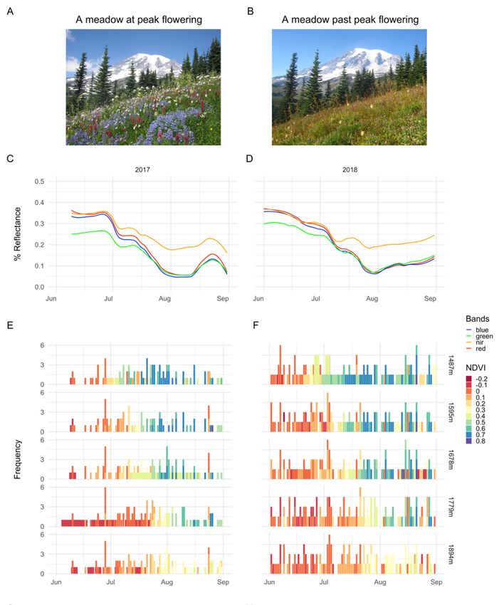
The PS data showed that reflectance in the NIR band is comparatively higher in July and August,
with the other bands showing a high degree of correlation (Figure 4C,D). There is a steady decrease in
reflectance from June to July during snowmelt, and then a rapid decrease in reflectance during July
and August, aligned with the timing of green-up and flowering.
Strong patterns are evident in red and NIR with respect to temporal patterns in observed flowering.
Reflectance in green band is lower when compared to other bands until early July, and then close to
zero reflectance in visible bands (i.e., red, green and blue; also means strong absorption). Increasing
reflectance in the blue band reflects the snowmelt period until early June, followed by months
characterized by decreasing reflectance that indicate greening-up of vegetation. Green-up causes a
steady decrease in reflectance in all bands until an inflection point around late August, evident in 2017
and 2018 (Figure 4C,D). Higher absorbance in visible bands is observed in flowering months except for
NIR, which is correlated with other bands until June, but then shows higher reflectance in flowering
months (Figure 4).
The NDVI profile of the meadow sites by elevation for two years (2017, 2018) show alignment
with flowering months (Figure 4G,H). NDVI is most elevated in late July and August (Figure 4D,E);
coincidently, there is a ramp-up late June followed by a decline in greenness index after August
(Figure A5). NDVI values between −0.1 to +0.1 signifies snow, which is evident in months until June
(Figures A2 and A3). Additionally, NDVI variability is lower at the highest elevation, where vegetation
is sparse, than at the lower elevations; also evident is the lag in peak NDVI by elevation (Figure A4A,B).
We found that average NDVI was linked to flowering months July and August (Figure A4C), also,
NDVI drops after plateauing in late July–early August (PS imagery, Figure A6).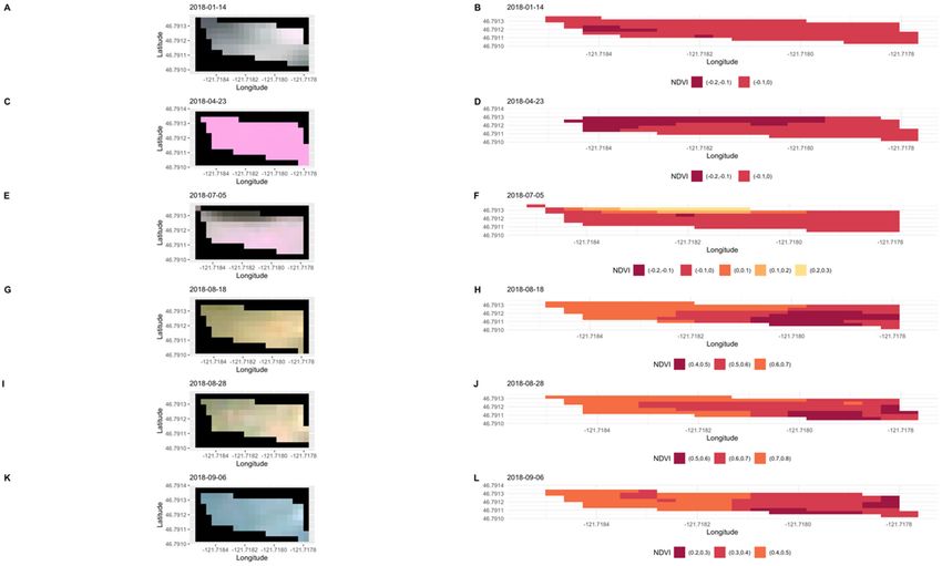
Remote Sens. 2020, 12, 2894                                                                                     8 of 22
   Remote Sens. 2020, 12, x FOR PEER REVIEW                                                                   8 of 24

     Figure 4. (A,B) A typical flowering meadow at peak, and a meadow past the peak flowering. (C,D)
         Figure 4. (A,B)
     Reflectance   profileA of
                            typical   flowering
                                all the  meadowsmeadow
                                                   acrossattwo
                                                            peak,years
                                                                  and a(2017
                                                                         meadow
                                                                             and past theusing
                                                                                  2018)   peak PlanetScope
                                                                                               flowering. (C,D)
                                                                                                             item
         Reflectance  profile  of all  the meadows  across  two  years (2017 and 2018)  using PlanetScope
     PSScene4Band (type analytic_sr) in the Planet workflow (PS). (E,F) Normalized Difference Vegetation   item
         PSScene4Band (type analytic_sr) in the Planet workflow (PS). (E,F) Normalized Difference Vegetation
     Index   (NDVI) profile of all the meadow sites by elevation for two years (2017, 2018) using PS. On the
         Index (NDVI) profile of all the meadow sites by elevation for two years (2017, 2018) using PS. On the
     alternate y-axis is the elevation in meters, and y-axis shows the number of PS captures/meadow having
         alternate y-axis is the elevation in meters, and y-axis shows the number of PS captures/meadow
     the corresponding NDVI threshold. The NDVI thresholds are determined by taking the average of
         having the corresponding NDVI threshold. The NDVI thresholds are determined by taking the
     NDVI metric across the entire meadow. (G,H) Flowering observations for years 2017 and 2018 from
     MeadoWatch; showing dominant 10 flowering species.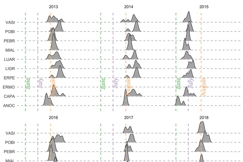
Remote Sens. 2020, 12, 2894                                                                                9 of 22

      A large proportion of the variability in the spectral bands of PS was captured by the first two
principal components (PCs) (Figure 5A,B). In peak flowering months (July and August), PC1 was
positively correlated to mean NDVI, and negatively correlated to mean NIR reflectance values
(Figure 5). Additionally, in peak flowering months, the reflectance in visible and NIR bands are
negatively correlated to PC1. In non-flowering months, PC1 is positively correlated to reflectance
in visible and NIR bands. Seasonal trends are evident, as snow starts declining in the meadows in
May and continues with vegetative growth towards late June and flowering peaking around August.
In typical flowering months July and August, NDVI values are strongly clustered with correspondingly
higher positive mean values of NDVI in the range between 0.6 and 0.8 (Figure 5A,B). Spatial variability
of flowering across elevations is also evident with lower elevations strongly tied to increased NDVI
 Remote
than    Sens. 2020,
      higher        12, x FOR(Figure
               elevations     PEER REVIEW
                                     5C).                                                        10 of 24

      Figure 5. Biplot ordination from the principal component analysis (PCA) for 2 years (2017 and 2018) of
       Figure 5. Biplot ordination from the principal component analysis (PCA) for 2 years (2017 and 2018)
      spectral data from PS for the 5 meadow sites. (A–C) PC1 and PC2, overlain with the centroid (filled
       of spectral data from PS for the 5 meadow sites. (A–C) PC1 and PC2, overlain with the centroid (filled
      large dots) and average summary reflectance’s captured in visible and near infrared (NIR) bands
       large dots) and average summary reflectance’s captured in visible and near infrared (NIR) bands
      colored by month, NDVI, and elevation (blurry dots); (D) the ordination without any highlighting of
       colored by month, NDVI, and elevation (blurry dots); (D) the ordination without any highlighting of
      the individual summary reflectance’s. (A) Seasonal trends are evident; snowmelt in the meadows to
       the individual summary reflectance’s. (A) Seasonal trends are evident; snowmelt in the meadows to
      flowering from upper left to upper right in the panel; blurry dots are colored by month. (B) Flowering
       flowering from upper left to upper right in the panel; blurry dots are colored by month. (B) Flowering
      months (late July and August) demonstrate higher positive mean values of NDVI in panel; blurry dots
       months (late July and August) demonstrate higher positive mean values of NDVI in panel; blurry
      are colored by NDVI. (C) Flowering at sites showing the spread by elevation explained by increase
       dots are colored by NDVI. (C) Flowering at sites showing the spread by elevation explained by
      in NDVI in the flowering months; blurry dots are colored by elevation of the meadow. (D) Strong
       increase in NDVI in the flowering months; blurry dots are colored by elevation of the meadow. (D)
      correlation between visible bands, and NDVI metric that is orthogonal to NIR/visible bands.
       Strong correlation between visible bands, and NDVI metric that is orthogonal to NIR/visible bands.

 3.2. Flowering Predictions Using Random Forest (RF)
     Random Forest (RF) was trained to estimate the flowering window from PS and PS combined
 with coarser resolution satellite imagery. The results showed that the accuracy, i.e., correct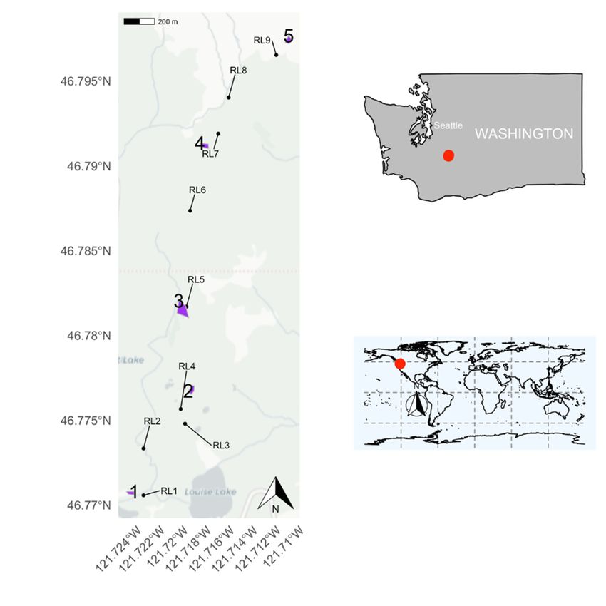
Remote Sens. 2020, 12, 2894                                                                                           10 of 22

3.2. Flowering Predictions Using Random Forest (RF)
     Random Forest (RF) was trained to estimate the flowering window from PS and PS combined
with coarser resolution satellite imagery. The results showed that the accuracy, i.e., correct classification
rate when only PS was used was 70% (Kappa 0.25), when combined with coarser providers was
77% (Kappa 0.39). However, when only coarser imagery was used, accuracy was 72% (Kappa 0.37).
PS explained the most variation at 55% and combined imagery without PS was the lowest with 29%
(Table 2). We used a threshold of 0.25 to determine the predicted probability of flowering.

      Table 2. Metrics when different types of imagery was used. Model combining the PS imagery with
Remote Sens. 2020, 12, x FOR PEER REVIEW                                                           11 of 24
      coarser providers yielded better results than PS only-based model.

                       Metrics
                         Metrics                             PS + PS + L8
                                                                  L8 +    + S2-1BL8 + S2-1B
                                                                       S2-1B            L8 + S2-1B
                                                                                                 PS             PS
                    Accuracy    (%)
                       Accuracy (%)                                  77
                                                                            77             72
                                                                                                    72 70       70
                 Median  CVCVRMSE
                    Median
                              1  1 RMSE                             0.29   0.29           0.27     0.27 0.31   0.31
               Median CVCV
                 Median     1 Variation
                         1 Variation  (%)
                                        (%)                          50     50             29       29 55       55
                          Kappa
                       Kappa                                        0.39   0.39           0.37     0.37 0.25   0.25
                              1   991 cross-validations
                                       99 cross-validationswith
                                                            with 0.10
                                                                 0.10 proportion
                                                                      proportionwithheld
                                                                                 withheldat each run.run.
                                                                                            at each

     In our Random Forest (RF) variable importance analysis, NIR was less relevant than NDVI for
identifying peak flowering.
                  flowering. Mean values of reflectance in NDVI were most important in the RF model
when only fine resolution imagery was used (Figure 6A), whereas,
                                                             whereas, when
                                                                        when using
                                                                               using combined
                                                                                     combined imagery,
                                                                                                 imagery,
the blue band was most important (Figure 6B). However,     NIR is integrated
                                                  However, NIR integrated     into NDVI  as part  of being
a normalized
  normalized measure
               measurewith
                         withthe
                               thered
                                    red  band,
                                       band,   and
                                             and   NDVI
                                                 NDVI    does
                                                      does    stand
                                                           stand  out out in both
                                                                      in both      the datasets,
                                                                              the datasets,      but does
                                                                                            but NIR   NIR
does  not stand
not stand  out asout as much
                  much  as theasred
                                  theband.
                                      red band.

      Figure 6.
      Figure    Relative importance
             6. Relative  importance of
                                      of predictor
                                         predictor spectral
                                                     spectral variables
                                                              variables related
                                                                        related to
                                                                                to flowering
                                                                                   flowering when
                                                                                              when fine
                                                                                                    fine resolution
                                                                                                         resolution
      imagery was
      imagery   was used
                    used versus
                           versus when
                                  when fine-level
                                          fine-level imagery
                                                      imagery was
                                                                was combined
                                                                     combined with
                                                                                 with coarser
                                                                                      coarser resolution
                                                                                               resolution imagery.
                                                                                                           imagery.
      (A) Using  PS only  highlights NDVI    as the top contributor.  (B) PS, along  with L8 and  S2-1B, highlights
      (A) Using PS only highlights NDVI as the top contributor. (B) PS, along with L8 and S2-1B, highlights
      the blue
      the blue band
               band as
                     as the
                        the top
                            top contributor.
                                contributor.

     Predicted peak phenology windows from spectral images aligned with observed phenology in
     Predicted peak phenology windows from spectral images aligned with observed phenology in
some years than the others. The RF model captures the middle (or median) of the flowering window
some years than the others. The RF model captures the middle (or median) of the flowering window
when compared to in-situ but tends to be longer, and the predicted window does not align in most
when compared to in-situ but tends to be longer, and the predicted window does not align in most
cases when compared to MeadoWatch (Figure 7A,B). In comparison with both in-situ and MeadoWatch
cases when compared to MeadoWatch (Figure 7A,B). In comparison with both in-situ and
observations, there is over- and underestimation, which is evident in misaligned start of peak flowering
MeadoWatch observations, there is over- and underestimation, which is evident in misaligned start
of peak flowering window in certain years/elevations and overlapping intervals in some
years/elevations. For 2015, an exceptionally warm year, both Random Forest (RF) models predict with
less overlap but exhibit longer flowering windows that show delayed onset of flowering. Both the
models overpredict the start of the flowering in average years (2013 and 2014) than in a warm year
(2015). The predicted flowering windows aligned better when combined imagery was used than
Remote Sens. 2020, 12, 2894 11 of 22
window in certain years/elevations and overlapping intervals in some years/elevations. For 2015,
an exceptionally warm year, both Random Forest (RF) models predict with less overlap but exhibit
longer flowering windows that show delayed onset of flowering. Both the models overpredict the start
of the flowering in average years (2013 and 2014) than in a warm year (2015). The predicted flowering
Remote Sens. 2020, 12, x FOR PEER REVIEW
windows aligned better when combined imagery was used than when only the finer imagery was12used.of 24
Figure 7. Qualitative comparison of observed window from the in-situ observations of (Theobald
Figure 7. Qualitative comparison of observed window from the in-situ observations of (Theobald et
et al., 2017), MeadoWatch program, and Random Forest (RF) based flowering window. (A) Predicted
al., 2017), MeadoWatch program, and Random Forest (RF) based flowering window. (A) Predicted
and Observed peak flowering window when only 3-m (PS) resolution data was used for training.
and Observed peak flowering window when only 3-m (PS) resolution data was used for training. (B)
(B) Predicted and Observed peak flowering window when 3-m (PS) resolution, along with 10-m (S2-1B)
Predicted and Observed peak flowering window when 3-m (PS) resolution, along with 10-m (S2-1B)
and 30-m (L8) data, was used for training.
and 30-m (L8) data, was used for training.
4. Discussion
4. Discussion
Our study demonstrates that the timing of peak flowering in alpine meadows is detectable using
Our studyCubeSat
fine resolution demonstrates thatand
imagery, thethat
timing
the of peak flowering
addition of coarserinresolution
alpine meadows
imageryisalsodetectable using
substantively
fine resolution
improves modelCubeSat
accuracy.imagery,
We also andfoundthat thatthe
NDVIaddition of often
(a metric coarser resolution
used to quantifyimagery also
vegetative
substantively improves
phenology) better modelflowering
predicted accuracy.phenology
We also foundthan that NDVI
did the NIR (a spectral
metric often
band.usedThetoflowering
quantify
vegetative phenology)
window predicted frombetter
our predicted flowering phenology
model overlapped than did window
with the observed the NIR spectral
in manyband. The
site-year
flowering
combinationswindow predicted
but not in others,from our model
suggesting thatoverlapped
accuracy iswith theissue
still an observed
whenwindow in many
using remote site-
sensing
year combinations
imagery but not in
to detect flowering in others,
meadows. suggesting that accuracy
Finally, more years where is still an issue when
fine-resolution usingoverlaps
imagery remote
sensing imagery to detect
with on-the-ground flowering
phenology datainwould
meadows. Finally,
likely have more
allowed yearsforwhere fine-resolution
improved model andimagerymodel
overlaps
assessment,with
as on-the-ground
we only had 2 yearsphenology data would
of PS imagery likelytohave
to relate allowed for improved
our MeadoWatch model and
observations.
model Weassessment,
found thatas we only
higher had 2 years
reflectance was of PS imagery
observed in NIRto relate
and red to bands
our MeadoWatch
when floweringobservations.
occurred
We found
and can that higher
potentially reflectance
be combined withwas observedcaptured
reflectance in NIR and red bands
in other bandswhen floweringflowering
for improved occurred
and can potentially
detection. be combined
Meadow sites with reflectance
exhibited visibly capturedinin
higher reflectance theother
NIR bands for improved
when flowering flowering
as compared to
detection. Meadow an
meadow green-up, sites exhibited
expected visibly
result higher decrease
as flowers reflectance in the NIR
absorption when
after theflowering as compared
initial green-up [15,30].
to meadow
Strong green-up,
absorbance was an
alsoexpected
found inresult
red and as green
flowers decrease
bands during absorption
flowering,after theequal
as well initialabsorbance
green-up
[15,30]. Strong absorbance was also found in red and green bands during flowering, as well equal
absorbance in the blue band when comparing to NIR. The blue band is typically associated with
green-up time; it is a likely indicator of plant photosystems being active as allocation to vegetative
growth is needed to support the energy required to produce flowers [31]. We found that NIR was
correlated to flowering as is NDVI (which is a function of NIR). We also explored other indices, likeRemote Sens. 2020, 12, 2894 12 of 22
in the blue band when comparing to NIR. The blue band is typically associated with green-up time;
it is a likely indicator of plant photosystems being active as allocation to vegetative growth is needed to
support the energy required to produce flowers [31]. We found that NIR was correlated to flowering as
is NDVI (which is a function of NIR). We also explored other indices, like green chromatic coordinate
(gcc ) index, which is a proxy for greenness that has been found to be useful for detecting flowering other
studies [32]. Our findings suggest that there is a decrease in greenness (i.e., gcc ) past peak green-up
prior to flowering (Figure A5).
Use of visible and NIR bands are instrumental in phenological explorations but might be better
when coupled with additional bands. We show that using visible bands (red, green, and blue) and NIR
bands were sufficient in narrowing down the flowering window, but use of finer bands at the red-edge
region might help further augment the flowering signal [33,34]. For example, use of SWIR has been
found to be useful in accentuating signals of senescent vegetation. In addition, a recent announcement
by Planet to provide additional bands (between 5 to 8) on next generation CubeSats could improve the
phenological assessment at finer resolutions.
NDVI was found to be a significant predictor of peak flowering phenology in alpine/subalpine
meadows. NDVI normalizes NIR and red bands and has been shown to be associated with green-up [35].
Furthermore, flowering must be preceded by peak green-up, which is evident by plateauing of NDVI
(Figure A4A,B), signifying saturation because of chlorophyll accumulation [36]. Although reflectance
in NIR visually shows the strongest pattern during peak flowering (Figure 4C,D), we actually found
that a normalized measure like NDVI (which incorporates NIR) better predicts flowering (Figure 6A,B).
The NDVI-based metric is usually applied in crop classification studies [37], but we also found it useful
for detecting flowering in alpine meadows—an important result as it indicates this metric may also be
applicable in studies which are looking to differentiate other phenological stages.
Despite the fact that NDVI was a reliable metric in our study, we recognize that it also has a
number of shortcomings. Remotely sensed NDVI has been acknowledged as differing from true NDVI
because of atmospheric effects and varying soil brightness, both of which can differ from image to
image [38]. Although soil blotches are not common in alpine meadows except at very high elevations,
the largest challenge is associated with canopy background limitations [39]. For this reason, Enhanced
Vegetation Index (EVI) is often used as an alternative to NDVI to address the soil and atmospheric
limitations [16]. We therefore suggest that EVI and the other related indices should be explored for
their utility in predicting phenological stages beyond vegetative ones, including the combination of
several indices to improve measurement accuracy.
We show that combining several types of satellite imagery leads to enhanced predictions of
flowering phenology. Specifically, by combining 3-m spectral imagery with 10-m and 30-m imagery,
our model predictions showed better overlap with observed flowering windows when compared to
just the finer resolution model. However, the combined model tended to overpredict the start of the
flowering windows (except in the anomalously warm year—2015). Similar studies have shown that
multi-resolution data analysis improves results: “fuzzier” low resolution data can provide “big picture”
information, and, when combined with the lower-resolution data, finer details can be revealed [40].
Our results also suggest that coarser 30-m Landsat imagery can be useful to infer peak flowering.
The model parameterized with combined imagery (including finer scale Planet imagery) was able to
infer peak flowering when applied to Landsat in years where only coarser scale imagery was available.
Additional improvements to model predictions are possible by refining atmospheric corrections used
for Landsat and Sentinel; in this study, we uniformly applied corrections across each individual band
in order to account for atmospheric absorption, such as the effect of haze (Appendix A). However,
these effects are not likely to be uniform. Future work should examine the effect of band-specific
atmospheric corrections on phenology prediction accuracy.
Despite having an amalgam of satellite imagery of the meadows, one fundamental question is that
are we able to distinguish the flowering signal from the background, i.e., soil, rocks or green vegetative
growth [41,42]. PS comes with only 4 bands and has overlapping bands that might lead to pixel qualityRemote Sens. 2020, 12, 2894 13 of 22 issues [43,44], and other coarser providers have constraints of resolution and frequency of captures. However, meadow wildflower phenology progresses seasonally in a predictable manner. In the springtime, plants are covered with snow; when snow melts, they green-up, and then peak-flowering happens, and then snow falls again, covering all vegetation. This cycle culminates in about 4 months. We see this same 4-month cycle in the satellite signal through RGB composite and NDVI (Figure A6). Our method is bound by these constraints, but having more on-the-ground observations in time and even better satellite resolution (e.g.,
Remote Sens. 2020, 12, 2894                                                                          14 of 22

values measured by the sensors and have no meaningful value. TOA is converted to BOA because
BOA takes into account atmospheric effects, such as cloud cover, aerosol gases, etc. For Landsat,
the equation for DN to TOA conversion is

                                                 Mρ Qcal + Aρ
                                          ρλ =                  .                                      (A1)
                                                   cos(θSZ )

     In Equation (A1), ρλ = TOA planetary reflectance, Mρ = band-specific multiplicative rescaling
factor, Aρ = band-specific additive rescaling factor, Qcal = quantized and calibrated DN pixel value,
and θSZ = solar zenith angle for solar correction.
     Mρ is 2 × 10⁻⁵ , and Aρ is −0.1, which are both provided in the metadata file. The solar elevation
(θSE = 90 − θSZ ) angle is provided in the metadata file as an average of the entire tile, but Landsat
provides a tool to get the θSZ for each pixel in a specific band. This is used instead of the approximation.
     Once TOA reflectance is calculated, a scatter value is subtracted in order to get BOA reflectance.
TOA is only reflecting from above the atmosphere. This scatter value is calculated by using a method
called Frequency 50 Minus 0.008 (F50 0.8%) developed by GIS Ag Maps [48]. This is an image-based
atmospheric correction model based on the Chavez Landsat TM histogram method [49]. This model
only accounts for atmospheric scattering and assumes a constant haze value throughout the entire
image. This constant haze value is determined by a relative scatter lookup table provided by GIS Ag
Maps. This is by no means the most accurate way to derive surface reflectance as it is an image-based
correction algorithm; however, it was used here because of its accuracy and simplicity.

Appendix B
    Workflows for acquiring and analyzing Landsat, Sentinel, and Planet satellite images were written
and executed on SWEEP [24], a scalable workflow management platform.

Appendix B.1. Landsat
      The workflow begins with setting the input boundaries of the meadow sites, which are subsequently
run against the USGS Earthdata Explorer API (EE API), along with the date ranges to fetch the available
scenes. Scenes are available on EE API and AWS S3 (a cloud data storage product) as part of its
open data program. EE API provides functionality to search and download Landsat imagery for free.
The workflow was designed from the ground-up and is made available to ensure reproducibility.
We chose to use both of these services to overcome an EE API limit on parallel downloads. Once a
set of scenes is returned by EE API, the list of scenes was checked against AWS S3 for availability.
Once matched scenes are found, they are downloaded from S3 and then re-projected (projection WGS
84 is used for this workflow), cropped, and radio-metrically corrected using the Landsat TM histogram
method by (Chavez Jr, 1988). Next, statistical measures (min, max, and mean) are calculated across
all the bands in visible and NIR spectra at the meadow level. Finally, the results are written to a
comma-separated values (CSV) file which includes the statistical values for each band, the name of the
feature (meadow site), and the date.

Appendix B.2. Sentinel
     The workflow starts by setting a list of polygons referring to meadow sites. Next, the workflow
gets the applicable AWS scenes using the sentinelhub Python package with a spatial and temporal filter.
The results include the AWS S3 URL, as well as the date of each of the scenes, which are both extracted
for all of the available scenes. Once the scenes are found for each meadow, retrieving and refining of
the data for each scene is subsequently run in parallel. This includes fetching, re-projecting, cropping,
and refining the image data. Re-projecting and cropping are similar to the Landsat implementation
mentioned above.
Remote Sens. 2020, 12, 2894 15 of 22
The image data conversion for this workflow is less computationally demanding than that of
the Landsat workflow because Sentinel-2 L1C data comes as Top-of-Atmosphere (TOA) reflectance.
Thus, we only needed to subtract each band’s scatter value to reach Bottom-of-Atmosphere (BOA)
reflectance, also known as surface reflectance. The method used to find the scatter value is the same
one used in the Landsat workflow, except that the Sentinel relative scatter table was used, as opposed
to the Landsat relative scatter table. Both of the tables are provided by GIS Ag Maps [49] to find the
scatter values
Remote Sens. 2020,for
12, the bands.
x FOR PEER REVIEW 16 of 24
Appendix B.3. Planet
Here, all the interactions are made via the the Planet
Planet API
API through
through thethe SWEEP
SWEEP tasks.
tasks. The workflow
starts by using the meadow polygons to search for images within the desired
starts by using the meadow polygons to search for images within the desired date range. date range. TheThe
results are
results
image identifiers
are image that that
identifiers are passed to thetonext
are passed the task, whichwhich
next task, issuesissues
an APIancall
APItocall
activate each image
to activate scene.
each image
The next
scene. task
The sends
next taska clipping request torequest
sends a clipping the API,towhereby
the API,the meadow
whereby theis meadow
clipped from the larger
is clipped scene.
from the
A download request is then sent for each image, which, when ready, is furnished
larger scene. A download request is then sent for each image, which, when ready, is furnished via avia a time-sensitive
link. Finally, the
time-sensitive images
link. are downloaded,
Finally, the images are and metrics calculated
downloaded, for each
and metrics band. The
calculated foroutput is written
each band. The
to a CSV file that has band metrics time-stamped for each meadow.
output is written to a CSV file that has band metrics time-stamped for each meadow.
Appendix
Appendix C
C
Table A1.
Table A1. Wavelengths
Wavelengths (in
(in nanometer,
nanometer, µm)
μm) of
of spectral
spectral bands
bands by
by different
different satellite
satellite imagery
imagery providers.
providers.
Band
Band Landsat
Landsat88 Sentinel-2
Sentinel-2 Planet
Planet
Blue
Blue
0.45–0.51
0.45–0.51
0.45–0.52
0.45–0.52
0.450.45
= 0.51
= 0.51
Green
Green 0.53–0.59
0.53–0.59 0.54–0.57
0.54–0.57 0.50–0.59
0.50–0.59
Red
Red 0.64–0.67
0.64–0.67 0.65–0.68
0.65–0.68 0.59–0.67
0.59–0.67
NIR
NIR 0.85–0.88
0.85–0.88 0.78–0.90
0.78–0.90 0.78–0.86
0.78–0.86
SWIR
SWIR 1.5–1.6
1.5–1.6 0.9–1.7
0.9–1.7 N/AN/A
Appendix D
Figure A1. Time frame of fine resolution data versus coarse resolution data of the study.
Figure A1. Time frame of fine resolution data versus coarse resolution data of the study.Remote Sens. 2020, 12, 2894 16 of 22
Remote Sens. 2020, 12, x FOR PEER REVIEW 17 of 24
Appendix
Appendix EE
Figure A2. Planet reflectance comparison of NIR and green band showing snowmelt followed by
Figure A2. Planet reflectance comparison of NIR and green band showing snowmelt followed by
green-up and flowering. (A) NIR reflectance is higher in snow months than in vegetative and flowering
green-upsignified
months, and flowering. (A)
by positive NIR reflectance
correlation is higher
of reflectance’s withinsnow-depth.
snow months than in
(B) Green vegetative
reflectance and
shows
flowering months, signified by positive correlation of reflectance’s with snow-depth.
lower reflectance (i.e., higher absorption) after the snow-melt, signifying green-up. (C) Snow-depth(B) Green
reflectance
plot shows
from the lower reflectance
metrological (i.e., highersnow-free
records highlighting absorption) after the
months snow-melt,
after June. signifying green-up.
(C) Snow-depth plot from the metrological records highlighting snow-free months after June.Remote Sens. 2020, 12, 2894 17 of 22
Remote Sens. 2020, 12, x FOR PEER REVIEW 18 of 24
Figure A3. Combined Sentinel and Landsat reflectance comparison of NIR and green band showing
Figure A3. Combined Sentinel and Landsat reflectance comparison of NIR and green band showing
snowmelt followed by green-up and flowering. (A) NIR reflectance is higher in snow months than in
snowmelt followed by green-up and flowering. (A) NIR reflectance is higher in snow months than in
vegetative and flowering months, signified by positive correlation of reflectance’s with snow-depth;
vegetative and flowering months, signified by positive correlation of reflectance’s with snow-depth;
however, note the upward trend of NIR in late September and October, signifying onset of snow or
however, note the upward trend of NIR in late September and October, signifying onset of snow or
drying vegetation. (B) Green reflectance shows lower reflectance (i.e., higher absorption) after the
drying vegetation. (B) Green reflectance shows lower reflectance (i.e., higher absorption) after the
snow-melt, signifying green-up. (C) Snow-depth plot from the metrological records highlighting
snow-melt, signifying green-up. (C) Snow-depth plot from the metrological records highlighting
snow-free months after June.
snow-free months after June.Remote Sens. 2020, 12, 2894 18 of 22
Remote Sens. 2020, 12, x FOR PEER REVIEW 19 of 24
Figure A4. NDVI curve (loess smoothing) using Planet reflectance for years 2017–2018, showing the
Figure A4. NDVI curve (loess smoothing) using Planet reflectance for years 2017–2018, showing the
peak green-up around late July and also showing the phase lag by elevation. (A) 2017 NDVI values
peak green-up around late July and also showing the phase lag by elevation. (A) 2017 NDVI values
going from −0.2 to 0.8 capturing snow on the ground to flowering; also, notice the lag in peak NDVI
going from −0.2 to 0.8 capturing snow on the ground to flowering; also, notice the lag in peak NDVI
confirming the snow-melt lag that is driven by elevation. (B) Similar patterns as 2017, 2018 NDVI
confirming the snow-melt lag that is driven by elevation. (B) Similar patterns as 2017, 2018 NDVI
values going from −0.2 to 0.8, capturing snow on the ground to flowering; also, notice the lag in peak
values going from −0.2 to 0.8, capturing snow on the ground to flowering; also, notice the lag in peak
NDVI confirming the snow-melt lag that is driven by elevation. (C) Histogram of NDVI values binned
NDVI confirming the snow-melt lag that is driven by elevation. (C) Histogram of NDVI values binned
by year with the average month that it was observed in shaded.
by year with the average month that it was observed in shaded.Remote Sens. 2020, 12, 2894 19 of 22
Remote Sens. 2020, 12, x FOR PEER REVIEW 20 of 24
A B
Figure A5.Green
FigureA5. GreenChromatic
ChromaticCoordinate
Coordinate(g(gcccc)) that
that isisaaproxy
proxyof ofgreenness
greennesscalculated
calculatedusing
usingSentinel
Sentinel
reflectance
reflectance as data existed after August for years 2017–2018, showing the decline in green-uparound
as data existed after August for years 2017–2018, showing the decline in green-up around
late
lateAugust
Augustbutbutmoderated
moderatedby byelevation.
elevation. (A)
(A)2017,
2017,capturing
capturingthetheramp-up
ramp-upafter
afterlate
lateJune
Juneright
rightafter
after
snow-melt
snow-meltand anddecline
declineafter
afterAugust;
August;highest
highestelevation
elevationsites
siteshave
havevery
veryshort
shortgreen-up.
green-up.(B)(B)Similar
Similar
patterns
patternsasas2017, 2018
2017, shows
2018 ramp-up
shows in greenness
ramp-up in greennessaround late June
around lateand drop
June in drop
and greenness after August.
in greenness after
August.Remote Sens. 2020, 12, 2894 20 of 22
Remote Sens. 2020, 12, x FOR PEER REVIEW 21 of 24
Figure A6.True
FigureA6. Truecolor
colorcomposite
composite(red,
(red,green,
green,andandblue
blueband
bandcombined)
combined)andandcorresponding
correspondingNDVI
NDVIof of
Meadow
Meadow 4 (1779 m) for the year 2018. Column 1 for the panel gives a sense of how the meadowisis
4 (1779 m) for the year 2018. Column 1 for the panel gives a sense of how the meadow
changing
changingduring
duringthe
thewhole
whole year; starting
year; from
starting covered
from with
covered snow
with (A,C,E),
snow thenthen
(A,C,E), meadow green-up
meadow and
green-up
flowering (G,I,K),
and flowering to senescence
(G,I,K), (M,O),(M,O),
to senescence and back
andtoback
covered with snow
to covered with(Q). Column
snow 2 show the
(Q). Column change
2 show the
in seasonality that is captured by NDVI; it shows in months till July NDVI remains below 0.2–0.3
change in seasonality that is captured by NDVI; it shows in months till July NDVI remains below 0.2–
(B,D,F), then a sharp increase in NDVI (H,J,L), and finally back to low levels of NDVI confirming
0.3 (B,D,F), then a sharp increase in NDVI (H,J,L), and finally back to low levels of NDVI confirming
snow (N,P,R).
snow (N,P,R).
References
References
1. Burrows, M.T.; Schoeman, D.S.; Buckley, L.B.; Moore, P.; Poloczanska, E.S.; Brander, K.M.; Brown, C.;
1. Burrows, M.T.; Schoeman, D.S.; Buckley, L.B.; Moore, P.; Poloczanska, E.S.; Brander, K.M.; Brown, C.;
Bruno, J.F.; Duarte, C.M.; Halpern, B.S.; et al. The Pace of Shifting Climate in Marine and Terrestrial
Bruno, J.F.; Duarte, C.M.; Halpern, B.S.; et al. The Pace of Shifting Climate in Marine and Terrestrial
Ecosystems. Science 2011, 334, 652–655. [CrossRef]
Ecosystems. Science 2011, 334, 652–655, doi:10.1126/science.1210288.
2. Parmesan, C. Ecological and Evolutionary Responses to Recent Climate Change. Annu. Rev. Ecol. Evol. Syst.
2. Parmesan, C. Ecological and Evolutionary Responses to Recent Climate Change. Annu. Rev. Ecol. Evol. Syst.
2006, 37, 637–669. [CrossRef]
2006, 37, 637–669, doi:10.1146/annurev.ecolsys.37.091305.110100.
3. Parmesan, C.; Hanley, M.E. Plants and climate change: Complexities and surprises. Ann. Bot. 2015, 116,
3. Parmesan, C.; Hanley, M.E. Plants and climate change: Complexities and surprises. Ann. Bot. 2015, 116,
849–864. [CrossRef] [PubMed]
849–864, doi:10.1093/aob/mcv169.
4. Theobald, E.J.; Breckheimer, I.; HilleRisLambers, J. Climate drives phenological reassembly of a mountain
4. Theobald, E.J.; Breckheimer, I.; HilleRisLambers, J. Climate drives phenological reassembly of a mountain
wildflower meadow community. Ecology 2017, 98, 2799–2812. [CrossRef] [PubMed]
wildflower meadow community. Ecology 2017, 98, 2799–2812, doi:10.1002/ecy.1996.
5. Ogilvie, J.E.; Griffin, S.R.; Gezon, Z.J.; Inouye, B.D.; Underwood, N.; Inouye, D.W.; Irwin, R.E. Interannual
5. Ogilvie, J.E.; Griffin, S.R.; Gezon, Z.J.; Inouye, B.D.; Underwood, N.; Inouye, D.W.; Irwin, R.E. Interannual
bumble bee abundance is driven by indirect climate effects on floral resource phenology. Ecol. Lett. 2017, 20,
bumble bee abundance is driven by indirect climate effects on floral resource phenology. Ecol. Lett. 2017,
1507–1515. [CrossRef]
20, 1507–1515, doi:10.1111/ele.12854.Remote Sens. 2020, 12, 2894 21 of 22
6. Panetta, A.M.; Stanton, M.L.; Harte, J. Climate warming drives local extinction: Evidence from observation
and experimentation. Sci. Adv. 2018, 4, eaaq1819. [CrossRef]
7. Theobald, E.J.; Ettinger, A.K.; Burgess, H.K.; DeBey, L.B.; Schmidt, N.R.; Froehlich, H.E.; Wagner, C.;
HilleRisLambers, J.; Tewksbury, J.; Harsch, M.A.; et al. Global change and local solutions: Tapping the
unrealized potential of citizen science for biodiversity research. Biol. Conserv. 2015, 181, 236–244. [CrossRef]
8. Schwartz, M.D.; Betancourt, J.L.; Weltzin, J.F. From Caprio’s lilacs to the USA National Phenology Network.
Front. Ecol. Environ. 2012, 10, 324–327. [CrossRef]
9. Kudo, G. Dynamics of flowering phenology of alpine plant communities in response to temperature and
snowmelt time: Analysis of a nine-year phenological record collected by citizen volunteers. Environ. Exp. Bot.
2020, 170, 103843. [CrossRef]
10. CaraDonna, P.J.; Iler, A.M.; Inouye, D.W. Shifts in flowering phenology reshape a subalpine plant community.
Proc. Natl. Acad. Sci. USA 2014, 111, 4916–4921. [CrossRef]
11. Dunne, J.A.; Harte, J.; Taylor, K.J. Subalpine meadow flowering phenology responses to climate change:
Integrating experimental and gradient methods. Ecol. Monogr. 2003, 73, 69–86. [CrossRef]
12. Inouye, D.W.; Saavedra, F.; Lee-Yang, W. Environmental influences on the phenology and abundance of
flowering by Androsace septentrionalis (Primulaceae). Am. J. Bot. 2003, 90. [CrossRef] [PubMed]
13. Wolkovich, E.M.; Cook, B.I.; Allen, J.M.; Crimmins, T.M.; Betancourt, J.L.; Travers, S.E.; Pau, S.; Regetz, J.;
Davies, T.J.; Kraft, N.J.B.; et al. Warming experiments underpredict plant phenological responses to climate
change. Nature 2012, 485, 494–497. [CrossRef] [PubMed]
14. Shores, C.R.; Mikle, N.; Graves, T.A. Mapping a keystone shrub species, huckleberry (Vaccinium
membranaceum), using seasonal colour change in the Rocky Mountains. Int. J. Remote Sens. 2019, 40,
5695–5715. [CrossRef]
15. Chen, B.; Jin, Y.; Brown, P. An enhanced bloom index for quantifying floral phenology using multi-scale
remote sensing observations. ISPRS J. Photogramm. Remote Sens. 2019, 156, 108–120. [CrossRef]
16. Fang, S.; Tang, W.; Peng, Y.; Gong, Y.; Dai, C.; Chai, R.; Liu, K. Remote estimation of vegetation fraction and
flower fraction in oilseed rape with unmanned aerial vehicle data. Remote Sens. 2016, 8, 416. [CrossRef]
17. Horton, R.; Cano, E.; Bulanon, D.; Fallahi, E. Peach Flower Monitoring Using Aerial Multispectral Imaging.
J. Imaging 2017, 3, 2. [CrossRef]
18. Planet. Planet Application Program Interface: In Space for Life on Earth; Planet: San Francisco, CA, USA, 2018.
19. Oliphant, A.J.; Thenkabail, P.S.; Teluguntla, P.; Xiong, J.; Gumma, M.K.; Congalton, R.G.; Yadav, K. Mapping
cropland extent of Southeast and Northeast Asia using multi-year time-series Landsat 30-m data using a
random forest classifier on the Google Earth Engine Cloud. Int. J. Appl. Earth Obs. Geoinf. 2019, 81, 110–124.
[CrossRef]
20. Houborg, R.; McCabe, M. Daily Retrieval of NDVI and LAI at 3 m Resolution via the Fusion of CubeSat,
Landsat, and MODIS Data. Remote Sens. 2018, 10, 890. [CrossRef]
21. Bolton, D.K.; Friedl, M.A. Forecasting crop yield using remotely sensed vegetation indices and crop phenology
metrics. Agric. For. Meteorol. 2013, 173, 74–84. [CrossRef]
22. Shen, M.; Chen, J.; Zhu, X.; Tang, Y. Yellow flowers can decrease NDVI and EVI values: Evidence from a field
experiment in an alpine meadow. Can. J. Remote Sens. 2009, 35, 99–106. [CrossRef]
23. Herbei, M.V.; Sala, F. Use landsat image to evaluate vegetation stage in sunflower crops. AgroLife Sci. J. 2015,
4, 79–86.
24. John, A.; Ausmees, K.; Muenzen, K.; Kuhn, C.; Tan, A. SWEEP: Accelerating Scientific Research Through
Scalable Serverless Workflows. In UCC ’19 Companion: Proceedings of the 12th IEEE/ACM International
Conference on Utility and Cloud Computing Companion, Auckland, New Zeland, 2–5 December 2019; ACM Press:
New York, NY, USA, 2019; pp. 43–50.
25. Huete, A.R. Remote sensing for environmental monitoring. In Environmental Monitoring and Characterization;
Elsevier: Cambridge, MA, USA, 2004; pp. 183–206. ISBN 978-0-12-064477-3.
26. Jolliffe, I.T.; Cadima, J. Principal component analysis: A review and recent developments. Phil. Trans. R.
Soc. A 2016, 374, 20150202. [CrossRef] [PubMed]
27. Cutler, D.R.; Edwards, T.C.; Beard, K.H.; Cutler, A.; Hess, K.T.; Gibson, J.; Lawler, J.J. Random Forests for
Classification in Ecology. Ecology 2007, 88, 2783–2792. [CrossRef] [PubMed]
28. Belgiu, M.; Csillik, O. Sentinel-2 cropland mapping using pixel-based and object-based time-weighted
dynamic time warping analysis. Remote Sens. Environ. 2018, 204, 509–523. [CrossRef]You can also read