Derivation and validation of gray box models to estimate noninvasive in vivo percentage glycated hemoglobin using digital volume pulse waveform ...
←
→
Page content transcription
If your browser does not render page correctly, please read the page content below
www.nature.com/scientificreports
OPEN Derivation and validation
of gray‑box models to estimate
noninvasive in‑vivo percentage
glycated hemoglobin using digital
volume pulse waveform
Shifat Hossain, Shantanu Sen Gupta, Tae‑Ho Kwon & Ki‑Doo Kim*
Glycated hemoglobin and blood oxygenation are the two most important factors for monitoring
a patient’s average blood glucose and blood oxygen levels. Digital volume pulse acquisition is a
convenient method, even for a person with no previous training or experience, can be utilized to
estimate the two abovementioned physiological parameters. The physiological basis assumptions
are utilized to develop two-finger models for estimating the percent glycated hemoglobin and blood
oxygenation levels. The first model consists of a blood-vessel-only hypothesis, whereas the second
model is based on a whole-finger model system. The two gray-box systems were validated on diabetic
and nondiabetic patients. The mean absolute errors for the percent glycated hemoglobin (%HbA1c)
and percent oxygen saturation (%SpO2) were 0.375 and 1.676 for the blood-vessel model and 0.271
and 1.395 for the whole-finger model, respectively. The repeatability analysis indicated that these
models resulted in a mean percent coefficient of variation (%CV) of 2.08% and 1.74% for %HbA1c
and 0.54% and 0.49% for %SpO2 in the respective models. Herein, both models exhibited similar
performances (HbA1c estimation Pearson’s R values were 0.92 and 0.96, respectively), despite the
model assumptions differing greatly. The bias values in the Bland–Altman analysis for both models
were – 0.03 ± 0.458 and – 0.063 ± 0.326 for HbA1c estimation, and 0.178 ± 2.002 and – 0.246 ± 1.69 for
SpO2 estimation, respectively. Both models have a very high potential for use in real-world scenarios.
The whole-finger model with a lower standard deviation in bias and higher Pearson’s R value performs
better in terms of higher precision and accuracy than the blood-vessel model.
Digital volume pulse (DVP) acquisition is an optical method for detecting blood volume variation in tissue. For
the detection of blood volume, the tissue is illuminated with light sources of specific wavelengths. The photode-
tector (PD) and the light sources are placed on the same plane facing the tissue or in two different parallel planes,
keeping the tissue sample in between. The photodetector then registers the DVP signal.
DVP signals are generally used to detect time domain properties (e.g., heart rate1, respiration rate2, etc.) and
quantitative parameters (e.g., blood o xygenation3,4, hypovolemia and h ypervolemia5, blood glucose l evel6, etc.)
from the human body. Time-domain properties can be estimated with only one wavelength of light, but quan-
titative properties will require multiple wavelengths of light with some model assumptions. Also, in a previous
work, we proposed a new electronic circuit based on an analog filter, that can separate red and green PPG signals,
acquire clean PPG signals, and estimate pulse rate (PR) and peripheral capillary oxygen saturation (SpO2)7.
Diabetes mellitus is a serious metabolic disease that severely affects over 422 million people around the world8.
Patients with diabetes are very likely to be affected by other serious diseases, such as heart disease, kidney failure,
stroke, eye cataracts, and/or sudden mortality. Therefore, diagnosing diabetes is very important in prediabetic
stages to prevent the permanent failure of the body sugar control system that results in diabetes. Two methods
can be used for diabetes diagnosis: glucose test (random, fasting, or oral) and glycated hemoglobin (HbA1c)
test. HbA1c tests perform as well as or better than plasma glucose tests in diabetes diagnosis9. Moreover, in an
HbA1c test, one can avoid the variability of the plasma glucose in a full day depending on the lifestyle of the
examined person.
Department of Electronics Engineering, Kookmin University, Seoul, South Korea. *email: kdk@kookmin.ac.kr
Scientific Reports | (2021) 11:12169 | https://doi.org/10.1038/s41598-021-91527-2 1
Vol.:(0123456789)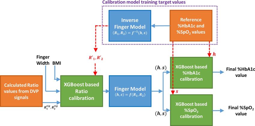
www.nature.com/scientificreports/
Many methods are employed to estimate blood glucose and glycated hemoglobin levels. Over the past few
decades, many enzymatic and nonenzymatic electrochemical glucose sensors have also been d eveloped10–15, but
these methods are invasive. In contrast, noninvasive glucose estimation is a comparatively new topic, although
some of its implementations using external bodily tissues (skin tissues) and fluids (e.g., saliva and tears) have
been reported16,17. Implementations of PPG signals for blood glucose level estimation have also been presented6.
The four most common methodologies used for HbA1c estimation are immunoassay, ion-exchange high-
performance liquid chromatography (HPLC), boronate affinity chromatography, and enzymatic assays18. These
methodologies require a whole blood sample and are performed by different chemical and/or electrochemical
means. However, to date, noninvasive in-vivo research methodologies have not yet been performed to estimate
the percent measurement of the %glycated hemoglobin. A noninvasive classification-based solution (classification
among diabetic, obese, and normal control groups) has been applied to mice models by measuring hypergly-
cemia-associated conditions19. One study discussed the estimation of in vitro glycated hemoglobin (HbA1c)20,
but only focused on the PPG sensor design and did not address noninvasive in-vivo estimation methods. Other
conference papers, which also focused on the classification of a person’s diabetic status, did not perform estima-
emoglobin21,22. Another paper focused on breath acetone-based HbA1c e stimation23, but the
tion of glycated h
error rate was very high.
In this study, glycated hemoglobin (HbA1c) is estimated through an optical plethysmographic system. A
single white light is transmitted through the fingertip, and the transmitted light waves of different wavelengths
are received with three different optical filters on the optical sensor side. This received light wave is called the
DVP signal.
The %HbA1c in the blood is estimated along with the %SpO2 value using this received DVP signal of multiple
wavelengths of light. The DVP signals of three wavelengths are taken to perform this research and estimate the
two abovementioned parameters.
Contrary to the related works described above, which mainly focused on categorizing glycemic levels or
assessing diabetic status, this study focuses on the percent estimation of in-vivo glycated hemoglobin levels.
These percent glycated hemoglobin levels can be used to control the HbA1c levels of normal people, as well
as prediabetic and diabetic patients. Furthermore, this study involves DVP signals that are easy to acquire and
require low-cost devices. This allows the wearable device to be configured to estimate the glycated hemoglobin
levels on-demand or in a continuous manner, noninvasively. Along with all these advantages, the application
of this method can be considered a potential low-cost and accurate glycated hemoglobin estimation device.
Gray‑box model
In mathematics and computational models, the gray-box models have a special role. This model can explain
how the whole system operates (like a white-box model), and on the other hand, it also corresponds with the
practical reference data matched statistically. Therefore, a gray-box model is a combination of theoretical parts,
as well as the data-based black-box model. Here, in this study, we develop theoretically based models based on
the physiology of blood transportation and glycation of hemoglobin and combined this model with black-box
calibration models.
Finger models and coefficients
Glycated hemoglobin or HbA1c was estimated herein through an optical sensor and transmitter system. Multiple
light waves were transmitted through the fingertip, and the transmitted light waves (for a transmissive system)
were recorded with an optical sensor. These recorded signals are called the DVP signals.
Using the DVP signal received from multiple light sources, we calculated the percent glycated hemoglobin
(%HbA1c) in the blood along with the percent oxygen saturation (%SpO2). These two parameters were estimated
at the same time; hence, three light sources were required (i.e., 525, 465, and 615 nm denoted by 1, 2, and 3,
respectively). According to this physiological basis gray-box model-based approach, any three different wave-
lengths of light can be chosen. However, these wavelengths were chosen to easily implement these models with
a simple color sensor. It is also possible to utilize a mobile camera sensor to record DVP signals.
The location of the DVP signal acquisition (e.g., fingertip, upper and lower wrists, earlobe, etc.) was modeled
as a simple mathematical model of only the blood components for the first model and the homogenous mixture
of tissues, arterial and venous blood, and water for the second model, which is the whole-finger model. The bones
were ignored because we assumed that the bone tissues would not transmit enough light to be detected by the
optical sensor. The assumption states the bone as a fixed perfect absorber of light contributing to the DC parts of
the signal only. The abovementioned models stated the blood as a homogenous mixture of glycated hemoglobin
(HbA1c), oxygenated hemoglobin (HbO), and reduced deoxygenated hemoglobin (HHb).
%HbA1c and %SpO2 are described as follows:
cHbA1c
%HbA1c =
cHHb + cHbO + cHbA1c
× 100% , (1)
cHbO
%SpO2 =
cHHb + cHbO
× 100% , (2)
where, cHbA1c , cHbO , and cHHb are the molar concentrations of HbA1c, HbO, and HHb, respectively. The denomi-
nator of %SpO2 does not include cHbA1c or any other components because the base for %SpO2 contains only
oxygen-bonded hemoglobin cells and hemoglobin cells available for binding with o xygen24.
Scientific Reports | (2021) 11:12169 | https://doi.org/10.1038/s41598-021-91527-2 2
Vol:.(1234567890)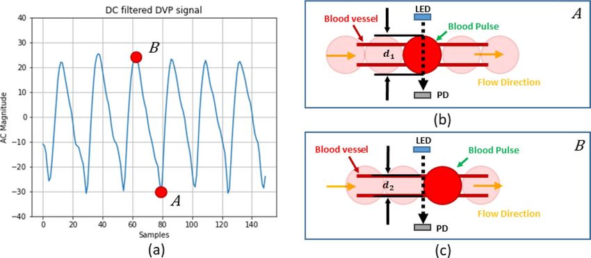
www.nature.com/scientificreports/
Figure 1. Blood-vessel model illustration with hypothetical blood pulses: (a) DVP signal, (b) light intensity
in the systolic phase, and (c) light intensity in the diastolic phase. The variables, d1 and d2 are the diameter of
the blood-vessel when blood pulse enters the blood-vessel and leaves the vessel, respectively. In addition, the
photodetector and light emitting diode are denoted as PD and LED, respectively in both (b,c).
The %Glycated hemoglobin and %Oxygen saturation were estimated using two forms of the finger model.
The two models were based on two different hypotheses and described in the following sections.
Blood‑vessel model. The first model was built based on the hypothesis that when blood comes into the
blood-vessel, the diameter of the vessel slightly expands for the incoming blood volume and reduces the diam-
eter when the blood leaves. Figure 1 depicts the blood-vessel model hypothesis.
The first model only considers blood in the blood vessels; thus, the absorption coefficient of the homogenous
mixture of the HbA1c, HbO, and HHb blood components can be calculated as
Ca = ǫaHbA1c ( ) × cHbA1c + ǫaHbO ( ) × cHbO + ǫaHHb ( ) × cHHb , (3)
Therefore, Ca = µHbA1c
a ( ) + µHbO
a ( ) + µHHb
a ( ). (4)
In Eq. (3), C
a is the total absorption coefficient of the model solution;
ǫ is the molar absorption coefficient
L mol−1 cm−1 ; c is the molar concentration of the attenuator mol L−1 . In Eq. (4), µHbA1c a , µHbO
a , and µHHb
a
are the absorption coefficients, while ǫaHbA1c ( ), ǫaHbO ( ), and ǫaHHb ( ) are the molar absorption coefficients of
HbA1c, HbO, and HHb, respectively.
Whole‑finger model. The whole-finger model was constructed based on the homogenous mixture of the
lumped finger elements (e.g., dermal tissue, water, and arterial and venous blood). Similar to the previous model,
blood is also considered a homogenous mixture of HbA1c, HbO, and HHb hemoglobin cells. Figure 2 illustrates
the fractional volume composition of the whole-finger model.
The absorption coefficient of the finger elements can be calculated as
Ca = Va µart vein water
a ( ) + Vv µa ( ) + Vw µa ( ) + [1 − (Va + Vv + Vw )]µbaseline
a , (5)
where, µart HHb
a = µa
art
+ PHbO µHbO
a − µHHb
a
art
+ PHbA1c µHbA1c
a − µHHb
a , (6)
µvein
a = µHHb
a
vein
+ PHbO µHbO
a − µHHb
a
vein
+ PHbA1c µHbA1c
a − µHHb
a . (7)
In Eq. (5), Va, Vv , and Vw are the partial volume fractions of the artery, vein, and water, respectively; and µarta ,
a , µa
µvein water , and µbaseline are the absorption coefficients of the arterial composition, venous composition, water,
a
and lumped dermal skin layer, respectively. In Eqs. (6) and (7), the µHHb a , µHbO
a , and µHbA1c
a are not the true
absorption coefficients of deoxy-, oxy-, and glycated-hemoglobin. These are the results of the multiplication of
the molar absorption coefficient of respective hemoglobin types with whole blood concentration. PHbO art , P art
HbA1c ,
vein , and P vein are the partial molar concentrations of HbO and HbA1c in the artery and vein, respectively.
PHbO HbA1c
They can be mathematically stated as
Scientific Reports | (2021) 11:12169 | https://doi.org/10.1038/s41598-021-91527-2 3
Vol.:(0123456789)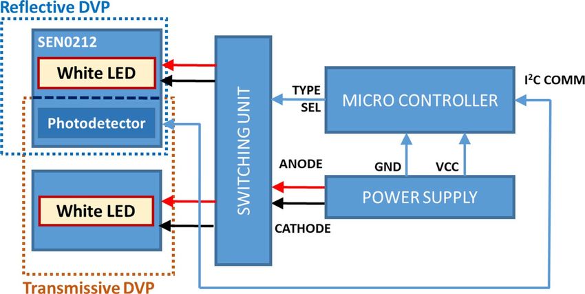
www.nature.com/scientificreports/
Figure 2. Fractional volume composition of the whole-finger model.
cHbO
PHbO =
cHHb + cHbO + cHbA1c
, (8)
cHbA1c
PHbA1c =
cHHb + cHbO + cHbA1c
, (9)
PHHb = 1 − (PHbO + PHbA1c ), (10)
where PHHb represents the partial molar concentration of HHb(deoxy hemoglobin). Equations (6) and (7) can be
easily derived from the following form (refer to Sect. 1 of the Supplementary Document for detailed derivation):
µa = ǫaHbA1c ( ) × cHbA1c + ǫaHbO ( ) × cHbO + ǫaHHb ( ) × cHHb ,
µa = (cTot )× ǫaHHb + PHbO ǫaHbO − ǫaHHb + PHbA1c ǫaHbA1c − ǫaHHb , [From (8), (9), and (10)],
where, cTot = cHbA1c + cHbO + cHHb = 64500 150
mol dm−3 .
Equations (8) to (10) have the same structure for both artery and vein locations. The molar concentration
values in the abovementioned equations were changed according to the location (i.e., artery or vein). The value
of the total concentration of blood, cTot is considered 150/64,500 mol/dm3. This value is the typical molar con-
centration of whole blood. Using the partial molar concentration terminologies (i.e., PHbA1c , PHbO , andPHHb) as
described above, the %HbA1c and %SpO2 formulas in Eqs. (1) and (2) can be redefined as follows:
PHbO
%SpO2 = × 100%, (11)
PHHb + PHbO
%HbA1c = PHbA1c × 100%. (12)
Beer–Lambert law
When blood enters a blood vessel in a certain region, the incident light is absorbed differently compared to the
region with no blood because different blood components also absorb light differently. The total absorbance of
a homogeneous solution can be mathematically described by the Beer-Lambert Law as follows:
N N
I
A= Ai = ǫi × ci × d = − log , (13)
I0
i=1 i=1
where A is the total absorbance
of the solution; N is the number of attenuating species;
ǫ is the molar absorp-
tion coefficient L mol−1 cm−1 ; c is the molar concentration of the attenuating species mol cm−1 ; and d is the
distance traversed by the light beam inside the specimen.
Scientific Reports | (2021) 11:12169 | https://doi.org/10.1038/s41598-021-91527-2 4
Vol:.(1234567890)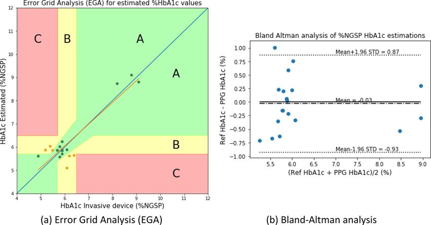
www.nature.com/scientificreports/
Figure 3. Parameter estimation with the Beer–Lambert law.
The absorbance of the solution obtained by the Beer-Lambert Law can be directly measured by applying
the incident light ( I0) and measuring the intensity of the light transmitted by the solution ( I ). Therefore, if any
homogeneous solution can be represented in the form of (13), it can be solved for an unknown parameter.
The Beer-Lambert Law can be applied to the previously described finger models to obtain the total absorb-
ance of the model solution. The decadic absorption coefficient described in the finger model Eqs. (3) to (5) can
be described in terms of absorbance (A) in the following form because the solution is considered homogeneous
and will have a uniform absorption along the light traversal path. Figure 3 depicts the parameter estimation
utilizing the Beer–Lambert law.
A = Ca d. (14)
Blood‑vessel model. The following were obtained when solving the blood-vessel model from Eqs. (3) and
(14):
A = ǫaHbA1c ( ) × cHbA1c + ǫaHbO ( ) × cHbO + ǫaHHb ( ) × cHHb × d. (15)
According to this current hypothesis, the molar concentration of the individual components of the model
solution will be the same, even when blood comes into the vessels, increasing the volume of the vessel tracts.
Therefore, in this assumption, the distance traversed by the light beam inside the finger model will be increased
when blood comes in and will be reduced when blood leaves the vessel.
In other words, if absorbance is measured in the two states (i.e., when blood comes in [ A1] and flows out [ A2
]), the difference between the two states is obtained as
δA = ǫaHbA1c ( ) × cHbA1c + ǫaHbO ( ) × cHbO + ǫaHHb ( ) × cHHb × δd, (16)
where
δd = d1 − d2 , δA = A1 − A2 .
For the three light wavelengths (i.e., 1, 2, and 3), Eq. (16) can be written as
δA 1 = ǫaHbA1c ( 1 ) × cHbA1c + ǫaHbO ( 1 ) × cHbO + ǫaHHb ( 1 ) × cHHb × δd, (17)
δA 2 = ǫaHbA1c ( 2 ) × cHbA1c + ǫaHbO ( 2 ) × cHbO + ǫaHHb ( 2 ) × cHHb × δd, (18)
δA 3 = ǫaHbA1c ( 3 ) × cHbA1c + ǫaHbO ( 3 ) × cHbO + ǫaHHb ( 3 ) × cHHb × δd. (19)
From Eqs. (17) to (19), three ratio equations can be obtained, and any two ratio equations can be used to
estimate the two unknowns, %HbA1c and %SpO2. For convenience, we now define two ratio equations as follows:
Scientific Reports | (2021) 11:12169 | https://doi.org/10.1038/s41598-021-91527-2 5
Vol.:(0123456789)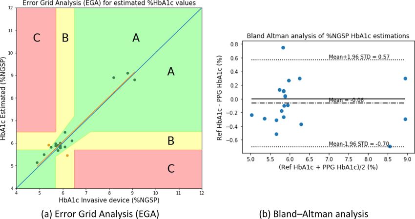
www.nature.com/scientificreports/
δA 1 ǫ HbA1c ( 1 ) × cHbA1c + ǫaHbO ( 1 ) × cHbO + ǫaHHb ( 1 ) × cHHb
R1 = = aHbA1c , (20)
δA 3 ǫa ( 3 ) × cHbA1c + ǫaHbO ( 3 ) × cHbO + ǫaHHb ( 3 ) × cHHb
δA 2 ǫ HbA1c ( 2 ) × cHbA1c + ǫaHbO ( 2 ) × cHbO + ǫaHHb ( 2 ) × cHHb
R2 = = aHbA1c . (21)
δA 3 ǫa ( 3 ) × cHbA1c + ǫaHbO ( 3 ) × cHbO + ǫaHHb ( 3 ) × cHHb
To represent Eqs. (20) and (21) with the %SpO2 and %HbA1c terms, the equations can be simplified with
PHbA1c , PHbO , and PHHb terms from Eqs. (8) to (10). The solved PHbO and PHbA1c terms can then be easily con-
verted to the %SpO2 and %HbA1c terms, respectively, using Eqs. (11) and (12).
Thus, applying Eqs. (8) to (10) to Eqs. (20) and (21), we obtain:
PHbA1c ǫ HbA1c ( 1 ) − ǫ HHb ( 1 ) + PHbO ǫ HbO ( 1 ) − ǫ HHb ( 1 ) + ǫ HHb ( 1 )
R1 =
, (22)
PHbA1c ǫ HbA1c ( 3 ) − ǫ HHb ( 3 ) + PHbO ǫ HbO ( 3 ) − ǫ HHb ( 3 ) + ǫ HHb ( 3 )
PHbA1c ǫ HbA1c ( 2 ) − ǫ HHb ( 2 ) + PHbO ǫ HbO ( 2 ) − ǫ HHb ( 2 ) + ǫ HHb ( 2 )
R2 =
. (23)
PHbA1c ǫ HbA1c ( 3 ) − ǫ HHb ( 3 ) + PHbO ǫ HbO ( 3 ) − ǫ HHb ( 3 ) + ǫ HHb ( 3 )
The right side of Eq. (13) can be combined with Eqs. (22) and (23) to calculate the ratio equations directly
from the received light from the fingertip and obtain
δA 1 δ − log II0 log II(d
0 (d1 )
1 ) − log II(d
0 (d2 )
2 ) log I(d
I(d
2)
1 )
R1 = =
1 =
1 =
1 , (24)
δA 3 δ − log I log I0 (d1 ) − log I0 (d2 ) log I(d2 )
I0 3 I(d1 ) I(d2 ) 3 I(d1 ) 3
δA 2 log I(d 2)
I(d1 )
Similarly, R2 = =
2 . (25)
δA 3 I(d2 )
log I(d1 )
3
Solving Eqs. (22) and (23) for PHbA1c and PHbO yields:
C1 R1 + C2 R2 + C3
PHbA1c = , (26)
C4 R1 + C5 R2 + C6
C7 R1 + C8 R2 + C9
PHbO = . (27)
C10 R1 + C11 R2 + C12
The coefficients C1 to C12 are the values obtained after solving Eqs. (22) and (23). The values of these coef-
ficients are given in the “Result and comparison between models” section (“PHbA1c and PHbO equations with
coefficient values” section) of this manuscript.
Whole‑finger model. As stated earlier, the whole-finger model considers a homogenous mixture of lumped
fingertip constitutes. The blood coming inside this model will increase the partial volume fraction of the arterial
blood. Simultaneously, the partial volume fractions of the venous blood and water will decrease along with the
baseline skin volume fraction. However, note that these transient changes of the venous, water, and skin com-
ponents were neglected herein for simplicity. The increase in the partial volume fraction of the arterial blood is
denoted by Va. Therefore, only considering the arterial fraction increment, the absorption coefficient equation
becomes
Ca +�Ca = (Va + �Va )µart vein water
a ( )+Vv µa ( )+Vw µa ( )+[1 − (Va + �Va + Vv + Vw )]µbaseline
a .
(28)
The change in the absorption coefficient for the change in the arterial blood volume is denoted by Ca.
Now, subtracting Eq. (5) from Eq. (28), the following is obtained:
�Ca = �Va µart a ( ) − µa
baseline
( ) . (29)
Also, from Eqs. (13) and (14),
I = I0 × 10−Ca d . (30)
Equation (30) needs to be differentiated in terms of Ca to determine the relation of the physical light intensity
with Eq. (29):
dI
= −ln(10)I0 d × 10−Ca d . (31)
dCa
Also,
Scientific Reports | (2021) 11:12169 | https://doi.org/10.1038/s41598-021-91527-2 6
Vol:.(1234567890)
www.nature.com/scientificreports/
Figure 4. Multiple light sources versus multiple sensor filter systems.
dI I
≈ . (32)
dCa Ca
Equations (31) and (32) yield:
�I ≈ −ln(10)I0 �Ca d10−Ca d . (33)
Now, the AC–DC intensity ratio is generated by the assumption IIDC
AC
= II . The AC part of the signal denotes
the pulsatile part of the signal, and vice-versa. Let us then divide Eq. (33) with Eq. (30) and replace Ca from
Eq. (29):
�I
= − ln (10)�Va µart a ( ) − µa
baseline
( ) d. (34)
I
Similar to the previous model, this equation can be used to make the ratio equations of any two of the three
wavelengths. The ratio equations become
�I
µart ( 1 ) − µbaseline ( 1 )
R1 = �I
= aart
I 1 a
baseline ( )
, (35)
I 3
µa ( 3 ) − µa 3
�I
I 2 µart baseline ( )
a ( 2 ) − µa 2
R2 = �I
= . (36)
I 3
µart baseline ( )
a ( 3 ) − µa 3
Finally, solving Eqs. (35) and (36) gives two equations with the following forms:
art C1 R1 + C2 R2 + C3
PHbA1c = , (37)
C4 R1 + C5 R2 + C6
art C7 R1 + C8 R2 + C9
PHbO = . (38)
C10 R1 + C11 R2 + C12
The coefficients C1 to C12 are the values obtained after solving Eqs. (35) and (36). The values of these coef-
ficients are given in the “Result and comparison between models” section (“PHbA1c and PHbO equations with
coefficient values” section) of this manuscript.
Data acquisition and processing methodology
A system was designed to acquire the DVP signals from the volunteers and perform experiments on these
mathematical models. As the theory for the Beer-Lambert Law states, the nature of the DVP system should be
transmissive. Thus, for the fingertip DVP acquisition, the light sources should be on one side of the fingertip,
and the sensor should be on the other side. The light rays should pass the fingertip and be received by the sensor.
For this reason, a high-intensity light source is required to detect a good-quality signal.
This model depended on three different wavelengths for the same signal; hence, an RGB color sensor and
a white light for the light source were utilized. The color sensor had three different filters on top of the sensor
die: blue (465 nm), green (525 nm), and red (615 nm). Clear (i.e., no filter) regions were also present on the
sensor. Hence, the space constraint problem in the transmissive DVP system for the light source was solved.
Instead of using three high-intensity light sources of different wavelengths, only one white light source and
three-wavelength light filters were used on the sensor side (Fig. 4). Figure 5 depicts a basic diagram of the signal
acquisition device. In addition to the DVP data, the HbA1c and SpO2 reference data were also taken to calibrate
and validate these models.
The microcontroller used in this study is Arduino Uno as depicted in Fig. 5. The commercial sensor module
DFRobot SEN0212 comprises a color sensor (TCS34725) and a set of four white LEDs. TCS34725 is a highly
Scientific Reports | (2021) 11:12169 | https://doi.org/10.1038/s41598-021-91527-2 7
Vol.:(0123456789)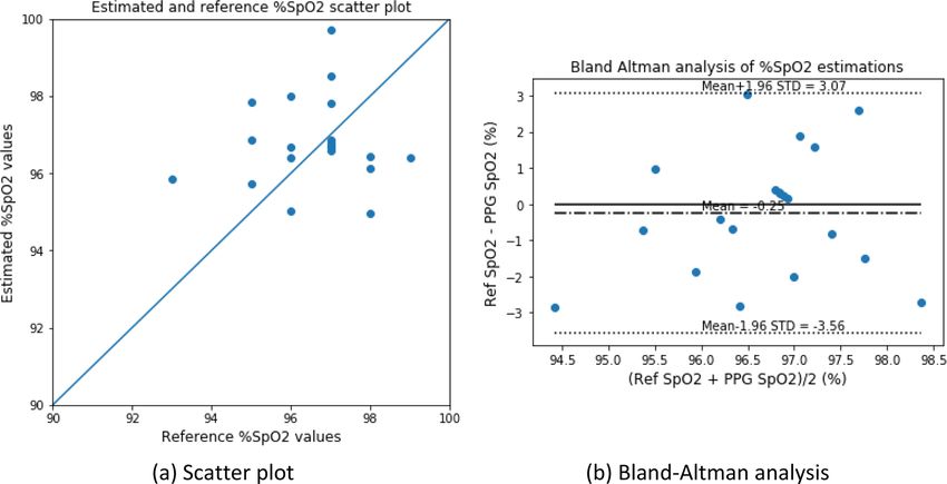
www.nature.com/scientificreports/
Figure 5. DVP signal acquisition device block diagram.
Figure 6. Illustration of (a) sensor module-LED arrangement and (b) physical image of the device.
sensitive sensor with three wavelengths. The wavelengths include 465, 525, and 615 nm. This sensor can run at
about 37 Hz sampling rate over the I 2C protocol.
The white LEDs with the sensor module are placed around the photodetector. These LEDs are used for
recording reflective DVP. For recording transmissive DVP signals, a discrete high-power white LED is attached
to the device. The switching unit delivers power to only one of the LEDs (transmissive or reflective) based on
the “Type Sel” signal from the microcontroller. The “Type Sel” signal is altered each 1 min to switch the device
to change the mode (transmissive or reflective) of the device. For this study, only the transmissive DVP signal
was used. The LED and sensor module are attached to a clip-type fingertip device. Figure 6 illustrates the LED-
sensor module arrangement in the clip type device and physical device image.
The SEN0212 sensor module (PD and reflective LEDs) is kept in the soft tissue side of the finger, whereas the
transmissive white LED is placed over the fingernail as shown in Fig. 6. This arrangement is kept constant for
taking data from all the participants.
The Arduino Uno microcontroller is connected to a PC for recording the DVP data. The microcontroller
takes the sensor module data and transmits the data via USB serial connection with the PC. This serial data is
then saved as comma-separated value (CSV) text files.
These CSV files are then taken into a Python program to preprocess the waveform and calculate the HbA1c
and SpO2 values with the equations and calibration procedure described in the subsequent subsections.
The preprocessing of the waveforms includes filtering the waveforms with a second-order Butterworth low-
pass filter with a cutoff frequency at 8 Hz. Then, calculate the ratio values with the equations described in the
next section. After that, numeric error values and infinite number values are removed from the calculated ratio
values. Finally, to remove the effects of noisy signal and miscalculations, data points in the 60% confidence
interval (CI) around the mean are taken as the filtered ratio values.
After the preprocessing of the data, the data is fed into the system to evaluate and calibrate the XGBoost
models using the leave-one-out-cross-validation (LOOCV) technique. The detailed system description and
calibration process are described in the calibration subsection of the following section.
Scientific Reports | (2021) 11:12169 | https://doi.org/10.1038/s41598-021-91527-2 8
Vol:.(1234567890)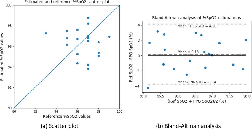
www.nature.com/scientificreports/
Molar absorption coefficient
(M−1 cm−1)
Wavelength (nm) HbA1c HbO HHb
465 549,024.7353 38,440.2 18,701.6
525 455,139.5677 30,882.8 35,170.8
615 170,555.4218 1166.4 7553.4
Table 1. Molar absorption coefficient of HbA1c, HbO, and HHb for the respective wavelengths.
Absorption coefficient (cm−1)
Wavelength (nm) HbA1c HbO HHb Skin baseline Water
465 1276.8017 89.3958 43.4921 1.6279 0.00020277
525 1058.4641 71.8205 81.7926 1.0966 0.0003927
615 396.6405 2.7126 17.566 0.6552 0.0027167
Table 2. Absorption coefficients of HbA1c, HbO, HHb, skin baseline, and water for the respective light
wavelengths.
Human participant ethical compliance. We have compiled ethical regulations for our research meth-
odology from the Institutional Review Board (IRB), Kookmin University, Seoul, Korea. This research was con-
ducted in accordance with the guidelines provided by the IRB, Kookmin University. And we also have obtained
informed consent from all the participants for utilizing the data obtained from them, for academic research
purposes.
Result and comparison between models
Coefficient values on different wavelengths. The data acquisition device used three dominant wave-
lengths of 465, 525, and 615 nm; thus, the values of the wavelength-dependent parameters for the respective light
wavelengths must be evaluated to solve the model equations. These parameters include the molar absorption
coefficient of HHb, HbO, and HbA1c given in Table 1 and the absorption coefficient of HHb, HbO, HbA1c, skin
baseline, and water given in Table 2. The molar absorption coefficient data of HbA1c were taken from studies
by Hossain et al.25 and HbO and HHb were taken from P rahl26, respectively. The absorption coefficient data of
HbA1c, HbO, and HHb were calculated from the molar absorption coefficient multiplied by 150/64,500 mol/L
for the whole blood hemoglobin. The absorption coefficient data of the skin baseline and water were taken from
studies by Saidi27 and S egelstein28, respectively.
The absorption coefficient values of HbA1c, HbO, and HHb described in Table 2 are not true absorption
coefficients of those parameters. Rather, they are the multiplication of molar absorption coefficients of respective
elements with the whole-blood molar concentration.
Ratio equations with coefficient values. For the blood-vessel model, the following equations were
obtained by taking the wavelength ( ) values as 1 = 525nm, 2 = 465nm, and 3 = 615nm and placing the
parameter values from Table 1 into Eqs. (22) and (23):
419968.1653 × PHbA1c − 4288.0 × PHbO + 35170.8
R1 = , (39)
163002.0218 × PHbA1c − 6387.0 × PHbO + 7553.4
530323.1353 × PHbA1c + 19738.6 × PHbO + 18701.6
R2 = . (40)
163002.0218 × PHbA1c − 6387.0 × PHbO + 7553.4
The following equations were acquired by defining similar wavelength ( ) values for the whole-finger model
and placing the values from Table 2 into Eqs. (35) and (36):
976.6715 × PHbA1c − 9.9721 × PHbO + 80.696
R1 = , (41)
379.0745 × PHbA1c − 14.8534 × PHbO + 16.9108
1233.3096 × PHbA1c + 45.9037 × PHbO + 41.8642
R2 = . (42)
379.0745 × PHbA1c − 14.8534 × PHbO + 16.9108
PHbA1c and PHbO equations with coefficient values. At this stage, Eqs. (39) to (42) were solved for
PHbA1c and PHbO . For the blood-vessel model, Eqs. (39) and (40) were solved, and equations were obtained in the
form of Eqs. (26) and (27) with the coefficient values given in Table 3.
Scientific Reports | (2021) 11:12169 | https://doi.org/10.1038/s41598-021-91527-2 9
Vol.:(0123456789)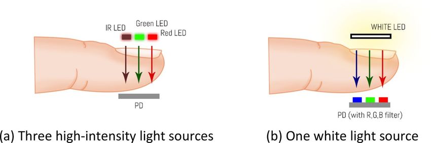
www.nature.com/scientificreports/
c1 c2 c3 c4 c5 c6
13.427 − 9.612 − 38.721 − 330.230 99.169 528.181
c7 c8 c9 c10 c11 c12
− 47.867 − 128.036 539.890 − 330.230 99.169 528.181
Table 3. Coefficient values for the PHbA1c . and PHbO equations of the blood-vessel model.
c1 c2 c3 c4 c5 c6
1.398 − 1.030 − 4.122 − 35.720 10.727 57.132
c7 c8 c9 c10 c11 c12
− 4.987 − 14.073 58.636 − 35.720 10.727 57.132
Table 4. Coefficient values for the PHbA1c and PHbO equations of the whole-finger model.
Figure 7. Dataset diabetes class plot.
Similarly, for the whole-finger model, Eqs. (41) and (42) were solved in the form of Eqs. (37) and (38), with
the coefficients given in Table 4.
Clinical dataset information. A small “proof of method” test with 20 participants was conducted to test
the hypothesis and model performance. Four volunteers were normal, 13 were in the prediabetic range, and 3
had diabetes (Fig. 7). The age range of the subjects was from 25 to 55 years (31.6 ± 10). Among the subjects, 5
of them were females and 15 of them were males. The mean and standard deviation (SD) ( Mean ± SD ) of finger
width and BMI of our dataset are 1.30 ± 0.13 and 28.86 ± 3.74, respectively. Refer to Sect. 8 of the Supplemen-
tary Document for complete dataset information.
For each volunteer, 4 min of DVP was recorded, and SpO2 data and a National Glycohemoglobin Standardi-
zation Program (NGSP) %HbA1c value were measured using an invasive device. The S pO2 data were acquired
using the Schiller Argus OXM Plus clinical blood oxygenation patient-monitoring device, whereas the invasive
%NGSP HbA1c was measured using the BioHermes A1C EZ 2.0 device.
Within the 4 min of recorded DVP signal, 2 min were transmissive DVP signal and the other 2 min were
reflective DVP signal. Since the theoretical derivation described above was only on the transmissive DVP signal,
the 2 min transmissive DVP signal was used to perform the experiments.
Ethical regulations were compiled for the research methodology from the Institutional Review Board (IRB),
Kookmin University, Seoul, Korea. This study was conducted in accordance with the guidelines provided by the
IRB, Kookmin University. In addition, prior consent was obtained from all participants in order to utilize the
data obtained for academic research purposes.
Any normal and self-reported diabetic volunteers aged 19 to 65 were set to participate in this study. Prospec-
tive volunteers were notified to the IRB committee of Kookmin University.
The volunteers were first checked for any known previous complications that might cause problems either
to them or to the experiment. The complications include any record of low blood volume (hypovolemia) and
irregular heart rate (tachycardia) within the range of a month. They were then asked to sit idly for approximately
1 to 2 min to stabilize their heart rate. Subsequently, the DVP waveform was recorded from the index finger of
the participants with the corresponding devices. The S pO2 parameter of a volunteer was recorded in video format
from the Argus device display. The volunteers were steady at the time of data acquisition; thus, the variability
Scientific Reports | (2021) 11:12169 | https://doi.org/10.1038/s41598-021-91527-2 10
Vol:.(1234567890)www.nature.com/scientificreports/
Figure 8. Histogram plot of the measured dataset (a) %NGSP HbA1c value and (b) %SpO2 value.
Min Max Mean Median SD Variance 25th Percentile 75th Percentile
%HbA1c 4.9 9.1 6.22 5.9 1.103 1.216 5.7 6.125
%SpO2 93 99.0 96.55 97.0 1.322 1.747 96.0 97.0
Table 5. Statistics of the measured %HbA1c and %SpO2 data.
of blood oxygen saturation was very low. Due to the S pO2 invariability, the average of the blood oxygen satura-
tion values was taken for each individual to evaluate the model. Figure 8 depicts the distribution of the %NGSP
HbA1c and %SpO2 values for the dataset. Table 5 presents the statistics of the %NGSP HbA1c and %SpO2 values.
Calibration. After dataset creation and data preprocessing, the model was now calibrated with experimental
data. These models were based on simple assumptions and processes. Consequently, the models will eventually
generate erroneous values without calibration due to model inaccuracy.
The calibration process of this system is performed in two steps. In the first step, the calculated ratio values
from the acquired DVP signal are calibrated. In the second step, the calculated HbA1c and S pO2 values are
calibrated to get more accurate estimations. Each of these calibrations is performed with the XGBoost Regres-
sion algorithm. The description of each calibration step is given in the subsequent paragraphs followed by the
description of dataset splitting, training–testing, and scoring procedures.
To calibrate each of these models, it was assumed that the measured %NGSP HbA1c and %SPO2 values were
correct. Based on this assumption, the recorded DVP signal values were first adjusted by calibrating the two
sig sig
ratio values ( R1 and R2 ) obtained from the signal amplitudes with the calculated ratio values (R1′ and R2′ ) from
reference %HbA1c and %SpO2 values. The ratio values from the DVP signal are calculated from light intensity
expressions of Eqs. (24) and (25) for blood-vessel model and Eqs. (35) and (36) for the whole-finger model,
respectively. The calculated ratio values and deducted from Eqs. (39) and (40) for the blood-vessel model and
Eqs. (41) and (42) for the whole-finger model gave the normalized values of the measured reference %HbA1c
and %SpO2. This step of calibrating the ratio values is crucial because different individuals have different finger
widths and different skin and fat layer properties. To reduce the effects of skin, fat layer, and finger width effects
on DVP signal amplitudes, this calibration process is applied. In this calibration step, the ratio values from the
signal are calibrated to calculated ratio values ( R1′ and R2′ ) from Eqs. (39) to (42) with two more features that
can compensate for the ratio variability among individuals. The two features are finger width and body mass
sig sig
index (BMI). Therefore, there are four input features, R1 , R2 , finger width, and BMI. The targets are R1′ and R2′
for two independent ratio calibrators, respectively. Refer to Sects. 3 and 4 of the Supplementary Document for
feature importance metrics for different input features in the ratio calibration step. Furthermore, Sect. 5 of the
Supplementary Document contains the analysis of the calibrated ratio values for a different set of input features.
After calibrating the ratio values, the finger model equations were used to estimate the normalized Hba1c and
SpO2 values. Although these values were close to the reference measurements, these required further calibration
to mitigate the model errors (i.e., model inadequacy and propagation errors). This second-level calibration was
done on the calculated HbA1c and S pO2 values given the reference HbA1c and S pO2 as targets, respectively.
Refer to Sects. 6 and 7 of the Supplementary Document for a detailed analysis of the impacts of features on the
estimation of HbA1c levels. Both calculated HbA1c and S pO2 values were provided as the inputs to the calibration
model. The reference HbA1c and reference S pO2 values were considered as the target values for the respective
value calibration models.
The training and testing of these calibration models were performed with leave-one-out-cross-validation
(LOOCV) technique. This is a modified K-fold cross-validation technique, in which the number folds are equal
to the number of participants in our study. In each fold, the data from one participant is set to test the model,
Scientific Reports | (2021) 11:12169 | https://doi.org/10.1038/s41598-021-91527-2 11
Vol.:(0123456789)www.nature.com/scientificreports/
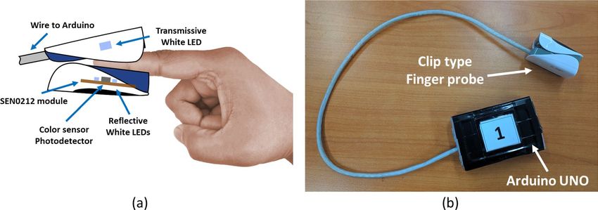
Figure 9. Proposed system overview diagram with calibration blocks. (h = normalized HbA1c, s = normalized
SpO2). The blue lines indicate the flow of data, and the red dotted lines indicate the target value for training the
calibration models. The target values are absent in the testing phase.
whereas the other participants’ data are provided to train the model. The patient for testing the model is chosen
randomly, and each participant’s data are set to be tested exactly once.
To train the XGBoost calibration models in each, the reference %NGSP HbA1c and S pO2 values of the training
cohort are required (Sect. 2 of the Supplementary Document describes the XGBoost model training parameters).
In contrast, the testing of the model is free from reference HbA1c and SpO2 values. These test results are used
for further processing in the system or given as final estimation results and for scoring the estimated results. The
block diagram of the overall system overview with the calibration model blocks is shown in Fig. 9.
In Fig. 9, the orange blocks represent the reference and input data sources, the green blocks represent calibra-
tion steps, and the blue blocks represent finger models. The calibrator models’ training target values are drawn
with dashed red lines, and the inputs are drawn with solid blue lines. The “Inverse Finger Model” and “Reference
%HbA1c and %SpO2 values” blocks are only required for the dataset of the training cohort in each fold of the
LOOCV. For testing the overall system, the reference blocks are not required. The calibrated ratio values using
XGBoost regressor with LOOCV test results are passed to the finger model to estimate the normalized HbA1c
and SpO2 values. Then these estimated normalized HbA1c and SpO2 values are again calibrated and the LOOCV
test results are considered as the final estimated %HbA1c and %SpO2 values.
Result deduction. The following results were obtained with the two models after %HbA1c value calibra-
tion: the plot of Clarke’s error grid analysis (EGA)29,30 is given with the Bland–Altman analysis in Fig. 10 for the
blood-vessel model and Fig. 11 for the whole-finger model.
Figure 10 illustrates that the error grid analysis, with Zone A (clinically accurate data) containing 14 samples
(73.68%), Zone B containing 5 samples (26.31%; data outside of 20% of the reference, but would not lead to
inappropriate treatment), and Zone C with 0 (0%; data that would lead to uncertain treatment). Figure 11 shows
the whole-finger model consisting of 18 (90.0%), 2 (10.0%), and 0 (0%) samples in zones A to C, respectively.
The Bland–Altman analysis indicated that the blood-vessel model provided a bias of – 0.03 ± 0.458, and the
limits of agreement (95%; 1.96 SD) ranged from − 0.93 to 0.87. For the whole-finger model, the bias was – 0.06 ±
0.326, and the limits of agreement ranged from − 0.70 to 0.57. The limits of agreement of the whole-finger model
were smaller than that of the blood-vessel model.
The prediction repeatability was also tested for each patient’s data. Two minutes of the transmissive DVP
data were taken; thus, the percent coefficient of variation (%CV) for the predicted %NGSP HbA1c for each
data frame (single DVP wave) for each patient is indicated as a measure of the repeatability in the full 2 min of
transmissive DVP data. Figure 12 depicts the %CV versus reference %HbA1c data. To estimate the %CV for
each participant’s data, all the data frames of a single participant are individually fed into this system to estimate
the HbA1c and S pO2 values. Then the %CV of the corresponding parameter (i.e., HbA1c or S pO2) is calculated
with these estimated values.
The %CV plot of all data frames illustrates that the mean %CV was 2.08% for the blood-vessel model and
1.74% for the whole-finger model. These results are very accurate for the repeatability analysis.
The statistical analysis of the estimated and reference %HbA1c data from the blood-vessel model yielded the
mean square error (MSE) of 0.211, mean error (ME) of − 0.031, mean absolute deviation (MAD) of 0.375, and
root mean square error (RMSE) of 0.459. The Pearson’s R coefficient metric was 0.916.
Similarly, the statistical analysis of the whole-finger model provided 0.110, − 0.065, 0.271, and 0.332 for the
MSE, ME, MAD, and RMSE, respectively. The Person’s R coefficient metric was 0.959.
Scientific Reports | (2021) 11:12169 | https://doi.org/10.1038/s41598-021-91527-2 12
Vol:.(1234567890)www.nature.com/scientificreports/
Figure 10. HbA1c Clarke’s error grid analysis (EGA) and Bland–Altman analysis for the blood-vessel model.
Figure 11. HbA1c Clarke’s error grid analysis (EGA) and Bland–Altman analysis for the whole-finger model.
The estimated %SpO2 values were also calibrated and analyzed. Figures 13 and 14 depict the scatter plot and
the Bland–Altman analysis of the estimated versus reference %SpO2 values for the blood-vessel and whole-finger
models, respectively. The Bland–Altman analysis of the %SpO2 values showed a bias of 0.178 ± 2.002 and – 0.246
± 1.690 for the blood-vessel and whole-finger models, respectively. The limit of agreement ranged from − 3.74 to
4.10 and − 3.56 to 3.07 for the models, respectively.
For the repeatability analysis of the estimated %SpO2 values, the %CV was calculated similarly to the case of
%HbA1c values. The maximum %CV was 1.58 and 1.77 for the blood-vessel and whole-finger models, respec-
tively, whereas the mean %CV was 0.54 and 0.49, respectively (Fig. 15).
The statistical analysis with MSE, ME, MAD, and RMSE for the estimated %SpO2 values gave 4.038, 0.178,
1.676, and 2.010 for the blood-vessel model and 2.924, − 0.246, 1.395, and 1.710 for the whole-finger model. The
reference closeness factor (RCF) was found to be 0.983 and 0.986, respectively, for the two models.
The RCF is a metric to measure the closeness of the reference and estimated values. This metric is calculated
with the following equation:
Scientific Reports | (2021) 11:12169 | https://doi.org/10.1038/s41598-021-91527-2 13
Vol.:(0123456789)www.nature.com/scientificreports/
Figure 12. Percent coefficient of variation for the reference and estimated %HbA1c values for both models.
Figure 13. Scatter plot and Bland–Altman analysis of the estimated versus reference (measured) %SpO2 values
for the blood-vessel model.
� �
Ref
N �SpO2 (i) − SpO2Est (i)�
� �
1 �
RCF = 1− , (43)
N 100
i=1
Ref
where, N is the total number of samples, and SpO2 and SpO2Est are the reference and estimated %SpO2 levels,
respectively.
Comparison to state‑of‑the‑art methods. Studying the recent studies and state-of-the-art methods
regarding noninvasive in-vivo glycated hemoglobin and blood oxygenation estimation, it can be seen that,
although there are several studies conducted to estimate blood oxygenation, there are very few studies con-
ducted that classify glycated hemoglobin levels in a noninvasive manner. To the best of the authors’ knowledge,
no other research works have been conducted to estimate the percent glycated hemoglobin levels until now. In
this section, the two most notable studies on noninvasive HbA1c are compared based on the methodology and
advancement.
The most notable study in the field of noninvasive in-vivo classification of glycemic status was conducted by
Martín-Mateos et al.19. This study was performed on diabetic mouse models to demonstrate the effectiveness of
categorizing animals with sustained hyperglycemia under nonglycemic conditions using mm-wave transmission
spectroscopy. Although the research illustrated a good approach to categorize glycemic status, it did not estimate
the number of glycation products. Similar work on the classification of glycemic states was also conducted by
Usman et al.22, which utilizes the second derivative of photoplethysmography signals.
Scientific Reports | (2021) 11:12169 | https://doi.org/10.1038/s41598-021-91527-2 14
Vol:.(1234567890)www.nature.com/scientificreports/
Figure 14. Scatter plot and Bland–Altman analysis of the estimated versus reference (measured) %SpO2 values
for the whole-finger model.
Figure 15. Percent coefficient of variation for the reference and estimated %SpO2 values for both models.
Compared to the previous studies, the %HbA1c levels can be accurately estimated by the theoretical deriva-
tion of two different models in our study. This HbA1c can be used to control the blood sugar level for predia-
betic and diabetic patients, which cannot be performed with the methods mentioned above. Furthermore, the
method of the current study makes use of DVP signals, which require low-cost devices, and the signals can be
easily acquired. This can enable the construction of wearable devices capable of estimating the percent glycated
hemoglobin levels in a continuous manner. Along with all these advantages, the application of this method can
be considered as a low-cost instrumentation device for estimating noninvasive glycated hemoglobin having high
potential for commercial applications.
In contrast, most commercial pulse oximeters have absolute mean error (or mean absolute deviation) of less
than 2% at normal saturation (90–97.5% SpO2) and perfusion rate, two-thirds have a standard deviation (SD) of
less than 2%, and the other devices have an SD of less than 3%31. Another research work, also showed a similar
standard deviation of the differences between S aO2 and SpO232. Most devices had a mean of differences (bias)
of up to 2.0%.
Compared to the state-of-the-art blood oxygenation devices, the approach of this study resulted in the S pO2
estimation error bias ( Mean ± SD ) of 0.178 ± 2.002 and – 0.246 ± 1.690, for blood-vessel and whole-finger
models, respectively. From these metrics, it can be said that the estimation accuracy of SpO2 using the system of
this study is comparable with the state-of-the-art noninvasive pulse oximeters. The blood-only model provides
error metrics similar to the industry-standard oximeters, while the whole-finger model provides better accuracy
metrics.
Scientific Reports | (2021) 11:12169 | https://doi.org/10.1038/s41598-021-91527-2 15
Vol.:(0123456789)www.nature.com/scientificreports/
Discussion
The analysis of the volunteers’ data and results evidently showed comparable performance metrics for both
physiological basis gray-box models. The error metrics between the models were similar for the volunteers’
data. The analysis done in these error metrics was based on the mean of a full 2 min of recorded transmissive
DVP data. However, looking at the model estimation repeatability, the blood-vessel model has a higher mean
%CV than the whole-finger model in both cases of %HbA1c and %SpO2 estimations. This can happen due to
the model inaccuracy in the blood-vessel model compared to the whole-finger model. The whole-finger model
takes into account more parameters of the fingertip, rendering the model more accurate in structure compared
to the blood-vessel model. The simpler construction of the blood-vessel model can make it sensitive to the input
noise. Therefore, a photosensor with high sensitivity and lower noise margin should be used to utilize the blood-
vessel model in practical situations.
It is very important to stress that both models are very simple compared to the physical structure of the
fingertip. A physical fingertip differs from person to person in terms of the epidermal, dermal, fat, and muscle
layer thickness and volume. The blood volume also differs due to physical effects or abnormalities. These include
vasoconstriction, vasodilation, and change in blood pressure and perfusion rate. Also, pressure on the measure-
ment site changes the DVP waveform. These parameters highly affect the calculated ratios because these models
cannot consider these uncertainties and might result in high errors. Although this study tried to compensate for
the effects of fat tissues, skin types, and finger width of the individuals’ fingers, some unknown parameters can
always arise to cause regression errors. However, if these models are calibrated for individuals, they should give
a much higher accuracy in the regression analysis as the uncertain parameters are included in the individualistic
calibration process.
It is also important to take note of the variance in the measured reference data. The advertised accuracy
for the Schiller Argus OXM Plus device ( SpO2 monitor) was ± 2% for the 70% to 100% range. In contrast, the
BioHermes A1C EZ 2.0 device (reference HbA1c device) had an advertised precision of %CV of < 3% in the 4.0
to 6.5%HbA1c range. The device manufacturer, however, did not guarantee the precision above and below the
specified range. Our tests showed that the measured %HbA1c value in the range conformed with the advertised
precision value, but above 6.5%, the %CV went close to 4.9% (refer to Sect. 9 of Supplementary Document for
the test details). These inaccuracies in the reference data led to the error propagation in the model parameters
and calibration steps. Taking more patient samples can improve the estimation accuracy greatly for both models.
Conclusion
In this research, two gray-box models with physiological basis assumptions were deduced to estimate the
%HbA1c levels in human blood. The first model only comprised a blood-vessel, whereas the second model
considered a full-finger system for absorption effects only. Although these models are simple compared to the
realistic fingertip structure, upon validation, this study was able to estimate the %NGSP HbA1c and %SpO2 in
clinically accurate regions (region A in EGA plots) in most cases, and the estimation was clinically plausible
(region B in EGA plots) in the other cases for multiple volunteers’ data. No in-vivo non-invasive studies were
previously performed to estimate the percent glycated hemoglobin with digital volume pulse waveform. There-
fore, this study is a strong proof of method in this scope.
Some more factors can be considered in future studies. For example, light scattering in biological media,
finger structure variability, light sources, and detector properties should be examined to obtain better results.
A more controlled calibration can also be performed to reduce the error in the reference data by increasing the
data sample size and improving the data purification algorithm.
Data availability
The dataset used in this research is available upon a valid request to any of the authors of this research paper.
Code availability
The codes used in this study are available in Github (https://github.com/ShifatHossain/hba1c_BLM).
Received: 16 December 2020; Accepted: 21 May 2021
References
1. Temko, A. Accurate heart rate monitoring during physical exercises using PPG. IEEE Trans. Biomed. Eng. 64, 2016–2024 (2017).
2. Chang, H. et al. A method for respiration rate detection in wrist PPG signal using Holo-Hilbert spectrum. IEEE Sens. J. 18,
7560–7569 (2018).
3. Budidha, K., Rybynok, V. & Kyriacou, P. A. Design and development of a modular, multichannel photoplethysmography system.
IEEE Trans. Instrum. Meas. 67, 1954–1965 (2018).
4. Lochner, C. M., Khan, Y., Pierre, A. & Arias, A. C. All-organic optoelectronic sensor for pulse oximetry. Nat. Commun. 5, 1–7
(2014).
5. Shamir, M., Eidelman, L. A., Floman, Y., Kaplan, L. & Pizov, R. Pulse oximetry plethysmographic waveform during changes in
blood volume. Br. J. Anaesth. 82, 178–181 (1999).
6. Jindal, G. D. et al. Non-invasive assessment of blood glucose by photo plethysmography. IETE J. Res. 54, 217–222 (2008).
7. Banik, P. P., Hossain, S., Kwon, T.-H., Kim, H. & Kim, K.-D. Development of a wearable reflection-type pulse oximeter system to
acquire clean PPG signals and measure pulse rate and SpO2 with and without finger motion. Electronics 9, 1905 (2020).
8. World Health Organisation. Global Report on Diabetes (WHO, 2016).
9. Tapp, R. J. et al. Longitudinal association of glucose metabolism with retinopathy: Results from the Australian Diabetes Obesity
and Lifestyle (AusDiab) study. Diabetes Care 31, 1349–1354 (2008).
10. Chen, C. et al. Recent advances in electrochemical glucose biosensors: A review. RSC Adv. 3, 4473–4491 (2013).
Scientific Reports | (2021) 11:12169 | https://doi.org/10.1038/s41598-021-91527-2 16
Vol:.(1234567890)www.nature.com/scientificreports/
11. Bandodkar, A. J. & Wang, J. Non-invasive wearable electrochemical sensors: A review. Trends Biotechnol. 32, 363–371 (2014).
12. Sharma, S., Huang, Z., Rogers, M., Boutelle, M. & Cass, A. E. G. Evaluation of a minimally invasive glucose biosensor for continu-
ous tissue monitoring. Anal. Bioanal. Chem. 408, 8427–8435 (2016).
13. Kagie, A. et al. Flexible rolled thick-film miniaturized flow-cell for minimally invasive amperometric sensing. Electroanalysis 20,
1610–1614 (2008).
14. Li, M., Bo, X., Mu, Z., Zhang, Y. & Guo, L. Electrodeposition of nickel oxide and platinum nanoparticles on electrochemically
reduced graphene oxide film as a nonenzymatic glucose sensor. Sens. Actuators B Chem. 192, 261–268 (2014).
15. Mandal, S., Marie, M., Kuchuk, A., Manasreh, M. O. & Benamara, M. Sensitivity enhancement in an in-vitro glucose sensor using
gold nanoelectrode ensembles. J. Mater. Sci. Mater. Electron. 28, 5452–5459 (2017).
16. Jung, D. G., Jung, D. & Kong, S. H. A lab-on-a-chip-based non-invasive optical sensor for measuring glucose in saliva. Sensors
(Basel) 17, 2607 (2017).
17. Bruen, D., Delaney, C., Florea, L. & Diamond, D. Glucose sensing for diabetes monitoring: Recent developments. Sensors (Basel)
17, 1866 (2017).
18. Little, R. R. & Roberts, W. L. A review of variant hemoglobins interfering with hemoglobin A1c measurement. J. Diabetes Sci.
Technol. 3, 446–451 (2009).
19. Martín-Mateos, P. et al. In-vivo, non-invasive detection of hyperglycemic states in animal models using mm-wave spectroscopy.
Sci. Rep. 6, 34035 (2016).
20. Mandal, S. & Manasreh, M. O. An in-vitro optical sensor designed to estimate glycated hemoglobin levels. Sensors (Basel) 18, 1084
(2018).
21. Usman, S. et al. Second derivative and contour analysis of PPG for diabetic patients. In 2018 IEEE-EMBS Conference on Biomedical
Engineering and Sciences (IECBES) 59–62 (2018). https://doi.org/10.1109/IECBES.2018.8626681.
22. Usman, S., Harun, N., Dziyauddin, R. A. & Bani, N. A. Estimation of HbA1c level among diabetic patients using second derivative
of Photoplethysmography. In 2017 IEEE 15th Student Conference on Research and Development (SCOReD) 89–92 (2017). https://
doi.org/10.1109/SCORED.2017.8305415.
23. Saraoğlu, H. M. & Selvi, A. O. Determination of glucose and Hba1c values in blood from human breath by using radial basis
function neural network via electronic nose. In 2014 18th National Biomedical Engineering Meeting 1–4 (2014). https://doi.org/
10.1109/BIYOMUT.2014.7026340.
24. Zijlstra, W. G. The trouble with properly describing the oxygen-transport-related quantities. https://acutecaretesting.org/en/artic
les/the-trouble-with-properly-describing-the-oxygentransportrelated-quantities. Accessed 29 September 2020.
25. Hossain, S. & Kim, K.-D. Estimation of Molar Absorption Coefficients of HbA1c in Near UV-Vis-SW NIR Light Spectrum (The Korean
Institutes of Communications and Information Sciences, 2020).
26. Prahl, S. A. Tabulated molar extinction coefficient for hemoglobin in water (2005).
27. Saidi, I. S. Transcutaneous optical measurement of hyperbilirubinemia in neonates. PhD dissertation, Rice University, Department
of Bioengineering, January (1992).
28. Segelstein, D. J. The Complex Refractive Index of Water (University of Missouri, 1981).
29. Canchola, J. A. & Canchola, C. M. Using SAS for Error Grid Analysis (EGA) of Glycated Hemoglobin A1c. In Western Users of
SAS Software 2013 (2013).
30. van Raalten, F. et al. Level of agreement of point-of-care and laboratory HbA1c measurements in the preoperative outpatient clinic
in non-diabetic patients who are overweight or obese. J. Clin. Monit. Comput. 33, 1139–1144 (2019).
31. Webb, R. K., Ralston, A. C. & Runciman, W. B. Potential errors in pulse oximetry. Anaesthesia 46, 207–212 (1991).
32. Andersson, K. & Busch Paulsson, E. Accuracy Validation of Pulse Oximeters Used at Hospitals: A Cross-Sectional Study performed
in Stockholm. Masters thesis, KTH Royal Institute of Technology, School of Technology and Health, May (2017).
Acknowledgements
This research was supported by Basic Science Research Program through the National Research Foundation
(NRF) of Korea funded by the Ministry of Education (NRF-2019R1F1A1062317) and was also supported by
the National Research Foundation of Korea Grant funded by the Ministry of Science, ICT, and Future Planning
[2015R1A5A7037615].
Author contributions
S.H. and K.-D.K. conceptualized the work. S.H. conducted the theoretical derivations, data acquisition device
designing, and hardware programming. S.H. and S.S.G. analyzed and purified the reference and input data. S.H.
and S.S.G. conducted the calibration process. The formal analysis was done by T.H.K. and K.-D.K. This whole
work is also supervised by K.-D.K. All authors discussed the results and commented on the manuscript.
Competing interests
The authors declare no competing interests.
Additional information
Supplementary Information The online version contains supplementary material available at https://doi.org/
10.1038/s41598-021-91527-2.
Correspondence and requests for materials should be addressed to K.-D.K.
Reprints and permissions information is available at www.nature.com/reprints.
Publisher’s note Springer Nature remains neutral with regard to jurisdictional claims in published maps and
institutional affiliations.
Scientific Reports | (2021) 11:12169 | https://doi.org/10.1038/s41598-021-91527-2 17
Vol.:(0123456789)You can also read