Demystifying the Costs of Electricity Generation Technologies - World Bank Group
←
→
Page content transcription
If your browser does not render page correctly, please read the page content below
Public Disclosure Authorized

 Policy Research Working Paper 9303
Public Disclosure Authorized

 Demystifying the Costs of Electricity
 Generation Technologies
 Govinda R. Timilsina
Public Disclosure Authorized
Public Disclosure Authorized

 Development Economics
 Development Research Group
 June 2020
Policy Research Working Paper 9303

 Abstract
 The levelized cost of electricity is the most common indicator except concentrated solar and offshore wind, are lower than
 used to compare the cost competitiveness of electrici- those for fossil fuel–based technologies at the lower range of
 ty-generating technologies. Several studies claim that some capital costs and discount rates of 10 percent or lower. How-
 renewable energy technologies, particularly utility-scale ever, for a reasonable range of input variables, calculations
 solar photovoltaic and onshore wind, are cost-competitive of the levelized costs of electricity for renewables based on
 with fossil fuel–based technologies. However, there is no reasonable parameter values do not justify the low auction
 consensus on this point considering the wide variations in prices for solar power, below US$20 per megawatt hour,
 factors that influence the levelized costs of electricity across recently observed in some parts of the world. The study also
 countries and technologies. This study calculates more than highlights the shortcomings of the levelized cost indicator
 4,000 levelized costs of electricity for 11 technologies, vary- for comparing the cost-competitiveness of different types
 ing key input variables. The study shows that the levelized of electricity generation technologies.
 costs of electricity for renewable electricity technologies,

 This paper is a product of the Development Research Group, Development Economics. It is part of a larger effort by the
 World Bank to provide open access to its research and make a contribution to development policy discussions around the
 world. Policy Research Working Papers are also posted on the Web at http://www.worldbank.org/prwp. The author may
 be contacted at gtimilsina@worldbank.org.

 The Policy Research Working Paper Series disseminates the findings of work in progress to encourage the exchange of ideas about development
 issues. An objective of the series is to get the findings out quickly, even if the presentations are less than fully polished. The papers carry the
 names of the authors and should be cited accordingly. The findings, interpretations, and conclusions expressed in this paper are entirely those
 of the authors. They do not necessarily represent the views of the International Bank for Reconstruction and Development/World Bank and
 its affiliated organizations, or those of the Executive Directors of the World Bank or the governments they represent.

 Produced by the Research Support Team
Demystifying the Costs of Electricity Generation Technologies

 Govinda R. Timilsina 1

Key Words: Electricity generation cost, Levelized cost of electricity, Renewable energy, Factors
 affecting electricity costs, Cost of solar energy

JEL Classification: Q42

1
 Senior Economist, Development Research Group, World Bank, Washington, DC (gtimilsina@worldbank.org).
Demystifying the Costs of Electricity Generation Technologies 2

 1. Introduction

 The levelized cost of electricity (LCOE) is the most common indicator to compare costs of
electricity generation from various technologies (Aldersey-Williams and Rubert, 2019;
Dobrotkova et al. 2018; Ouyang and Lin, 2014; Timilsina et al. 2013; Timilsina et al. 2012). LCOE
refers to the cost of producing one unit of electricity from a particular technology, including capital
costs, fixed and variable operation & maintenance (O&M) costs, and fuel costs. LCOE also
accounts for quality of generation resources (e.g., availability of wind or solar), and other
characteristics of the technology (Joskow, 2011; Stacy and Taylor, 2018; IEA, 2015; IRENA,
2020). 3

 LCOE is increasingly used to compare the costs of new and renewable energy technologies
with fossil fuel-based technologies. If the renewables are calculated to be cheaper than fossil fuel-
based technologies based on LCOE, that could signal the possibility of an expanding market for
the renewables (Shea and Ramgolam, 2019; Lazard, 2019; Partridge, 2018; Myhr et al. 2014). If
the LCOEs of renewables are higher than those of fossil fuels, or higher than prevailing grid
electricity (shadow) prices, policy makers could use the difference as a basis to design subsidies
to promote renewables (Ouyang and Lin; 2014). If a carbon tax is imposed on fossil fuels, the size
of the carbon tax relative to the difference between LCOEs of renewable- and fossil fuel- based

2
 The author would like to thank Ram M. Shrestha, Mike Toman, Zuzana Dobrotkova, Debabrata Chattopadhyay and
Chandrasekar Govindarajalu for their valuable comments and suggestions. The views and interpretations are of the
author’s and should not be attributed to the World Bank Group.
3
 The cost of electricity generation from a technology can also be measured in terms of change in electricity supply
costs in an electricity grid due to the addition of the technology to meet the future electricity demand (Timilsina and
Toman, 2016; Timilsina and Curiel 2020). It is also interpreted as the economy-wide impacts (e.g., impacts on
economic welfare, GDP) of including the technology in the power system expansion to meet the demand (see e.g.,
Timilsina and Landis, 2014; Landis and Timilsina, 2015).

 2
technologies provides some indication of the degree to which renewables can compete with fossil
fuel-fired generation once the tax is imposed (Timilsina et al. 2012).

 There exist several studies analyzing the costs of electricity generation for different
countries, regions, projects, or at the global level. Examples are Shea and Ramgolam (2019),
Cartelle Barros et al. (2016), Ouyang and Lin (2014), Candelise et al. (2013), Timilsina et al.
(2013), Timilsina et al. (2012), Darling et al. (2011) and Branker et al. (2011). These studies are
focused on different sets of technologies with differing geographical coverage. Shea and
Ramgolam (2019) compare the LCOE of wind and solar with other technologies in Mauritius and
show that the LCOE for bagasse, landfill gas, and utility-scale solar PV is smaller than that of coal
and fuel oil. Ouyang and Lin (2014) analyze the LCOE of various renewable energy technologies
to suggest the expansion of financial incentives (feed-in-tariffs) to other renewable energy
technologies besides wind and solar. Yuan et al. (2014) analyze the LCOE of distributed PV in
China and find that these technologies are not economically viable under the current electricity
tariff even if these technologies receive government subsidies. Cartelle Barros et al. (2016)
compare the LCOE of renewable energy technologies and conclude that conventional sources of
electricity generation (e.g. coal, oil, natural gas, and nuclear) are still the most competitive options
despite the falling costs of renewable energy technologies. Candelise et al. (2013), Darling et al.
(2011) and Branker et al. (2011) analyze the LCOE of solar PV technologies under various
conditions. All of these studies either focus on a particular technology or a region. The findings
may not hold for other locations or contexts. Timilsina et al. (2012) compare, from a global
perspective, the LCOE of solar energy technologies with that of many different technologies under
various assumptions, including imposing carbon taxes on fossil fuels. Timilsina et al. (2013) do
the same for wind power technologies. Timilsina et al. (2012) and Timilsina et al. (2013) consider
multiple values for the main input variable, the capital cost; however, those papers do not consider
variations in other input variables.

 Some governments, private sector actors, and international organizations regularly publish
LCOEs at national, global, and regional levels. 4 For example, a private bank, Lazard, has been

4
 Timilsina and Shah (2020) discuss LCOEs from Lazard (2019), IEA (2015), EIA (2018), IRENA (2020) and NREL
(2019).

 3
publishing LCOEs annually for various technologies since 2009. Lazard’s estimations of LCOEs
reflect investors’ perspectives, and the analysis uses data for the United States. The International
Energy Agency (IEA) has been doing the same in five-year intervals since 1982. IEA conducts
analysis by collecting data from selected countries, but the sample includes mostly the OECD
member countries, with only a few non-OECD countries included. The International Renewable
Energy Agency (IRENA) publishes its LCOEs of renewable energy technologies every alternate
year. IRENA’s analysis covers only renewable technologies; it does not include fossil fuels and
nuclear technologies. The US National Renewable Energy Laboratory (NREL) and the financial
institution Bloomberg also publish their LCOEs. These studies are, however, focus on the United
States.

 Based on LCOE, several studies claim that renewable energy technologies are cheaper than
fossil fuel technologies. For example, Aghahosseini et al. (2020) find that solar photovoltaics (PV)
and wind energy are the most cost-competitive technologies for electricity generation in the Middle
East and North Africa (MENA) region. Collecting data from many countries around the world on
the capital costs and other input data to calculate LCOE, IRENA (2020) finds that renewables are
cheaper than fossil fuels to produce electricity on the basis of relative LCOEs. Lazard (2019) shows
that LCOEs of utility-scale PV and wind recently have been smaller than that of the cheapest fossil
fuel-based technology, gas-fired combined cycle (CC), in the United States despite historically
low gas prices.

 Over the last two years, utilities have signed power purchase agreements (PPAs) with
private suppliers for renewables at very low prices. Deign (2019) reports on solar project auctions
in eight countries at prices below $25/MWh. These are: (1) China’s Jinko Power offer at
$24.89/MWh for 150MW in Jordan, (2) Norwegian company Scatec Solar’s bid for a 200MW
plant at $24.4/MWh in Tunisia, (3) a joint offer of Abu Dhabi Power Corporation, China’s Jinko
Solar, and Japan's Marubeni Corporation for a 1200 MW project in Abu Dhabi at $24.20/MWh;
(4) an undisclosed developer’s offer for a 900 MW solar power project in Dubai at US$16.9/MWh;
(5) Saudi Arabia’s ACWA offer for a 300 MW project at $23.42/MWh; (6) Italian developer
Enel’s offer for a 116MW project in Chile at $21.48/MWh; (7) French developer Neoen’s offer
for a 375MW project at $18.93/MWh in Mexico; and (8) Brazilian Milagres project of 163 MW
at $16.95/MWh. In Portugal, 24 utility-scale PV projects with a combined capacity of 1,150 MW

 4
were offered through 22 separate offers, most of them at a price below € 20/MWh (Bellini, 2019).
The Qatar General Electricity & Water Corporation signed a 25-year PPA at $15.69/MWh for 800
MW of solar power (Kelly-Detwiler, 2020).

 These bids raise the question of what values for input variables, such as capital costs,
discount rates, and capacity factors, could lead to LCOEs as low as these bids. As discussed
subsequently, it is very difficult to rationalize these bids with values of the LCOEs reflecting
reasonable measures of those cost components. It also is important to acknowledge up-front the
limitations of LCOEs for comparing intermittent and no-dispatchable renewable technologies with
fully dispatchable electricity generation technologies (Joskow, 2011; Sklar-Chik et al. 2012). In
the absence of storage, renewables do not provide firm capacity and therefore do not help meet the
capacity requirement for the reliable supply of electricity. This is equivalent to saying that the
actual incremental cost for a power system of intermittent renewables is higher than its LCOE,
because of the need to incur additional costs to cope with intermittency. This only deepens the
disjunction between observed auction prices for intermittent renewables and the LCOE measure
of their cost. As discussed in Section 3, there is an indicator of cost reflecting intermittency that is
preferable to LCOE for comparing intermittent and firm power supply costs.

 The costs of electricity generation from a given technology vary widely across countries
or locations. For example, the LCOE of solar PV in Japan is almost 2.5 times as high as that of
India. Similarly, the LCOE of wind power in Italy is almost twice as high as that of China
(Timilsina and Kalim, 2020). An LCOE estimation using inputs applicable to a location will not
be useful for another place. Moreover, LCOEs reported by various sources or studies cannot be
compared because of differences in underlying assumptions and input data. It would be misleading
to generalize an LCOE estimate carried out for a country and apply it elsewhere. It is also
misleading if particular input data (e.g., capital cost, discount rate, capacity availability factors)
applicable for a location, are used to calculate LCOEs somewhere else. Instead, it would be useful
to compute a large number of LCOEs considering a range of values for each variable used to
calculate the LCOE. This would provide insight into how LCOEs can vary across the values of
variables. From the range of LCOEs thus available, one could use values that are most reflective
for a given location.

 5
This paper contributes to the literature in two ways. First, it checks whether or not
calculated LCOEs based on reasonable values for their determinants are consistent with recent
renewable electricity bids. Second, it compares LCOEs of 11 different electricity generation
technologies, including both fossil and renewables sources, by considering a wide range of values
for each of their determinants. It also illustrates how different factors influence the values of
LCOEs of the electricity generation technologies considered in the study.

 The paper is organized as follows. The next section presents the methodology and data for
the calculations, followed by the presentation of results in Section 3. Section 4 illustrates how
different factors influence the costs of electricity generation technologies. Section 5 presents the
cost trends for electricity generation technologies. Finally, we draw key conclusions in Section 6.

 2. Methodology and Data
 In this section, we first present the methodology to calculate LCOE followed by different
sets of analyses applying the method.

 2.1 Methodology

 The LCOEs we calculate and discuss in this section are defined from an economic
perspective. They do not include any transfers, such as subsidies and taxes, or any other financial
incentives (e.g., grants or concessional loans provided by governments and bilateral/multilateral
development partners). The LCOEs calculated from financial or investor perspectives include
these transfers.

The LCOE is calculated as follows 5:

 = + + + (1)

5
 This is a simple formula which is commonly presented in studies calculating LCOE; please see, for example,
Timilsina et al. (2012), Timilsina et al. (2013).

 6
Where, ACC, VOMC, FOMC and FC are, respectively, annualized capital cost, variable O&M
costs, fixed O&M costs, and fuel costs. All these costs are expressed in terms of energy ($/MWh). 6
ACC and FOMC are calculated as follows:

 ∗ ∗1000
 = ∗24∗365
 (2)

 ∗1000
 = ∗24∗365 (3)

Where OC is the overnight construction cost (or lump-sum investment) 7 expressed in terms of
capacity ($/kW), and FXC is the annual fixed costs also expressed in terms of capacity ($/kW).
CRF is the capacity recovery factor that converts the costs expressed in terms of capacity to the
corresponding costs in terms of energy. CAF is the capacity availability factor. 8

 Fuel cost does not apply to renewable technologies, except biomass. It is determined based
on fuel prices (FP), the heat content of a fuel (HC), and the heat rate of a power generation
technology (HR). Fuel prices are often available in terms of the physical quantity, such as US$ per
metric ton of coal. Heat content refers to the amount of heat, measured in kilocalories (Kcal) or
megajoules (MJ), contained by one physical unit of the fuel (MJ/kg). Heat rate is the inverse of

6
 Note that LCOE does not include other costs, such as costs it would incur to the electricity system or grid where the
technology is added. The LCOE we calculate here does not account for environmental costs (negative externality
costs) of fossil fuels-based technologies.
7
 The overnight construction cost concept lumps all the capital costs at a single time point, the date of commissioning
of the power plant. In the economic analysis it ignores the interest accrued during the construction period and also
ignores the source of financing (e.g., debt, equity) and costs of financing. In the financial analysis, however, all these
items are accounted for.
8
 CAF is different from capacity utilization factor (CUF). CAF refers to the ratio between the actual energy generated
from the nameplate capacity in a year and the theoretical energy if capacity operates for 24 hours a day and 365 days
in the year provided that there are no other constraints except the availability of sources of input energy and the plant
itself. In practice however, operation or dispatching of a capacity depends on the market situation (total demand of
the grid and operational costs of electricity generating units). When the market conditions are accounted for, CAF
becomes CUF. The maximum value of CUF is equal to CAF. In the power system planning, where an optimal mix of
various generating resources is to be determined to meet the load, CUF is used. For LCOE, where electricity generation
technologies are compared independently, CAF is used. Existing literature, such as Lazard (2019) appears to ignore
this fact and use CUF instead of CAF. Often CUF and CAF are used synonymously calling it capacity factor (CF).

 7
thermal efficiency of a power plant; it refers to the amount of heat needed to produce one unit of
electric power (MJ/kWh). Thus, the fuel cost (FC) is calculated as:

 = � � ∗ (4)

Finally, the CRF is derived by using the discount rate (r) and the economic life (n) of a plant as
follows:

 { ∗(1+ ) }
 = [{(1+ ) }−1] (5)

 2.2 Data and assumptions

 As implied by Equations (1) to (5), we need data for investment costs or overnight
construction costs, capacity availability factors, economic life, fuel prices, heat rate, discount rate,
fixed O&M costs, and variable O&M costs. The big challenge is that the values of these variables
not only change across locations and technologies but also within the technology for a given
location (e.g., capital costs) and in the same location for a given technology (discount rate, fuel
prices). O&M costs would be different across the type and the size of technologies. The discount
rate is another critical factor to influence the LCOE. The quality of energy sources (e.g., solar
irradiation, wind profile, water flow in hydropower plants) measured in terms of plant efficiency
and capacity availability factors are different across locations even within the same country. A
technology found cheaper in certain conditions may not hold in other situations. Therefore,
calculating LCOE for technology in the global context is challenging.

 One technique to resolve this situation is applying multiple values for the most crucial input
variable for a given technology and using a single reasonable value for each of the remaining
variables corresponding to the technology. Capital cost is the largest component in all renewable
energy technologies and nuclear. The same is true in fossil fuel-based technologies. However, the
share of capital costs in the LCOE is relatively smaller in fossil fuel-based technologies as
compared to that in renewable technologies. In the first set of LCOE calculations, we use multiple
values of capital costs for each technology. The capital costs are taken from five sources: Lazard

 8
(2019), IEA (2015), EIA (2020), IRENA (2020), and NREL (2019). 9 All sources, with the exception of EIA, provide ranges of capital costs for a given technology. For example, Lazard (2019) provides maximum and minimum values for capital costs for each technology it has included. Others (i.e., IRENA, IEA, NREL) provide a range of values. We also chose maximum and minimum values from IRENA, IEA, and NREL as well. EIA provides one capital cost for a given technology; we used the same value for the minimum and maximum categories. Whenever the capital costs are used in different years’ prices, for example, IEA (2015), we expressed them in the same year (2019 here) using the US GDP deflator. When selecting maximum and minimum values, there is a danger of choosing an extreme value from an outlier. We dropped such values based on expert judgment. For example, IEA used US$9,400/kW as the maximum value for hydropower capital cost; this is too high so we did not use it. The maximum capital cost used by NREL for geothermal technology is US$35,701/kW; we excluded it as well. IRENA excludes the lowest 5% of samples and the highest 5% of samples. There could be several reasons for these extreme values, such as a reporting error during the survey. The value could be a true value but from a single respondent. For hydropower plants in some developing countries, the construction time is often lengthened by delays. The actual costs of the project would be much higher than the design estimate. It also depends on the cost items included in a project. The capital costs of a project would be high if the project costs include the construction of access roads (especially for hydro or wind projects located away from existing roads). If the project costs include the cost of transmission lines to access the existing grids and the project site is away from the existing grid, it will cause the capital costs of the project to increase. While we tried to standardize other data except for the capital costs so that the LCOEs are comparable, some data could not be standardized. Heat rate and capacity factors could not be standardized in some cases. For example, a thermal power plant with higher capital costs tends to have higher thermal efficiency or low heat rate. Therefore, we assign a low heat rate for a power plant with higher capital costs. A CSP plant with storage facilities has a higher capacity factor. For 9 IEA (2015) collected data from 181 electric power plants in 22 countries; IRENA (2020) data are collected through surveys of 17,000 renewable power generation projects around the world that represent more than 1,770 GW of total installed or pipeline capacity. Data used by EIA (2020), NREL (2019) and Lazard (2019) are for the United States. 9
example, Lazard (2019) uses a 68% capacity factor for CSP technology that has a very high capital
cost, US$7,950/kW, due to its 18-hour storage capacity. Therefore, we use a higher capacity factor
for CSP technologies with high capital costs.

 Table 1 presents the capital costs we used from these five sources. As can be seen from
Table 1, some data are not available (n.a.), and some marked (n.u.) are available, but we did not
use them as they were outliers. Some data are not available because the corresponding technology
was excluded in the original study (e.g., hydro and biomass in Lazard).

 It would be interesting to break down further the categories of technologies. For example,
coal could be disaggregated by technologies – pulverized coal, fluidized bed combustion,
integrated gasification combined cycle (IGCC) without carbon capture and sequestration (CCS),
IGCC with CCS. Hydro could be divided into pumped storage hydro, small hydro, and large hydro.
Large hydro could be further divided into run-of-river (ROR) and storage or reservoir type hydro.
Nuclear technologies could also be divided between small-scale modular technology vs. large-
scale plants. Biomass technology could be divided by the type of fuel used, such as bagasse-fired
biomass, rice husk-fired biomass, wood-fired biomass, and landfill gas-based biomass. However,
having too many technologies is not only challenging from the data availability aspect but also
makes the presentation of results possibly confusing. Instead of doing so, we present a wide range
for a given source of power generation; the range covers all technologies within the source.

 The values for other variables are presented in Table 2. A discount rate of 6% was chosen
based on a recommendation in World Bank (2015a). Fixed and variable O&M costs are the average
of available data from the five sources from which we took the capital costs (i.e., Lazard, IEA,
EIA, IRENA and NREL). For fuel prices, we used international prices of coal and gas in the year
2019 from World Bank (2020). Heat rates are tied to capital costs. Power plants with higher
thermal efficiency or low heat rates tend to be expensive. Capacity availability factors are standard
values for a given technology in most cases. For concentrated solar power (CSP) and wind (both
onshore and offshore), capacity availability factors are also tied with the capital cost. A CSP plant
with storage facility costs more than $4000/kW. The storage facility increases its capacity
availability factor.

 10
Table 1. Capital cost used from different sources (US$/kW, 2019 price)

 Data source Solar PV CSP Wind Wind Gas CC Gas GT Geother Hydro Coal Nuclear Biomass
 - Utility Onshore Offshore mal
 Minimum Value
 Lazard 900 6,000 1,100 2,350 700 700 3,950 n.a. 3,000 6,900 n.a.
 EIA 1,331 7,191 1,319 5,446 1,017 710 2,680 2,752 3,661 6,317 2,831
 IRENA 618 3,704 1,039 2,677 n.a. n.a 2,020 680 n.a n.a 422
 IEA 1,005 3,831 1,287 3,973 673 536 1,602 1,282 1,072 2,805 630
 NREL 1,142 6,574 1,678 3,145 944 937 4,557 3,974 3,867 6,460 3,988
 Maximum value
 Lazard 1100 9,100 1,500 3,550 1,300 950 6,600 n.a. 6,200 12,200 n.a.
 EIA 1,331 7,191 1,319 5,446 1,017 710 2,680 2,752 3,661 6,317 2,831
 IRENA 2,794 7,127 2,482 5,551 n.a. n.a. 7,280 4,138 n.a. n.a. 8,742
 IEA 2,750 8,735 3,217 6,365 1,383 1,001 7,108 n.u. 3,290 6,668 9,298
 NREL 1,142 6,574 1,678 5,318 944 937 n.u. 7,418 4,225 6,460 4,182
n.a. -- not available because the study does not include the particular technology, n.u. -- not used as the values are outliers.

Note: Some values presented here may not necessarily be the same as provided in the sources because we converted the data from the sources to 2019 prices using
US GDP deflators.

Sources: IRENA (2020), Lazard (2019), IEA (2015), EIA (2020) and NREL (2019).

 11
Table 2. Other data used for the LCOE calculation

 Data source Capacity Economic Fixed O&M Variable Fuel price Heat rate
 factor (%) life costs (%) * O&M costs ($/GJ) (GJ/MWh)
 (year) ($/MWh)
 PV (Utility) 25% 20 1.1% n.u. n.u.
 CSP 32%-68% 25 1.8% n.u. n.u.
 Wind Onshore 35.0% 20 2.6% n.u. n.u.
 Wind Offshore 45.0% 20 2.3% n.u. n.u.
 Gas CC 85.0% 25 1.7% 3.25 7.5 5.9-7.3
 Gas GT 85.0% 20 1.9% 5.62 7.5 8.0-10. 5
 Geothermal 85.0% 25 4.0% 1.16 n.u. n.u.
 Hydro 55.0% 40 1.6% 1.39 n.u. n.u.
 Coal 85.0% 40 1.5% 5.42 3.1 9.0-12.7
 Nuclear 90.0% 45 1.9% 4.60 0.8 11.0
 Biomass 75.0% 25 3.6% 5.50 0.9 11.6-14.2
n.u. -- not used; * Expressed as a percentage of overnight construction costs.
Notes: the natural gas price is the average European price for 2019; coal price is the average Australian coal price in
2019; the discount rate is 6%.
Sources: IRENA (2018), Lazard (2019), IEA (2015) and EIA (2020) for capacity factors and economic life and fixed
O&M costs; World Bank (2020) for fuel prices

 3. Results and Discussion

 The maximum, minimum, and median values of the LCOEs are presented in Figure 1. As
illustrated by the figure, if we compare the minimum values of LCOEs across the technologies, all
renewable energy technologies, excluding CSP and offshore wind, have lower LCOEs than the
fossil-fuel technologies. If the electricity generation technologies are compared in terms of
maximum values of their LCOEs, fossil fuel-based technologies are cheaper as compared to
renewable energy technologies.

 Median values of LCOEs could provide a better ground for a comparison of these
technologies. In terms of median values of LCOEs, hydro, solar PV, onshore wind, and geothermal
are cheaper as compared to the remaining technologies. Hydro is the cheapest, followed by solar
PV, onshore wind, and geothermal. Offshore wind and CSP are the most expensive.

 12
Figure 1. LCOE range for the maximum and minimum values of capital costs when other
 input variables are standardized ($/MWh)

 200
 Median values of LCOE
 180
 160
 129 130
 140
LCOE ($/MWh)

 120 94
 100 75 82 81
 67
 80 52 56
 51 48
 60
 40
 20
 0
 Wind Onshore

 Hydro
 Solar PV

 Biomass
 Concentrated

 Wind Offshore

 Nuclear
 Geothermal
 Gas turbine
 Gas combine
 (Utility)

 Coal
 cycle
 solar

 The values of an LCOE can change along with the values of all seven variables used for its
calculation (discount rate, overnight construction costs, O&M costs, fuel prices, heat rate, capacity
availability factor, and economic life). One approach to confirm the range of an LCOE is to re-
calculate it considering alternative values for all these input variables. Table 3 presents the values
for variables we considered under this case. We calculate 4,104 values of LCOEs. The LCOEs for
each technology for selected values of the variables are shown in Figure 2.

 While calculating the different values for LCOEs, we pay attention to some critical issues.
First, it would be misleading to use the extreme values, both low and high, in a global study. We
therefore selected values that fall in a reasonable range. For example, NREL (2019) reports very
high CAPEX for some geothermal technologies (US$33,365/kW), which is exceptionally high; it
would result in an LCOE of around US$700/MWh. It is possible that some experimental
technologies could be that costly; but they should not be included in a globally representative
analysis. Similarly, IRENA (2020) shows that some hydropower capacity factors could exceed
80%, but there are few hydropower projects around the world with such high capacity factors.

 For the capital costs, we started with the lowest values available from the five sources
mentioned earlier (Lazard, IEA, EIA, IRENA, and NERL). When the lowest value represents an
 13
outlier (e.g., $422/kW for biomass technology), we used the average of the capacity costs available
from these five sources. For the maximum values, we used the average of the maximum capital
costs available from these sources. We also used the average of the maximum and minimum costs
for the third value. Thus, we used three capital costs for each technology. Three values are also
used for the capacity availability factor, heat rate, and fuel price for all technologies. For the
discount rate, we used six values: 3%, 4%, 5%, 6%, 7% and 10%. Two values are used for
economic life and O&M costs.

 As mentioned earlier, not all variables used to calculate LCOE are independent of each
other. For example, heat rate and capital costs are dependent – more expensive power plants (i.e.,
higher overnight construction cost) are associated with higher thermal efficiency or lower heat
rate. The highest value of capital costs of CSP and offshore wind is associated with the highest
value of capacity availability factor. By accounting for these attributes, we avoid any violations of
the physical characteristics of the technologies while calculating LCOE. For example, it prevents
the possibility of a cheaper coal-fired plant to have higher thermal efficiency. We expressed fixed
O&M costs as a fraction of overnight construction costs. 10

 The results are displayed in Figure 2(a) and 2(b). For the lower range of capital costs (see
Table 3), hydro and solar PV are found to be cheaper under all discount rates, even if fossil fuel-
based generation uses the lowest fuel prices. 11 With the low range of capital costs from Table 3,
onshore wind also has a smaller LCOE than that of fossil fuels with the lowest fuel prices if the
wind has a higher (35%) capacity utilization factor, and the discount rate is 6% or lower. Onshore
wind with the lower range of capital costs would be cheaper than fossil fuels for all discount rates
considered if the fuel prices increase to their mid-range (Table 3), and onshore wind operates at
35% capacity factor. With the high range of fuel prices from Table 3, all renewables except
offshore wind and CSP would be cheaper than fossil fuel-based technologies, as long as the capital
costs are kept at the lower range. The high-range fossil fuel prices presented in Table 3 reflect the
market prices in 2019.

10
 It is possible to calculate this fraction on an annual basis by converting overnight construction costs to the annuity
but it creates a complication as the annuity differs along with the economic life of a power plant.
11
 At the 10% discount rate, the LCOE of solar PV would be slightly higher than that of gas CC when we use a lower
range of capacity factors (20%) for solar PV.

 14
Table 3 Design of cases or (sensitivity analysis) to calculate LCOE varying values of all input variables

 Data source Solar PV CSP Wind Wind Gas CC Gas GT Geother Hydro Coal Nuclear Biomass
 - Utility Onshore Offshore mal
 DR (r) 3%, 5%, 7%
 Overnight 618 3,707 1,100 2,350 673 536 2,680 1,282 1,200 4,000 1,968
 construction 1,153 5,352 1,692 3,798 917 700 3,892 2,456 2,772 5,956 4,018
 cost (US$/kW) 1,688 7,000 2,255 5,246 1,161 899 5,104 3,630 4,344 7,911 6,068
 Capacity 15%, 25% 25% 25% 75% 75% 80% 45% 75% 80% 65%,
 availability 20%, to to to 80% 80% 85% 50% 80% 85% 70%,
 Factor (%) 30% 60% 45% 45% 85% 85% 90% 55% 85% 90% 75%
 Economic Life
 (Year) 25, 30 25, 30 25,30 25, 30 20,30 20,30 25,35 35,40 35,40 40,50 20,30
 Fuel price 1.5, 2.0, 0.7,0.81, 0.9, 1.0,
 (US$/GJ) 3.3, 7.5, 12 3.5 1.0 1.2
 HR (MJ/kWh) 6.5, 6.8, 8.0, 7.5, 10.5, 11,
 7.5 8.4, 10.3 9.1,12.3 11.0, 11.5 13,14
 Fixed O&M
 costs (% of 0.9% 1.47% 2.54% 2.20% 1.54% 1.4% 3.6% 1.39% 1.3% 1.7% 2.9%
 OC) 1.23% 1.71% 2.73% 2.69% 2.34% 1.7% 4.38% 1.7% 1.7% 2.0% 4.2%
 No of LCOE 216 216 216 216 648 648 216 216 216 648 648
Capacity factors: CSP -- 55%, 60% 65% for plant with $7000/kW capital cost; 35%, 40%, 50% for plant with $5352/kW capital cost; 25%, 30%, 35% for plant
with $3707/kW capital cost. Wind: 30%,35%, 45% for higher capital cost plants and 25%, 30%, 35% for plants with lower and middle values of capital costs.
The higher capacity factors for CSP are due to availability of storage facilities.

Heat rate: Gas CC -- 6.5, 6.8, 7.5 for high, middle, and low capital cost plants, respectively; Gas GT -- 8.0, 8.4, 10.3 for high, middle, and low capital cost plants,
respectively; coal -- 7.5, 9.1,12.3 for high, middle, and low capital cost plants, respectively; nuclear -- 10.5, 11.0, 11.5 for high, middle, and low capital cost
plants, respectively; biomass -- 11, 13,14 for high, middle, and low capital cost plants.

Variable O&M costs are the same as in Table 1.

 15
The international price of coal, represented by the price of coal in Australia, one of the
main coal exporters in 2019, was $77.89/MT and the international price of natural gas, represented
by LNG import price in Japan, the main importer in 2019, was $10.57/MMBTU (World Bank,
2020). These prices are very close to the high values of coal and gas prices considered in our
analysis. As fuel prices are volatile, the relative economics of renewable sources for power
generation could be affected due to fuel price volatility. This will be discussed in the next section.

 Let us compare the LCOEs of various technologies when these technologies are assigned
the middle value of the capital costs from Table 3. In this case, solar PV and hydro would be
cheaper than fossil fuel-based technologies when we use high fuel prices, which reflect the market
prices in 2019 in many countries around the world under all discount rates considered. Onshore
wind and geothermal would also compete with fossil fuels only if the renewables have high
capacity factors, as specified in Table 3. In the United States, where fossil fuels are relatively
cheaper, solar PV would compete with fossil fuels with low fuel prices only at a high capacity
factor (30%) and with a discount factor of less than 6%. With the middle value of capital costs
from Table 3, other renewables have higher LCOEs than fossil fuels in the United States, even at
a lower discount rate (5%) because of low fuel prices.

 As mentioned in Section 1, solar power has been supplied at very low prices (<
US$20/MWh) through auctioning in many countries in the past few years. Our analysis, however,
does not find LCOEs below $20/MW unless the discount rate is 6% or lower, the capacity factor
is very high (30%), and economic life is very optimistic (30 years). A 30% capacity factor is high
for solar. Similarly, 30 years of economic life is highly optimistic for solar PV. With the highest
capacity factor reported to date in MENA countries (27.5%), the lowest capital costs reported to
date ($618/kW in India) and an optimistic value of economic life (25 years), the LCOEs would be
$20.8/MWh, $22.6/MWh, $24.6/MWh and $30.8/MWh for 5%, 6%, 7% and 10% discount rates,
respectively (Figure 3). These LCOEs are higher than $20/MWh. Thus, there is a disconnect
between the recent auction prices for solar and the LCOEs, even with highly optimistic
assumptions. The lowest value of LCOE calculated by IRENA (2020) for utility-scale solar PV is
much higher than the low auction prices observed recently.

 16
Figure 2. Selected LCOEs at varying values for input variables (US$/MWh)
 (a) With discount rates 5% and 7%
 3,786 63 4,018 96

 1.2
 90%

 2,680 45 1,968 59
 4,018 93
 7%

 3,786

 1.0
 67

 7%
 1,968
Geothermal

 56
 85%

 2,680 48 4,018 92

 0.9
 Biomass
 3,786 56 1,968 54
 90%

 2,680 40 4,018 88

 1.2
 1,968 55
 5%

 3,786 60 4,018 85
 85%

 1.0
 5%
 2,680 42 1,968 51
 2,456 47 4,018 83

 0.9
 55%

 1,282 25 1,968 50
 4,000 61
 7%

 2,456

 1.0
 51 5,956 83
 50%

 1,282 27 4,000 59
Hydro

 0.8
 7%
 2,456 38 5,956 81
 55%

 1,282 21 4,000 59

 0.7
 Nuclear
 5,956 80
 5%

 2,456 42 4,000 52
 50%

 1.0
 1,282 23 5,956 70
 3,798 134 4,000 50

 0.8
 5%
 35%

 2,350 83 5,956 68
 4,000 50
 7%

 0.7
 3,798 156
Wind Offshore

 5,956 67
 30%

 2,350 96 1,200 64

 3.5
 3,798 115 2,772 70
 35%

 2,350 71 1,200 45

 2.0
 7% 2,772 56
 5%

 3,798 134 1,200 39
 30%

 1.5
 2,350 83 2,772 52
 Coal

 1,692 61 1,200 61
 3.5
 35%

 1,100 40 2,772 64
 1,200 42
 7%

 2.0

 1,692
 5%

 72
Wind Onshore

 2,772 50
 30%

 1,100 47 1,200 36
 1.5

 1,692 53 2,772 46
 35%

 1,100 718 117
 12.0

 35
 536 138
 5%

 1,692 62 718 79
 30%

 7.5
 7%

 1,100 40 536 91
 5,352 123 718 44
 3.3
 35%

 Gas GT

 3,704 121 536 48
 718 116
 7%

 12.0

 5,352 154 536 136
 30%

 3,704 142 718 78
CSP

 7.5
 5%

 5,352 105 536 90
 35%

 3,704 103 718 43
 3.3

 536 47
 5%

 5,352 131 917 98
 30%

 12.0

 3,704 121 673 103
 1,153 42 917 67
 7.5
 7%
 30%

 618 673 69
 22
 917 39
 7%

 3.3

 1,153 62
 Gas CC

 673 38
 20%

 618 33 917 96
 12.0
PV

 1,153 35 673 102
 30%

 618 917 66
 19
 7.5
 5%

 673 68
 5%

 1,153 53 917 37
 20%

 3.3

 618 28 673 37
 0 20 40 60 80 100 120 140 160 180 0 20 40 60 80 100 120 140 160

Note: The innermost vertical axis label is for capital costs ($/kW) in both panels; the next axis label is the capacity factor (%) in
the left panel and fuel price ($/GJ) in the right panel. The third vertical axis label is the discount rate (%). Economic lives are: 20
years for CC, GT, biomass; 25 years for PV, CSP, Onshore wind, Offshore wind, geothermal; 40 years for hydro, coal; 50 years
for nuclear. Capacity factors are 85% for fossil fuels, 75% for biomass, and 90% for nuclear.

 17
Figure 2 (Continued). Selected LCOEs at varying values for input variables (US$/MWh)
 (b) With discount rates 6% and 10%

 3,786 75 4,018 110

 1.2
 90%

 2,680 53 1,968 66
 10%

 4,018 107

 10%
 3,786

 1.0
 79 1,968 63
Geothermal

 85%

 2,680 57 4,018 106

 0.9
 Biomass
 3,786 60 1,968 61
 90%

 2,680 43 4,018 92

 1.2
 1,968 57
 6%

 3,786 63 4,018 89
 85%

 1.0
 6%
 2,680 45 1,968 54
 2,456 61 4,018 88

 0.9
 55%

 1,282 32 1,968 52
 10%

 4,000 76

 1.0
 2,456 67 5,956 104
 50%

 1,282 35 4,000 74
Hydro

 10%

 0.8
 2,456 42 5,956 103
 55%

 1,282 23 4,000 73

 0.7
 Nuclear
 5,956 102
 6%

 2,456 46 4,000 57
 50%

 1.0
 1,282 25 5,956 76
 3,798 164 4,000 55

 0.8
 6%
 35%

 2,350 101 5,956 74
 10%

 4,000 54

 0.7
 3,798 191
Wind Offshore

 5,956 74
 30%

 2,350 118 1,200 68

 3.5
 3,798 124 2,772 80
 35%

 2,350 77 10% 1,200 49

 2.0
 2,772 67
 6%

 3,798 145 1,200 43
 30%

 1.5
 2,350 90 2,772 62
 Coal

 1,692 75 1,200 63
 3.5
 35%

 1,100 49 2,772 67
 10%

 1,200 44
 2.0

 1,692
 6%

 87
Wind Onshore

 2,772 53
 30%

 1,100 57 1,200 37
 7.5 12.0 1.5

 1,692 57 2,772 49
 35%

 1,100 37 718 120
 536 139
 6%

 1,692 67 718 82
 30%

 10%

 1,100 43 536 93
 5,352 153 718 46
 7.5 12.0 3.3
 35%

 Gas GT

 3,704 151 536 49
 10%

 718 117
 5,352 191 536 137
 30%

 3,704 176 718 79
CSP

 6%

 5,352 114 536 90
 35%

 3,704 112 718 43
 7.5 12.0 3.3

 536 47
 6%

 5,352 142 917 101
 30%

 3,704 131 673 105
 1,153 52 917 70
 10%
 30%

 618 28 673 72
 10%

 917 42
 7.5 12.0 3.3

 1,153 78
 Gas CC

 673 40
 20%

 618 42 917 97
PV

 1,153 38 673 103
 30%

 618 21 917 67
 6%

 673 69
 6%

 1,153 57 917 38
 20%

 3.3

 618 31 673 37
 0 20 40 60 80 100 120 140 160 180 200 0 20 40 60 80 100 120 140 160

Note: The innermost vertical axis label is for capital costs ($/kW) in both panels; the next axis label is the capacity factor (%) in
the left panel and fuel price ($/GJ) in the right panel. The third vertical axis label is the discount rate (%). Economic lives are: 20
years for CC, GT, biomass; 25 years for PV, CSP, Onshore wind, Offshore wind, geothermal; 40 years for hydro, coal; 50 years
for nuclear. Capacity factors are 85% for fossil fuels, 75% for biomass, and 90% for nuclear.

 18
When solar PV prices dropped below $30/MWh 2-3 years ago in competitive bidding,
some studies attempted to investigate the reasons. Examining the PV prices of around $30/MWh
in Saudi Arabia and the United Arab Emirates by 2017, Apostoleris et al. (2018) find that only
special conditions allow that price level. These conditions include zero land costs, low labor costs,
low financial costs, and preferred access to grids. These countries also have access to low-wage
migrant workers. Lower labor costs reduce fixed O&M costs. Similarly, Dobrotkova et al. (2018)
point out that only in exceptional conditions, the LCOE of solar PV could go below $30/MWh.
These conditions include a combination of high capacity factors, low equipment prices, low-risk
investment environments, and smart project development strategy. Considering the lowest capital
costs of solar available today and other favorable conditions, LCOE of solar PV could drop below
$30/MWh. However, as we discussed above, we could not come up with LCOE below $20/MWh
even with the most favorable conditions.

Figure 3. LCOE with favorable conditions and recently observed auction prices of solar-PV
 ($/MWh)

 32.00
 28.00
 24.00
 20.00
 16.00
 24.89

 24.40

 24.20

 23.40

 12.00
 21.48

 18.93

 16.95
 16.90

 8.00 15.69
 4.00
 0.00
 150 MW -- 200 MW -- 1200 MW 900 MW - 300 MW -- 116 MW -- 375 MW -- 163 MW -- 800 MW --
 Jordan Tunisia -- Abu - Dubai Saudi Chile Mexico Brazil Qatar
 Dhabi Arabia

 Auction price Discount rate 5% Discount rate 6%
 Discount rate 7% Discount rate 10%

Note: Columns represent auction prices, lines represent LCOEs from this study. LCOEs are calculated based on the
lowest capital costs reported to date ($618/kW in India), highest capacity factor recorded (27.5% in MENA countries)
and optimistic value for economic life (25 years).
Sources for auction prices: Kelly-Detwiler (2020) for Qatar and Deign (2019) for the rest.

 19
Therefore, further investigations are needed to understand the factors that have driven the
auction prices of solar prices so low, especially below $20/MWh. There could be many reasons.
One obvious candidate is the presence of various direct or implicit subsidies. Governments or
state-owned utilities might have covered part of project costs, such as costs of connecting the
power plant to the existing grids or covered all types of project risks. Governments might have
exempted import duties for equipment (e.g., solar panels) used to build power plants. Solar energy
subsidies are known to exist (Apostoleris et al. 2018, Dobrotkova et al. 2018). Further investigation
is needed to reveal the particular reasons behind the low (< US$20/MWh) solar bids.

 As noted, there are inherent limitations in comparing LCOEs of intermittent and non-
dispatchable renewable technologies with LCOEs of fully dispatchable electricity generation
technologies. Shah and Bazilian (2020) also highlight the limitations of LCOEs especially in the
context of variable renewable energy (VRE) resources. The LCOE could be misleading to
investors as well. If an investor decides to invest in a technology based on its low LCOE, the
project may not meet the expected rate of return if its actual value to the operator of the power
system is less than the LCOE.

 These limitations raise the question of whether reliance on LCOE is a good approach for
comparing VRE with other technologies for electricity generation. The answer depends in part on
the size of the additional cost to cope with intermittency, which in turn depends partly on the scale
of intermittent renewables incorporated in a power system. Nevertheless, a one-to-one comparison
of the costs of electricity generation technologies is not very meaningful from the perspective of
actual operation of a power system (or electricity grid). Electricity demand (or load) varies across
hours in a day and across days in a year. For meeting the system load at a given point of time,
electricity generation from various technologies are mixed or “stacked.” The mix includes power
generation technologies with low and high LCOEs.

 To address the limitations, a power sector planning approach, such as used in Timilsina
and Curiel (2020), Timilsina and Jorgensen (2018), and Timilsina and Toman (2016) should be
used. EIA (2020) identifies to use LCOE along with another indicator, LACE or levelized avoided
cost of electricity. Formally, the LACE refers to the marginal value of energy and capacity in an
electricity grid resulted from the addition of a unit of a given technology. It compares a prospective

 20
generation technology to be added into the power system against the mix of new and existing
generation and capacity that it would displace.

 4. Factors Affecting LCOE

 As illustrated in Equations (1) to (5), the LCOE of a given technology is influenced by the
following factors: (i) discount rate, (ii) overnight construction costs, (iii) capacity factors, (iv)
economic life, and (v) O & M costs. In addition to these factors, fuel prices are also responsible in
the case of fossil fuel-based and nuclear technologies. Here we illustrate, using the results from
our analysis, impacts of each of these factors on the LCOEs of all technologies considered. For the
sensitivity analysis of a given input variable, we use the middle values from Table 3 for other
variables if there are values. If there are only two values in Table 3, we use the lower values.

 4.1 Impacts of the discount rate on LCOE

 The discount rate is one of the critical factors affecting the values of an LCOE for a given
technology. Figure 4 illustrates how discount rates affect an LCOE. We change only the discount
rate keeping other values the same. When the discount rate increases from 3% to 7%, the LCOE
of the gas turbine increases by 4%, whereas the LCOE of hydro increases by 44%. The percentage
changes in LCOE for one percentage point change in the discount rate are around 1% for gas
turbine and combined cycle; about 6% for coal and biomass, 7% for geothermal, about 9% for
wind (both onshore and offshore), about 10% for CSP and nuclear, and about 11% for hydro and
solar PV. The heterogeneity in the change in LCOE for the same level change in the discount rate
can be explained through the different mixes of various LCOE components (e.g., capital costs, fuel
costs, O&M costs).

 21
Figure 4. Illustration of the sensitivity of LCOE with the discount rate (US$/MWh)

 156
 154

 134
 131

 115
 110

 99
 89
 87

 81
 80
 79
 77

 74
 72

 68

 67
 66
 65
 62

 62

 62
 61
 60

 55
 54
 53

 53
 53

 49
 46
 44

 38
 3% 5% 7%

 4.2 Impacts of capital cost on LCOE
 Capital cost, or overnight construction cost, is one of the main components of LCOE. For
renewable energy technologies, the share of capital in LCOE would be the highest because
renewables, except biomass, do not require fuels to produce electricity. In the case of fossil fuels,
the share of capital cost varies depending on fuel prices. If fuel prices are high, the share of fuel
cost would be higher, thereby substituting the share of capital cost. The variations in the overnight
construction costs can be observed in Table 1. Capital costs do not only vary across types of
technology but also vary at a wide range for a given technology. Figure 5 illustrates the variation
of the capital cost of a given technology. According to IRENA (2020), the higher capital cost of
utility-scale solar PV is 3.3 times higher than its lower one. Some technologies exhibit much wider
variation, for example, hydro and biomass (IRENA, 2020). In IRENA (2020), the higher capital
cost of hydro is 6.4 times greater than the lower capital cost, and the higher capital cost of biomass
is 18.9 times greater than the lower capital cost.

 22
Figure 5. The ratio between the high and low values of capital costs

 Biomass

 Nuclear

 Coal

 Hydro

 Geothermal

 Gas GT NREL

 Gas CC
 IEA
 Wind
 Offshore
 IRENA
 Wind Onshore

 CSP Lazard
 Solar PV
 (Utility)
 0.00 5.00 10.00 15.00 20.00

Note: Author’s calculations are based on data from Lazard (2019), NREL (2019), IRENA (2020), IEA (2015), and
EIA (2018).

 There are multiple reasons for the variations of capital costs for the given technology type.
Capital costs vary because of different technological configurations. Solar PV panels based on
amorphous and crystalline silicon technologies are very different. Gas-fired power generation
technologies are either open cycle type or combined cycle type. The former has only one turbine
per unit, whereas the latter uses two turbines, one gas turbine and another steam turbine. As such
the capital costs would be different between these technologies. For coal, different types of
combustion technologies, such as pulverized combustion, fluidized bed combustion, and
integrated gasification technology, are possible, and the capital costs of coal-based technologies
are different across the technologies. In biomass, the capital costs of technology are vastly different
depending on what type of biomass feedstock is used. Technologies burning rice-husk are much
cheaper than technologies using municipal solid waste (IRENA, 2018). Costs of reservoir type

 23
hydropower plants are much higher than that of run-of-river type hydropower plants. The wider
variations of capital costs are also observed in all other types of power generation technologies.
The capital costs would be different depending upon the types and brands of various components,
such as the turbine, generator, boiler, and other accessories. Capital costs also vary due to the size
of power plants (economy of scale) and other specifications.

 Figure 6 presents the results of the sensitivity analysis on capital costs. There appear to be
three distinct trends of LCOEs when capital costs are increased. LCOEs of PV and partly offshore
wind are more sensitive to capital cost as their slopes are steeper as compared to that of others.
The slopes of nuclear and coal are flatter indicating less sensitivity to capital costs. The slopes of
hydro, biomass, and geothermal are gradual. The slopes of gas CC and GT are declining when
capital costs are increased. This is because the gas plants with higher costs have higher thermal
efficiency or lower heat rates. The negative impact of increased capital costs on LCOE (i.e.,
increased LCOE) is more than offset by positive impacts of increased efficiency (i.e., decreased
LCOE). A similar phenomenon is also observed in CSP and offshore wind due to increased
capacity utilization factors. CSP plants with higher capital costs come with storage facilities, which
increase the capacity utilization factors. The higher the capacity utilization factor, the lower would
be the LCOE. Offshore wind turbines with larger capital costs tend to have higher capacity
utilization factors.

 We also calculate the capital cost elasticities of LCOEs (i.e., the percentage change in
LCOEs with respect to the percentage change in capital costs). Solar PV has the highest capital
cost elasticity, 1.0; hydro and geothermal have 0.94 and 0.97 capital cost elasticities. On the other
hand, coal has the lowest positive value capital cost elasticity of LCOEs: 0.21. As explained above,
gas-based generation, offshore wind, and CSP have negative capital cost elasticity of LCOEs
because their LCOEs are lower at higher capital costs.

 24
Figure 6. The variations of LCOE due to variations in capital costs

 180

 160

 140

 120
LCOE ($/MWh)

 100

 80

 60

 40

 20

 0
 0 500 1000 1500 2000 2500 3000 3500 4000 4500 5000 5500 6000 6500 7000 7500 8000
 Overnight construction cost ($/kW)
 PV CSP Wind Onshore Wind offshore
 Gas CC Gas GT Geothermal Hydro
 Coal Nuclear Biomass

 4.3 Impacts of fuel prices on LCOE
 The LCOEs of fossil fuel-based, and to some extent biomass-based, technologies are
sensitive to fuel prices. Figure 7 presents LCOEs under three alternative fuel prices. The fuel prices
used for the sensitivity analysis are provided in Table 3. The LCOEs of gas-based generation are
very sensitive to fuel prices. While coal, nuclear, and biomass are not very sensitive. The fuel price
elasticities of LCOEs (i.e., percentage change in LCOEs with respect to percentage change in fuel
price) are 0.59 and 0.65 for gas-fired combined cycle technology and gas turbine technology
respectively. The fuel price elasticities are 0.27 for coal, 0.13 for biomass, and 0.11 for nuclear.

 25
Figure 7. The variations of LCOEs due to changes in fuel prices

 140
 LCOE vs. Fuel Price
 120

 100
 LCOE ($/MWh)

 80

 60

 40

 20

 0
 0.0 2.0 4.0 6.0 8.0 10.0 12.0 14.0
 Fuel price ($/GJ)
 Gas CC Gas GT Coal Nuclear Biomass

 4.4 Impacts of the economic life of technologies on their LCOE

 The economic life of a technology is another factor causing LCOEs to vary across
technologies. For a given technology, economic life could also be different across power plants
considering the physical environment (e.g., weather, climate) faced by the plants. Table 4 presents
the economic lives of various technologies considered by different studies. The longer is the
economic life of the technology, the lower would be the LCOE, keeping other factors constant.
This is the reason for the relatively lower LCOE for hydro and nuclear technology as reported by
IEA (2015) despite their higher overnight construction costs. Figure 8 presents the variations in
LCOEs when the economic lives of power plants are changed.

 26
Table 4. The economic life of power plants (Year)

 Technology Lazard (2019) IEA (2015) IRENA (2018) EIA (2020) NREL (2019)
 PV (Utility) 20 25 25 30 20-30
 CSP 35 25 25 30 20-30
 Wind Onshore 20 25 25 30 20-30
 Wind Offshore 20 25 25 30 20-30
 Gas CC 20 25 n.a. 30 20-30
 Gas GT 20 25 n.a. 30 20-30
 Geothermal 25 40 25 30 20-30
 Hydro n.a. 80 30 30 20-30
 Coal 40 40 n.a 30 20-30
 Nuclear 40 60 n.a. 30 20-30
 Biomass n.a 40 20 30 20-30

 We find that solar PV, CSP, offshore wind, and biomass are relatively more sensitive to
their economic lives keeping the values for other input variables constant. If the economic life of
solar PV increases by one year, its LCOE decreases by 1.7%. Similarly, if the economic lives of
CSP, offshore wind, and biomass are increased by one year, their LCOEs decrease by, respectively,
1.6%, 1.5% and 1.1%. Fossil fuel technologies and nuclear power plants are found relatively less
sensitive to their economic lives. The LCOEs of gas GT, gas CC, nuclear, and coal decrease by,
respectively, 0.2%, 0.3%, 0.4% and 0.5% for a one-year increase in their economic lives. The
corresponding values for onshore wind, hydro and geothermal are, respectively, 0.6%, 0.8% and
0.9%. The interdependency between the variables (e.g., capital costs and economic life) and the
mix of various cost components in LCOEs causes the different levels of sensitivity of LCOEs with
economic lives across the technologies. For example, economic life affects the distribution of
investment costs to its annuity. It affects more the technologies which are capital intensive (i.e.,
have higher shares of capital costs in their LCOEs) such as CSP and offshore wind. For fossil
fuels, the share of fuel costs in LCOEs is relatively higher. As the fuel cost is independent of the
economic life of a technology, LCOEs of fossil fuel-based technologies are relatively less sensitive
to their economic lives.

 27
Figure 8. LCOEs along with economic lives of electricity generation technologies

 LCOEs vs. Economic life of generation technologies
 160 20 Year 25 Year
 140 30 Year 25 Year
 35 Year 30 Year
 120 40 Year 30 year
LCOE, US$/MWh)

 40 Year 40 Year
 100
 50 Year
 80
 60
 40
 20
 0

 Gas GT

 Biomass
 offshore
 CSP

 Nuclear
 Gas CC

 Geothermal

 Coal
 Onshore

 Hydro
 PV

 Wind
 Wind

 4.5 Impacts of the capacity availability factor on LCOE

 Capacity availability factors represent the quality of resources (inputs) available to produce
electricity. Since fossil- and nuclear- fuels are storable, they are available throughout the year.
Therefore, they have very high capacity factors. On the other hand, renewable energy resources
(solar, wind, run of river hydro) are not storable; their capacity factors are relatively smaller. Table
5 provides capacity factors from IEA (2015), IRENA (2018), NREL (2019), and Lazard (2019).

 Figure 9 reflects the sensitivity of LCOEs with capacity availability factors. An increase in
the capacity availability factor decreases LCOEs. Like in the case of economic life, renewable
energy technologies are more sensitive to their capacity availability factors than fossil fuel-based
electricity technologies. The latter are more susceptible to fuel prices, as discussed earlier. For one
percentage point increase in capacity availability factors, LCOEs of solar PV and wind both
onshore and offshore decrease by about 3%, whereas LCOEs of gas-based technologies decrease
by 0.2%. Geothermal, coal, nuclear, and biomass exhibit 1% reduction in their LCOEs for each
percentage point increase in their capacity availability factors. The corresponding value for CSP
and hydro is about 2%.

 28
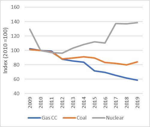
You can also read