Deep learning the Limit Order Book What machines can learn & What can we learn form them? - Tomaso Aste
←
→
Page content transcription
If your browser does not render page correctly, please read the page content below
Milan June 2021

 Deep learning the
 Limit Order Book
 What machines can learn &
 What can we learn form them?

14/06/2021
 Tomaso Aste
 1
9/7/2020 h :// . e ic i k.ac. k/ he e /c / c_ he e/ g . g

 The Financial Computing and Analytics research group
Financial investigates socio- economic systems using methods from
Computing computer science, applied mathematics, computational statistics
 and network theory.
and UCL
Analytics Centre for Blockchain
 Technologies Systemic Risk Centre
Group http://fincomp.cs.ucl.ac.uk/

Silvia Bartolucci Philip Treleaven Guido Germano Fabio CaccioliChristopher ClackGiacomo Livan Paolo Barucca Carolyn Phelan Daniel Hulme Robert E Smith Jiahua Xu
 h :// . e ic i k.ac. k/ he e /c / c_ he e/ g . g

 Tomaso Aste
 1/1

 Research
 •computational finance •empirical finance
 Ariane Chapelle Denise Gorse •data-driven modelling •market microstructure
 Simone Righi Paolo Tasca Geoff Goodell Nikhil Vadgama Jessica James Nick Firoozye
 •artificial intelligence •algorithmic trading
 •financial risk management •high-frequency trading
 Education:
 •blockchain technology •data science
 PhD Doctoral Training Centre in Financial Computing
 •digital economy •big data analytics
 MSc Computational Finance
 •systemic risk •network analysis
 MSc Financial Risk Management
 •numerical pricing of •machine learning
 MSc Financial Technology, forthcoming 2021-22
 derivatives •price formation
 MSc Emerging Digital Technologies, forthcoming 2021-22
 •agent-based simulation •portfolio optimization
 2

What can machines learn?

 3
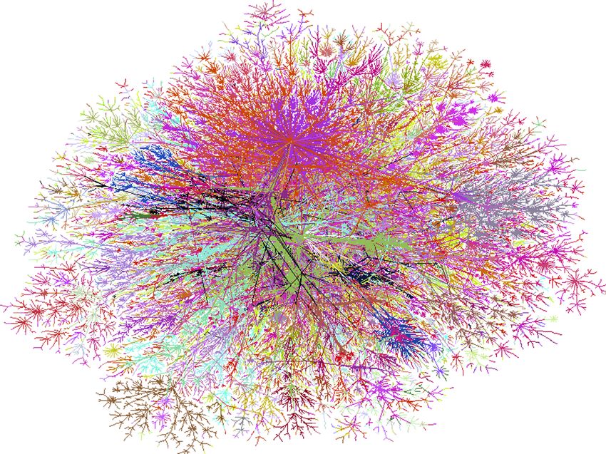
June 2016
 A decade before the "AI winter", going by this NYT article on single layer perceptrons, the AI craze was in May 2016
 full swing. AI and Machine Learning have made some signi cant progress in this last decade, but it's
 always worth remembering how the marketing of AI will always be way ahead of the true capacity of AI.
 While too much undue excitement can hurt a research eld at times, notice that some of the predictions Categories
 about AI agents (recognizing people/faces, language translation) have already become reality today.
 All
 AI

 New York Times 1958 Computer Vision
 Machine Learning

 The perceptron
 Science
 Statistics
 Technology
 User Experience
 Web Performance

 RSS Feed

 (Rosemblatt ‘57, Minsky Papert ‘69)

 www.parvez-ahammad.org/blog/category/ai 1/2

 x1
 w1 x
 1
 x2 w2 x
 2
 f(wx+b) h

 ….
 error function (h)
 wn xn
 f(.) activation function
 xn

 It learns from examples
Frank Rosenblatt with a Mark I
Perceptron computer in 1960 4

forward propagation of signal

x1 w1 x
 1
x2 w2 x2
 f(wx+b) h= f(wx+b)
 h
 ….

 wn xn
 f(.) activation function
xn

x1 Weights are cyclically
 w1 x adjusted in order to minimize
 1
x2 w2 x2 error

 f(wx+b) h error function (h)

 …. wn xn f(.) activation function

xn

 backward propagation of error

Machine learning method

 Prediction
 ….
 Model ….

 Data

 ….
 ….

 ….
 ….
 ….

 ….
 ….

 ….
 …. ….

 Validation
 The circular learning approach where a
 model is automatically learned from
 data through validation and optimization
 is not new
Scientific method vs. machine learning method

 M
 a
 n

 at

 od
 tio

 D

 el
 va

 M
 Selection
 er

 od
 bs

 Parsimony

 el
 O

 Prediction
 Prediction
 • What is novel is the ‘bottom up’ approach that does not need human
 intuition
 The scientific methodfor
 is athe formulation
 circular process: from of the model
 observations (data) we
models that make predictions that are tested against further observations, all
 • Parsimony is no longer central
 he principle of parsimony where simpler models are preferred. The people
 in the• images
 A very large
 are, from number
 the top of models
 right in clockwise order: are automatically
 Nicholas Oresme generated and the
 William of Ockham (1285-1347); Galileo Galilei (1564-1642); Johannes Kepler
 model selection part becomes central
 Isaac Newton (1643-1727). These are philosophers and natural philosophers
What can machines learn?
Machine learning, artificial
intelligence and deep learning had
an enormous success in recent
years
Their successful application has
been mainly in the domain of
image recognition/manipulation
and games

 9

Universal approximation
theorem Cybenko 1989, Hornik 1991

A forward neural network with more than one layer
can approximate any function as far as the network
has a large enough number of neurons
 ….

x h=fNN(x)
 ….

 Reference function
 ….

 Function aproximated by the
 forward neural network
 |fNN(x) – f(x)| <
 10
Recurrent neural networks
are Turing complete
By adding loops (within a layer or backwards) a
recurrent neural network is Turing complete and
therefore it can perform any computation
 …. ….

 h
 x
 ….

 11
Can machines learn markets?

 12
Markets
are gigantic
computation
environments
 Mercati
where machines
and humans
interact to calculate
the price of things
Markets are complex systems
• Markets are complex systems where a large and
 heterogeneous number of variables interact within an
 intricated system of relations
• In markets trades are executed at speeds ranging from
 nanoseconds to years, this are 1015 order of magnitude
 (comparable to our distance to Proxima centaury in
 meters)
• Market variables have statistical properties that are non-
 normal with fat-tails power law distributions
• Markets adapt and change, they are not stationary
Can machines learn markets?
Has a machine that can trade successfully learned
something about the market?

Can we define what does it mean learn in the case of
markets?

A pragmatic perspective:
can machines learn to automate tasks so far
performed by humans?
What can we learn from machines?

 16
Black boxes?

 Bl
 ac
 k
 bo
 x

 Deep learning models return equations or algorithms; these
 are the same kind of outputs of human-made models
 They are however extremely complicated being
 • high-dimensional and
 • non-linear
High dimensionality
High dimensional spaces are very different from the low-
dimensional space we live in.
In particular, the subdivision of high-dimensional spaces into
regions (the basins of optimal solutions) have non-intuitive
properties
• Most of the volume of the region is near the surface
• The number of neighboring regions grows at least exponentially with
 dimension
• The number of interfaces between regions grow combinatorically with
 dimension
• Any ‘gradient descent optimizer’ will be always and unavoidably stuck
 in some saddle-point frontier
 Tomaso Aste and , Denis Weaire, The pursuit of perfect packing. CRC Press, 2008.
 T. Aste, and N. Rivier. "Random cellular froths in spaces of any dimension and curvature." Journal of Physics A: Mathematical and General 28, no. 5 (1995): 1381.
 T Aste, "Dynamical partitions of space in any dimension." Journal of Physics A: Mathematical and General 31, no. 43 (1998): 8577.
Linearity
Linear solutions of linear problems are neat and unique,
they have convenient properties:

1. Small changes in the input produce proportionally small
 changes in the output
2. Small changes in the solution structure or parameters
 also produce small changes in the output
3. Approximate solutions with similar errors are similar

Non-linear solutions are very different
Non-linearity
Non-linear solutions solutions are very different Intriguingly, the way
 deep learning
 systems are trained
 (specifically methods
1. Small changes in the input can produce very such as:
 large changes in the output data sampling, drop
 off, knockout, data
 augmentations, loss
2. Small changes in the solution structure or functions, weight
 parameters can produce very large changes in regularization…)
 seem to overcome
 the output several of these
 issues, at least in
3. Approximate solutions with similar errors can some cases.
 We have a lot of to
 be completely different and there is a learn about how
 these systems
 combinatorial large number of them discover approximate
 solutions
What machines can learn about our complex world -
and what can we learn from them?
They learn approximate solutions that are high-dimensional
and non-linear

The structure of the solution tells us very little about the
model

However, if the learning process if done properly, these
solutions are quite robust and can work also in
circumstances different from the training examples
https://papers.ssrn.com/sol3/papers.cfm?abstract_id=3797711
Deep learning the limit Order Book

 Experiment 1

 A comparative perspective
 https://arxiv.org/pdf/2007.07319.pdf

 22
Jeremy Turiel Antonio Briola

 23
The limit order book (LOB)
 The Limit Order Book (LOB) is a self-organizing system where a
 large number of players interact with offers and bids and
 eventually agree on a transaction price

 10 levels on the sell side
 About 10 transactions
 per second for liquid
 assets on NASDAQ
 10 levels on the buy side

Figure 1: Schematic representation of the LOB structure. It is possible to distinguish between the bid side (left) and
the ask side (right), where both are organised into levels. The first level contains the best bid-price and the best ask- 24
The machine learning system

 Testing with 6 million
 datapoints
 Machine
 INPUT learning OUTPUT
 LOB prices and system Transaction
 volumes for 10 (7 models) price range at
 previous ticks a given
 400-dimesions horizon
 3-dimensions

 Training with 18 million examples
 25
Input
 [(p, v)a0 , (p, v)b0 , (p, v)a1 , (p, v)b1 , ... , (p, v)a10 , (p, v)b10 ],
 20 levels of LOB 10 previous ticks (xt-9,…xt )
pricexlevel and correspondingOverall
 t = 40-dimensions liquidity tuple,of{a,
 a vector b} distinguish ask
 400-dimesions
e best ask and best bid.
 Data:
 NASDAQ, Intel Corp. (INTC) LOB data
 Period:
 training 3 months: 4
 04-02-2019 to 31-05-2019 -> ~ 18 million transactions

 testing 1 month:
 03-06-2019 to 28-06-2019 -> ~ 6 million transactions
 26
1 if x > 0
⇥(x) = (6)
Output 0 if x 0.
4.2 Data preprocessing and labelling
Probability of 3transaction
The data described in Section are preprocessed as follows: after 10, 50 or 100 ticks at a price
within a50,given
{10, 100}. In order toquantile
perform the mappingrange
from continuousestablished from
variables into discrete classes, the following the training set
• The target labels for the prediction task aim to categorise the return at three different time horizons H | ⌧ 2
⌧
quantile levels (0., 0.25, 0.75, 1.) are computed on the returns distribution of the training set and then applied
to the test set. These quantiles are mapped onto classes, denoted with (q 1 , q0 , q+1 ) as reported in Figure 2.
Figure 3 reports the training and test set quantile distributions per horizon H ⌧.
Figure 2: Visual representation of the mapping between quantiles and corresponding classes. Quantiles’ edges (i.e.
(0., 0.25, 0.75, 1.)) define three different intervals. Each specific class (i.e. q 1 , q0 , q+1 ) corresponds to a specific
interval.
• The training set input data (LOB states) are scaled within a (0, 1) interval with the min-max scaling algorithm
Horizons
[34]. The scaler’s training phase is conducted by chunks to optimise the computational effort. The trained
scaler is then applied to the test data. 10, 50, 100 ticks
5
27CNN-LSTM LOB About 60 Layer (type) Output Shape Param # Connected to ===================================================================================== input_1 (InputLayer) [(None, 10, 40)] 0 _________________________________________________________________________________________ reshape (Reshape) (None, 10, 40, 1) 0 input_1[0][0] _________________________________________________________________________________________ thousands conv2d (Conv2D) (None, 10, 20, 16) 48 reshape[0][0] _________________________________________________________________________________________ leaky_re_lu (LeakyReLU) (None, 10, 20, 16) 0 conv2d[0][0] _________________________________________________________________________________________ conv2d_1 (Conv2D) (None, 10, 20, 16) 1040 leaky_re_lu[0][0] _________________________________________________________________________________________ parameters conv2d_2 (Conv2D) (None, 10, 20, 16) 1040 conv2d_1[0][0] _________________________________________________________________________________________ conv2d_3 (Conv2D) (None, 10, 10, 16) 528 conv2d_2[0][0] _________________________________________________________________________________________ leaky_re_lu_1 (LeakyReLU) (None, 10, 10, 16) 0 conv2d_3[0][0] _________________________________________________________________________________________ conv2d_4 (Conv2D) (None, 10, 10, 16) 1040 leaky_re_lu_1[0][0] _________________________________________________________________________________________ conv2d_5 (Conv2D) (None, 10, 10, 16) 1040 conv2d_4[0][0] _________________________________________________________________________________________ conv2d_6 (Conv2D) (None, 10, 1, 16) 2576 conv2d_5[0][0] _________________________________________________________________________________________ leaky_re_lu_2 (LeakyReLU) (None, 10, 1, 16) 0 conv2d_6[0][0] _________________________________________________________________________________________ conv2d_7 (Conv2D) (None, 10, 1, 16) 1040 leaky_re_lu_2[0][0] _________________________________________________________________________________________ conv2d_8 (Conv2D) (None, 10, 1, 16) 1040 conv2d_7[0][0] _________________________________________________________________________________________ conv2d_9 (Conv2D) (None, 10, 1, 32) 544 conv2d_8[0][0] _________________________________________________________________________________________ conv2d_11 (Conv2D) (None, 10, 1, 32) 544 conv2d_8[0][0] _________________________________________________________________________________________ leaky_re_lu_3 (LeakyReLU) (None, 10, 1, 32) 0 conv2d_9[0][0] _________________________________________________________________________________________ leaky_re_lu_5 (LeakyReLU) (None, 10, 1, 32) 0 conv2d_11[0][0] _________________________________________________________________________________________ max_pooling2d (MaxPooling2D) (None, 10, 1, 16) 0 conv2d_8[0][0] _________________________________________________________________________________________ conv2d_10 (Conv2D) (None, 10, 1, 32) 3104 leaky_re_lu_3[0][0] _________________________________________________________________________________________ conv2d_12 (Conv2D) (None, 10, 1, 32) 5152 leaky_re_lu_5[0][0] _________________________________________________________________________________________ conv2d_13 (Conv2D) (None, 10, 1, 32) 544 max_pooling2d[0][0] _________________________________________________________________________________________ leaky_re_lu_4 (LeakyReLU) (None, 10, 1, 32) 0 conv2d_10[0][0] _________________________________________________________________________________________ leaky_re_lu_6 (LeakyReLU) (None, 10, 1, 32) 0 conv2d_12[0][0] _________________________________________________________________________________________ leaky_re_lu_7 (LeakyReLU) (None, 10, 1, 32) 0 conv2d_13[0][0] _________________________________________________________________________________________ concatenate (Concatenate) (None, 10, 1, 96) 0 leaky_re_lu_4[0][0] leaky_re_lu_6[0][0] leaky_re_lu_7[0][0] _________________________________________________________________________________________ reshape_1 (Reshape) (None, 10, 96) 0 concatenate[0][0] _________________________________________________________________________________________ lstm (LSTM) (None, 64) 41216 reshape_1[0][0] _________________________________________________________________________________________ dense (Dense) (None, 3) 195 lstm[0][0] Z. Zhang, S. Zohren, and S. Roberts. ===================================================================================== Total params: 60,691 “DeepLOB: Deep Convolutional Trainable params: 60,691 Non-trainable params: 0 Neural Networks for Limit Order _________________________________________________________________________________________ Books”. In: IEEE Transactions on Signal Processing 67.11 (June 2019), pp. 3001–3012 Quantile probability 28
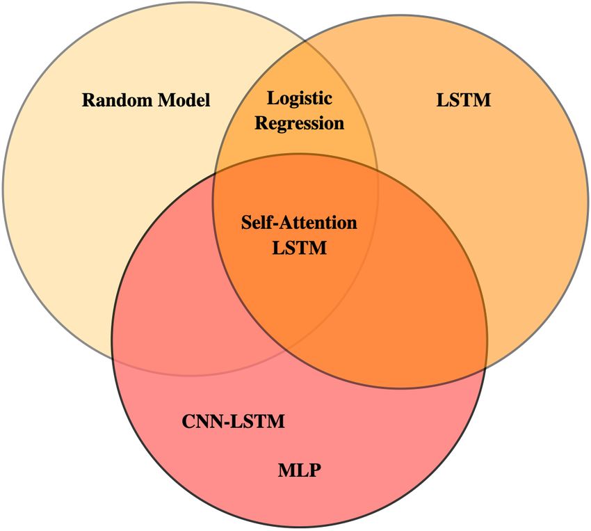
Models
Can a Multilayer Perceptron learn the LOB efficiently?
And how will it do with respect to other simpler and more
complicated models?

We investigate and compare 7 different models with increasing
levels of complexity
1. Random Model – uniform probability outcome prediction
2. Naive Model – output most represented in training
3. Logistic Regression – simple perceptron
4. Multilayer Perceptron – deep learning model
5. Shallow LSTM – deep learning with memory
6. Self-Attention LSTM – deep learning with memory & loop
7. CNN-LSTM – state of the art deep learning
 29
Multilayer perceptron
 LOB Over 2 million
 parameters

 ….

 ….

 ….
 ….

 ….

 ….
 x
 q

 ….
 ….

 ….
 ….

 ….

 ….
 400 515 1024 1024 512 64 3
 Layer (type) Output Shape Param #
 =================================================================
 input_1 (InputLayer) [(None, 10, 40)] 0
 _________________________________________________________________
 flatten (Flatten) (None, 400) 0
 _________________________________________________________________
 dense (Dense) (None, 400) 160400
 _________________________________________________________________
 dense_1 (Dense) (None, 512) 205312
 _________________________________________________________________
 dense_2 (Dense) (None, 1024) 525312
 _________________________________________________________________
 dense_3 (Dense) (None, 1024) 1049600
 _________________________________________________________________

 Quantile probability
 dense_4 (Dense) (None, 64) 65600
 _________________________________________________________________
 dense_5 (Dense) (None, 3) 195
 =================================================================
 Total params: 2,006,419. Trainable params: 2,006,419, Non-trainable params: 0
 _________________________________________________________________
 30
Logistic regression

 x0
 0
 x1 1 P
 e i i xi
 p= P
 …. 1 + e i i xi
 n ⇣ ⇤ 1
 ⌘ X ⇣ 1⌘ X ⇣ 1⌘
 ˆ
 ⌃ = ˆ
 ⌃ ˆ
 ⌃
 c s
 xn ~400 parameters
 i,j
 c2C
 i,j
 s2S
 i,j

 Y
 Pc (Xc )
 c2C
 P (X) = Y
One-layer perceptron (x0=1) Ps (Xs )
 31
Shallow LSTM
 About 5
 LOB
 thousands
 parameters

 x
 q

 ….

 ….
 400 20 3
 Model: "model"
 _________________________________________________________________
 Layer (type) Output Shape Param #
 =================================================================
 input_1 (InputLayer) [(None, 10, 40)] 0

 Quantile probability
 _________________________________________________________________
 lstm (LSTM) (None, 20) 4880
 _________________________________________________________________
 dense (Dense) (None, 3) 63
 =================================================================
 Total params: 4,943
 Trainable params: 4,943
 Non-trainable params: 0
 _________________________________________________________________

 32
Self-Attention LSTM –
 LOB

 About 25
 thousands
 parameters
 __________________________________________________________________________________________________
 Layer (type) Output Shape Param # Connected to
 ==================================================================================================
 input_1 (InputLayer) [(None, 10, 40)] 0
 __________________________________________________________________________________________________
 lstm (LSTM) (None, 10, 40) 12960 input_1[0][0]
 __________________________________________________________________________________________________
 attention_score_vec (Dense) (None, 10, 40) 1600 lstm[0][0]
 __________________________________________________________________________________________________
 last_hidden_state (Lambda) (None, 40) 0 lstm[0][0]
 __________________________________________________________________________________________________
 attention_score (Dot) (None, 10) 0 attention_score_vec[0][0]
 last_hidden_state[0][0]
 __________________________________________________________________________________________________
 attention_weight (Activation) (None, 10) 0 attention_score[0][0]
 __________________________________________________________________________________________________
 context_vector (Dot) (None, 40) 0 lstm[0][0]
 attention_weight[0][0]
 __________________________________________________________________________________________________
 attention_output (Concatenate) (None, 80) 0 context_vector[0][0]
 last_hidden_state[0][0]
 __________________________________________________________________________________________________
 attention_vector (Dense) (None, 128) 10240 attention_output[0][0]
 __________________________________________________________________________________________________
 dense (Dense) (None, 3) 387 attention_vector[0][0]
 ==================================================================================================
 Total params: 25,187
 Trainable params: 25,187
 Non-trainable params: 0

 Quantile probability
 __________________________________________________________________________________________________

 33
Model Details
The models range a parameter space dimension from zero
to one million
 Number of Number of Learning Training
 Model Input
 layers (⇤) parameters(⇤⇤) rate epochs
 Random - 0 0 -
 Naive LOB 1 1 -
 Logistic Reg. LOB 2 4 ⇥ 102 10 3
 30
 MLP LOB 7 2.0 ⇥ 106 10 3
 30
 Shallow LSTM LOB 3 4.9 ⇥ 103 10 3
 30
 Self-Attention LSTM LOB 4 2.5 ⇥ 104 10 3
 30
 CNN-LSTM LOB 28 6.0 ⇥ 104 10 3
 30

 Table 1: Summary of the inputs and hyperparameters used in the models in this
 article. (⇤) The number of layers includes the input and the output layer. (⇤⇤) The
 number of parameters is approximated to the nearest order of magnitude and
 truncated for readability.

 34
Performance metrics

We tested performances of the prediction for each
of the quantile regions by computing:
Precision, Recall and F-measure
In order to correct for class imbalance we also tested:
balanced Accuracy, weighted Precision, weighted
Recall and weighted F-score

Furthermore, two multi-class correlation metrics between
forecasted and real labels computed:
Matthews Correlation Coefficient (MCC) and Cohen’s Kappa

 35
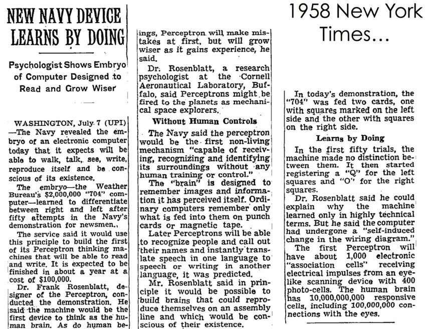
Results
Table 7: Performance metrics for horizons H ⌧ computed on the test folds. The column labels H10, H50, H100 refer
to HPerformances at three horizons: 10, 50, 100 ticks
 ⌧ | ⌧ = 10, H ⌧ | ⌧ = 50, H ⌧ | ⌧ = 100, respectively.

 Random Model Naive Model Logistic Regression Shallow LSTM Self-Attention LSTM CNN-LSTM Multilayer Perceptron
 H10 H50 H100 H10 H50 H100 H10 H50 H100 H10 H50 H100 H10 H50 H100 H10 H50 H100 H10 H50 H100
 Balanced Accuracy 0.33 0.33 0.33 0.33 0.33 0.33 0.46 0.47 0.53 0.47 0.51 0.38 0.55 0.42 0.52 0.57 0.56 0.55 0.56 0.59 0.61
 Weighted Precision 0.41 0.41 0.41 0.16 0.30 0.30 0.54 0.56 0.62 0.58 0.57 0.65 0.61 0.50 0.47 0.62 0.61 0.61 0.62 0.62 0.63
 Weighted Recall 0.33 0.33 0.33 0.40 0.55 0.54 0.59 0.59 0.61 0.58 0.58 0.57 0.61 0.45 0.34 0.62 0.62 0.62 0.62 0.63 0.63
 Weighted F-Measure 0.34 0.35 0.35 0.23 0.40 0.39 0.53 0.53 0.60 0.51 0.57 0.47 0.60 0.40 0.24 0.62 0.61 0.61 0.61 0.62 0.63
 Precision quantile [0, 0.25] 0.26 0.26 0.26 0 0 0 0.57 0.57 0.57 0.57 0.56 0.58 0.60 0.37 0.55 0.59 0.59 0.59 0.59 0.59 0.59
Precision quantile [0.25, 0.75] 0.55 0.55 0.55 0.40 0.55 0.54 0.59 0.60 0.63 0.59 0.62 0.56 0.62 0.55 0.52 0.65 0.64 0.63 0.64 0.66 0.67
 Precision quantile [0.75, 1] 0.20 0.20 0.20 0 0 0 0.31 0.38 0.58 0.57 0.43 0.97 0.57 0.52 0.26 0.57 0.57 0.57 0.59 0.58 0.57
 Recall quantile [0, 0.25] 0.33 0.33 0.33 0 0 0 0.55 0.59 0.59 0.06 0.62 0.22 0.35 0.81 0.62 0.54 0.55 0.53 0.60 0.59 0.60
 Recall quantile [0.25, 0.75] 0.33 0.33 0.33 1 1 1 0.82 0.81 0.76 0.85 0.69 0.93 0.76 0.44 0.01 0.71 0.72 0.74 0.74 0.70 0.68
 Recall quantile [0.75, 1] 0.33 0.33 0.33 0 0 0 0 0 0.23 0.51 0.23 0 0.53 0.004 0.92 0.46 0.42 0.39 0.34 0.46 0.54
 F-Measure quantile [0, 0.25] 0.29 0.29 0.29 0 0 0 0.56 0.57 0.58 0.11 0.59 0.31 0.44 0.503 0.58 0.57 0.57 0.56 0.59 0.59 0.59
F-Measure quantile [0.25, 0.75] 0.42 0.42 0.42 0.57 0.71 0.70 0.70 0.70 0.68 0.69 0.65 0.70 0.68 0.489 0.02 0.68 0.68 0.68 0.69 0.68 0.67
 F-Measure quantile [0.75, 1] 0.25 0.25 0.25 0 0 0 0 0 0.33 0.54 0.30 0 0.55 0.009 0.40 0.51 0.48 0.46 0.43 0.51 0.56
 MCC 0 0 0 0 0 0 0.24 0.25 0.30 0.23 0.27 0.14 0.31 0.120 0.25 0.34 0.34 0.32 0.34 0.36 0.38
 Cohen’s Kappa 0 0 0 0 0 0 0.21 0.22 0.30 0.20 0.27 0.10 0.30 0.105 0.16 0.34 0.33 0.32 0.33 0.36 0.38

6 Discussion
 36
considerations, one expects to obtain analogous results to the presented Bayesian test. Future work shall include
Results
additional tests.

 37
H ⌧| ⌧ = 10 H ⌧| ⌧ = 50 H ⌧| ⌧ = 100
Ranking representation of results from Multilayer
 Multilayer Perceptron the Bayesian correlated t-testMultilayer
 Perceptron [4] based on the MCC performance
 Perceptron
 Results
odels on the same
 CNN -line
 LSTMindicate statistical equivalence
 CNN - LSTMand models in lower CNN rows perform worse (statistically
 - LSTM
 ) than the ones in the upper rows. Shallow LSTM
 Self-Attention
 Bayesian LSTM t-test from MCC measure Multinomial Logistic Regression
 correlated
 H ⌧ | ⌧LSTM= 10
 Multinomial Logistic Regression
 H ⌧ | ⌧ = 50 H ⌧ | ⌧ = 100
 • Multilayer perceptron is
 Shallow
 Multinomial Logistic
 Multilayer Regression
 Perceptron
 Self-Attention LSTM
 Multilayer Perceptron
 Self-Attention LSTM
 Multilayer Perceptron the best performing
 CNN - LSTM
 Naive Model CNN
 Naive-Model
 LSTM CNN - LSTM
 Random Model Random Model
 Shallow LSTM
 Shallow LSTM • CNN-LSTM is second-
 Self-Attention LSTM Multinomial Logistic Regression

 Shallow LSTM
 Multinomial Logistic Regression Random Model best with comparable
 Multinomial Logistic Regression
 Self-Attention LSTM Self-Attention LSTM
 performances
 Naive Model Naive Model
 Random Model
 anking representation Random Model
 of results from the Bayesian
 Shallow LSTM • Logistic regression has
 correlated t-test [4] based on the F-measure performance
 odels on the same line indicate statistical equivalence and models in lower perform worse (statisticallygood performances
 rowsModel
 Random
 ) than the ones in the upper rows.
 Bayesian correlated t-test from F measure comparable with LSTM
 H | ⌧ = 10 H | ⌧ = 50 H | ⌧ = 100
 based on the F-measure performanceand self-attention LSTM
 ⌧ ⌧ ⌧
Ranking representation of results
 Multilayer Perceptron from the Bayesian correlated t-test [4]
 odels on the same Multilayer Perceptron
 CNN -line indicate statistical equivalence and models in lower rows perform worse (statistically
 LSTM
 ) than the Self-Attention
 ones in the upper
 LSTM rows.
 CNN - LSTM
 Multilayer Perceptron
 • Naïve and Random are
 Shallow LSTM
 Multinomial Logistic Regression
 Shallow LSTM
 CNN - LSTM
 Multinomial Logistic Regression
 worst
 H ⌧ | ⌧ = 10 H ⌧ | ⌧ = 50 H ⌧ | ⌧ = 100
 Naive Model
 Multilayer Perceptron Multinomial Logistic Regression Shallow LSTM
 Multilayer Perceptron
 RandomLSTM
 CNN - Model Self-Attention
 CNN - LSTM LSTM Multilayer Perceptron
 Self-Attention LSTM
 Self-Attention LSTM
 Naive Model Naive Model
 Shallow LSTM CNN - LSTM
 Multinomial Logistic Regression Random LSTM
 Shallow Model Random
 Multinomial Model
 Logistic Regression
 Naive Model Multinomial Logistic Regression Shallow LSTM
 38
ased model clustering
 Results
 One can attempt to
 cluster the models
 together based on their
 Naive
 performances

 One can note that
 memory/recurrent loops
 (LSTM) play little role in
 performances. Most of
 the information is
 processed forwards from
 the LOB input
Deep learning the limit Order Book

 Experiment 2

 Reinforcement Learning
 https://arxiv.org/abs/2101.07107

 40
Reward
 Testing with 6 million
 examples
INPUT
LOB prices and Reinforcement
volumes for 10 learning
 algorithm
 OUTPUT
previous ticks Action:
400-dimesions 1. Sell,
 2. stay,
 3. buy,
 4. stop_loss
 41

 Training with ~6 millions
 selected examples
Deep reinforcement learning: architecture
 Profits of the ‘agent’ depending on the action

The algorithm buys Q-learning Q sell stay buy Stop_loss

or sells or holds
 approach neutral
 wa rd
 Long
 Re
one unit of Intel short

Corporation stock Gaussian process regressor

(INTC) on
NASDAQ during Sell

 ….
 ….
the month of June x stay
 Buy

 ….
2019

 ….
 stop_loss

 ….
It is trained during
the previous 3 4002 +3 64 64 4

months About 30,000 parameters
 42
Deep reinforcement learning: training
 Profits of the ‘agent’ depending on the action
 Q sell stay buy Stop_loss
We train on 25 selected neutral
 a rd
significant events containing Long
 Re w
 short
about 250,000 ticks
 Gaussian process regressor

• Training on 60 days Sell

 ….
 ….
 04/02/2019-30/04/2019 x stay
• Validation on 22 days Buy

 ….

 ….
 stop_loss

 ….
 01/05/2019-31/05/2019
• Testing on 20 days
 03/06/2019-28/06/2019 4002 +3 64 64 4

 About 30,000 parameters
 43
Deep reinforcement learning: input
 Profits of the ‘agent’ depending on the action
We test for three sets of Q sell stay buy Stop_loss
input information; all neutral
 rd
 wa
have the full LOB (400 Long
 Re
 short
dimension) plus:
 Gaussian process regressor

1. State of the agent
2. State of the agent & Sell

 ….
 ….
 market price minus price x stay
 Buy
 paid for the unit (mark to

 ….

 ….
 stop_loss

 ….
 market profit)
3. State of the agent & price
 paid for the unit (mark to 4002 +3 64 64 4

 market) & bid-ask spread About 30,000 parameters
Deep reinforcement learning: performances
 1. LOB + 2. LOB + 3. LOB +
 State of the
 (a)
 agent State of the(b) agent & State of (c)the agent & price paid
 Fig. 2. Cumulative mean return across the 30 ensemble elements (a), daily mean cumulative return and standard deviation (b) and trade return distribution
 price. paid (a)for the unit
 (c) for the full test (20 days) and agent state definition S c201 for the unit (b)
 (a)
 (mark to market) & (c)(b
 (mark
 Fig. 2. Cumulativeto meanmarket)
 return across the 30 ensemble
 (c) for the full test (20 days) and agent state definition
 bid-ask
 Fig. 3.elements
 Cumulative meanspread
 (a), daily mean
 returncumulative
 across thereturn and standard
 30 ensemble
 S the. full test (20 days) and agent state definition S
 deviation
 elements (b) m
 (a), daily a
 (c) for c201 . c202

 ⇥103 ⇥105 ⇥103
 1.0
 Cumulative P&L ($)

 Cumulative P&L ($)

 Cumulative P&L ($)
 8 6

 6 4
 0.5
 4
 2
 0.0 2
 (b)(a) 0 (c)
 (b) 0 (c)
 0 2 4 6 0 1 2 3 4 5 6 0 1 2 3 4 5
n across the 30 ensemble elements (a),
 Tickdaily
 meanmean cumulative return
 6
 Fig. 3. Cumulative time return
 (LOB updates) and standard
 across the 30 ensemble deviation
 elements⇥10
 Tick (b)
 (a), daily
 time and
 mean
 (LOBtrade return distribution
 cumulative
 updates) return
 ⇥106 and standard deviation (b) and
 Tick time (LOBtrade return distribution
 updates) ⇥106
nd agent state definition
 (c) S
 for the. full test (20 days) and agent state definition Sc202 .
 c201
 (a) (b)(a) (c)(b)
 (a) (c)
 (b
 Fig. 2. Cumulative mean return across the 30 ensemble elements
 Fig. 3. (a), daily
 Cumulative meanmean cumulative
 return across thereturn and standard
 30 ensemble
 Fig. 2 deviation
 4.elements (b) and
 (a), daily
 Cumulative
 10 mean meantrade
 return returnthe
 cumulative
 across distribution
 return and standard
 30 ensemble deviation
 elements (b) m
 (a), daily a
 3
 (c) for the full test (20 days) and agent state definition . full test (20 days) and agent state definition
 10
 Number of trades

 (c) S
 Number of trades

 Number of trades
 for the
 c201 (c) for the. full test (20 days) and agent state definition S
 Sc202 . c203
 101
 102
 101
 VI. C ONCLUSIONS
 101

 100 In the0 present work we showed how to to successfully train
 100 10
 3000 2000 1000 0 1000 2000 3000 4000
 2000 0 2000 4000 6000 and deploy4000DRL2000 models
 0 2000 in
 4000the6000context
 8000 of high frequency
 Trade Profit ($)
 Trade Profit ($) trading. We investigate how($three
 Trade Profit ) different state definitions
 (c) affect the out-of-sample performance of the agents and we
 (b)(a) (b)
 (c) (c)
an cumulative return and standard deviation (b) and trade return distribution
 find that the knowledge of the mark-to-market return of their
 Fig. 4.
n across the 30 ensemble Cumulative
 elements meanmean
 (a), daily return across thereturn
 cumulative 30 ensemble elements
 and standard (a), daily
 deviation mean
 (b) and cumulative
 trade returncurrent position
 and standard
 return distribution is highly
 deviation beneficial
 (b) and trade both for the global P&L
 return distribution
 (c) S
nd agent state definition for the. full test (20 days) and agent state definition Sc203 .
 c202 function and for the single trade reward. However, it should be
 (a) (b)(a) (c)(b) (c)
 noticed that, independently on the state definition, the agents
Deep reinforcement learning: performances

What the agent learned?

• The agent increases profits by about 100 folds by
 trading 10 to 100 times more often using information
 about the reference unit price (mark to market). The
 agent learns to increase profits while increasing trading
 frequency despite the bid-ask spread cost
• Risk is reduced considerably
• The extra information on the bid-ask spread does not
 increase performances
Conclusions
• Artificial intelligence is providing increasingly powerful
 new instruments
• It is almost a surprise that a complicated self-trained
 machine, such as the Multi Layer Perception, can learn
 something about the price formation mechanism on the
 LOB
• It is almost a surprise that a self-learning agent can
 discover trading strategies
• Results are very good but not ground-breaking. Are we
 at the beginning or at the end of this journey?
Links and
references
LINKS

FCA Group Page:
http://fincomp.cs.ucl.ac.uk/introd
 RELEVANT PAPERS
uction/

 Aste, Tomaso. "What machines can learn about our complex world-and what can we learn
My articles: from them?." Available at SSRN 3797711 (2021).
https://scholar.google.co.uk/citati Briola, Antonio, Jeremy Turiel, Riccardo Marcaccioli, and Tomaso Aste. "Deep
ons?user=27pUbTUAAAAJ&hl=e Reinforcement Learning for Active High Frequency Trading." arXiv preprint
n arXiv:2101.07107 (2021).
Software: Briola, Antonio, Jeremy Turiel, and Tomaso Aste. "Deep Learning Modeling of the Limit
TMFG & Clique Forests Order Book: A Comparative Perspective." Available at SSRN 3714230 (2020).
https://github.com/cvborkulo/Net
workComparisonTest/pull/5
https://uk.mathworks.com/matlab
central/fileexchange/56444-tmfg

 48
You can also read