Data-driven flood emulation: Speeding up urban flood predictions by deep convolutional neural networks
←
→
Page content transcription
If your browser does not render page correctly, please read the page content below
Received: 28 April 2020     Revised: 3 October 2020     Accepted: 18 November 2020
DOI: 10.1111/jfr3.12684

ORIGINAL ARTICLE

Data-driven flood emulation: Speeding up urban flood
predictions by deep convolutional neural networks

Zifeng Guo1                  |    Joa~o P. Leita~o2             | Nuno E. Simões3 |                          Vahid Moosavi1

1
 Chair of Digital Architectonics, Institute
of Technology in Architecture (ITA),
                                                      Abstract
Department of Architecture, Swiss Federal             Computational complexity has been the bottleneck for applying physically
Institute of Technology Zurich (ETHZ),
                                                      based simulations in large urban areas with high spatial resolution for efficient
Zürich, Switzerland
2                                                     and systematic flooding analyses and risk assessment. To overcome the issue
 Department of Urban Water
Management, Swiss Federal Institute of                of long computational time and accelerate the prediction process, this paper
Aquatic Science and Technology (Eawag),               proposes that the prediction of maximum water depth can be considered an
Dübendorf, Switzerland
3
                                                      image-to-image translation problem in which water depth rasters are gener-
 INESC Coimbra, Department of Civil
Engineering, University of Coimbra,                   ated using the information learned from data instead of by conducting simula-
Coimbra, Portugal                                     tions. The proposed data-driven urban pluvial flood approach is based on a
                                                      deep convolutional neural network trained using flood simulation data
Correspondence
Zifeng Guo, Chair of Digital                          obtained from three catchments and 18 hyetographs. Multiple tests to assess
Architectonics, Institute of Technology in            the accuracy and validity of the proposed approach were conducted with both
Architecture (ITA), Department of
                                                      design and real hyetographs. The results show that flood prediction based on
Architecture, Swiss Federal Institute of
Technology Zurich (ETHZ), Stefano-                    neural networks use only 0.5% of the time compared with that of physically
Franscini-Platz 1, Zürich, 8093,                      based models, with promising accuracy and generalizability. The proposed
Switzerland.
Email: guo@arch.ethz.ch
                                                      neural network can also potentially be applied to different but relevant prob-
                                                      lems, including flood analysis for flood-safe urban layout planning.

                                                      KEYWORDS
                                                      convolutional neural network, data-driven emulation, fast water depth prediction, flood
                                                      modelling

1 | INTRODUCTION                                                                     possible to inform citizens of likely urban pluvial flooding
                                                                                     in advance, so that precautionary measures can be taken.
The combination of rapid urbanization and the rainfall
intensity increase due to climate change is posing great
challenges for flood risk management (Plate, 2002). Fast                             1.1 | Rapid flood modelling
flood prediction methods are required to conduct system-
atic analyses and investigations of different urban plan-                            The current bottleneck for rapid urban pluvial flood ana-
ning and climate change scenarios (Zheng, Thibaud,                                   lyses is the long computational time required by physi-
Leonard, & Westra, 2015). Furthermore, if rapid urban                                cally based simulation models. The problem becomes
pluvial flood predictors are integrated with high temporal                           extremely significant for large simulation areas with high
resolution online rainfall forecast services, it will be                             spatial resolutions (small raster grid size). Solutions for
This is an open access article under the terms of the Creative Commons Attribution-NonCommercial License, which permits use, distribution and reproduction in any
medium, provided the original work is properly cited and is not used for commercial purposes.
© 2020 The Authors. Journal of Flood Risk Management published by Chartered Institution of Water and Environmental Management and John Wiley & Sons Ltd.

J Flood Risk Management. 2021;14:e12684.                                                                            wileyonlinelibrary.com/journal/jfr3       1 of 14
https://doi.org/10.1111/jfr3.12684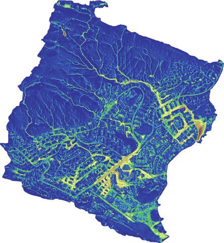
2 of 14                                                                                                              GUO ET AL.

solving this issue have been previously identified, which       computer graphics. For example, regression forest was
include reducing the dimensionality of flood representa-        used to learn the dynamic process of particle-based simu-
tion (e.g., Samuels, 1990) or neglecting the inertial and       lations for real-time animation and layout planning
advection terms of the momentum equation (e.g., Bates,          (Feng, Yu, Yeung, Yin, & Zhou, 2016; Ladický, Jeong,
Horritt, & Fewtrell, 2010; Bradbrook, Lane, Waller, &           Solenthaler, Pollefeys, & Gross, 2015). Later, a fully-
Bates, 2004; Chen, Djordjevic, Leandro, & Savic, 2007).         connected neural network was proposed by Mustafa
However, according to Teng et al. (2017), physically            et al. (2018) for flood-driven urban planning. However,
based models are still not suitable for areas larger than       the approach had a main drawback that the training data
1,000 km2 with a raster grid size smaller than 10 m. In         for the neural network was the input parameters of a ter-
urban areas, the required raster grid size should be            rain generator rather than raw elevation data, and conse-
between 1 m and 5 m to capture the urban features               quently the results cannot be extended to other scenarios.
(Fewtrell, Bates, Horritt, & Hunter, 2008; Leit~ao, Boonya-     Recently, this issue was handled by introducing a prior
Aroonnet, Prodanovic, & Maksimovic, 2009).                    terrain feature extraction process (e.g., Leit~ao, Zaghloul, &
    Non-physically based models, on the other hand, are         Moosavi, 2018; Zaghloul, 2017).
based on simplified hydrological concepts such as topo-             Using artificial neural networks (or neural networks)
graphic depressions (L'homme et al., 2008) or the transi-       for flood prediction and susceptibility mapping has
tion rules of cellular automata (e.g., Ghimire et al., 2013;    recently become more frequent due to (a) neural net-
Guidolin et al., 2016). These methods can be                    works were shown to be able to approximate any strong
implemented using parallel computing techniques to sig-         non-linear correlation and (b) recurrent neural networks
nificantly improve the computational speed. Recently,           (Schuster & Paliwal, 1997), a neural network structure
Jamali, Bach, Cunningham, and Deletic (2019) have               which stacks multiple layers dynamically, were found
shown that the cellular automata models can predict             effective for processing time series data. Recurrent neural
maximum water depths of large urban areas in a few              networks were used to forecast long-term water level for
minutes. But the main drawback lies in its sensitivity to       individual locations from corresponding inputs of rainfall
simulation time steps and raster grid size. Reducing the        intensity (e.g., Chang, Chen, Lu, Huang, & Chang, 2014;
time step or grid size still causes a significant increase in   Gude, Corns, & Long, 2020), or combined with self-
simulation time. Non-physically based approaches have           organizing maps to estimate maximum water depths
become significantly faster than physically based               (Kim & Han, 2020a). Fully-connected neural networks
approaches, however, they are still considered not fast         were used to estimate water levels and flow velocities at
enough for applications that require a considerable num-        specific coordinates based on statistical and topographical
ber of simulations, such as flood-driven optimizations          inputs such as slope, aspect and curvatures (e.g., Bui
and planning. Also, it is known that the computational          et al., 2020; Kim & Han, 2020b). However, a main draw-
time is non-linearly related with the raster resolutions.       back of fully-connected neural networks is the exponen-
Doubling the resolution may cause ten times more simu-          tial growth of parameters on large inputs (LeCun,
lation times (Guidolin et al., 2016).                           Bengio, & Hinton, 2015), which cause significant chal-
                                                                lenges when trying to utilize spatial information from
                                                                adjacent pixels (raster cells) for two-dimensional simula-
1.2 | Data-driven methods for flow and                          tions. A workaround of this problem was shown by
flood related problems                                          Berkhahn, Fuchs, and Neuweiler (2019) through a com-
                                                                bination of pruning zero-cells from the neural network
Recently, solving physics-related problems with machine         inputs and using multiple small neural networks that are
learning techniques has become a research field receiving       responsible for different local areas instead of one large
growing attention due to its computational efficiency and       network that predicts the entire catchment area.
the ability to learn and generalize from data
(e.g., Greydanus, Dzamba, & Yosinski, 2019). This direc-
tion is also called “surrogate modelling” because the           1.3 | Data-driven flow and flood
machine learning models act as the “surrogate” of the           modelling using convolutional neural
physically based simulations hypothesising that the             networks
models will learn the target system regardless of the
actual physical process if sufficient data are provided.        Despite the variety of available algorithms, convolutional
Making surrogate models for flow and flood related prob-        neural networks (CNNs) in particular, have received
lems has been investigated using different methods. The         strong attention due to their ability to (a) process raw
noticeable early attempts can be found from the field of        data in image format and (b) utilize spatial information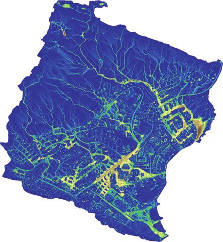
GUO ET AL.                                                                                                          3 of 14

from adjacent pixels with many fewer parameters com-          2 | PROB LEM STATEM ENT
pared to other type of neural networks. Beyond its origi-
nal goal for image classification and object detections in    The above review has suggested that data-driven methods
computer graphics, CNNs have been used to solve flow-         are promising for addressing physics-related problems,
related problems in a way that the boundary conditions        including urban pluvial flood prediction. However, most
were discretized into images (rasters) with multiple          previous flood-related studies using artificial neural net-
image channels. For example, the velocity and pressure        works did not utilize the spatial information of catch-
fields of steady inlet air flow around objects of interest    ment areas. Among the few existing studies, CNNs were
were inferred by CNNs from discretized inputs (e.g., Guo,     used for classifications (e.g., flood susceptibility mapping
Li, & Iorio, 2016; Thuerey, Weißenow, Prantl, &               and flood extent mapping) rather than numerical predic-
Hu, 2020; Tompson, Schlachter, Sprechmann, &                  tions. Therefore, we propose to use CNNs for rapid data-
Perlin, 2017). Chu and Thuerey (2017) used weight-            driven flood predictions, specifically, to predict the maxi-
sharing CNNs (multiple CNN instances sharing the same         mum water depth from the inputs of both elevation ras-
trainable parameters) to learn the feature descriptor of      ters and hyetographs. Our main contributions include
smoke flows for synthesizing high-resolution predictions      (a) investigating CNNs as an end-to-end method for flood
from low-resolution simulations. Hennigh (2017)               predictions, which means the model directly predicts the
predicted the flow dynamics by decoding the compressed        water depth values from the raw inputs; (b) introducing a
initial conditions through a series of weight-sharing         CNN architecture that combines both spatial inputs (ras-
CNNs that stack on after each other. Gao, Sun, and            ters) and vector inputs (hyetographs); and (c) providing a
Wang (2020) used CNNs for handling inputs with irregu-        systematic pipeline that can potentially be used to
lar boundaries using elliptic coordinate transformations.     address other relevant problems.
    The use of CNNs for flood-related problems, espe-             Our study currently focuses on the prediction of maxi-
cially for urban pluvial flood predictions, has not           mum water depth and neglects the temporal dynamic of
received much attention. This may be justified by, first,     flooding. The maximum water depth reflects the worst
in contrast to the fluid dynamic experiments focusing on      flooding cases and is critical for urban planning, risk
objects that can be rasterized to a relatively low resolu-    management, and damage assessment (Jamali
tion without significant information loss (e.g., 256 × 256    et al., 2018). The prediction of maximum water depth can
pixels), flood prediction is usually conducted in large       be further divided into three cases: (a) different storms in
catchment areas that require sufficient spatial resolution    the same catchment; (b) same storm in different catch-
to be preserved. Therefore, building the CNNs for flood       ments, and (c) considering both the rainfall and catch-
prediction typically require large input sizes and thus       ment variations. As a first step, we would focus on the
more layers, creating difficulties in the training step of    first case and investigate the ability of generalization of
CNNs. Second, for the purpose of flood prediction, train-     CNNs on different rainfall inputs in specific catchments.
ing CNNs requires a large dataset in raster format. Con-      The present work does not include flow velocity, but
sidering the scale and spatial and temporal resolutions of    other studies have shown that it can be done by adding
typical flood simulation tasks, it is computationally and     extra image channels to the output, and the predictions
memory expensive to prepare a large dataset. Lacking          between different image channels are independent
proper datasets has been the main obstacle for data-          (e.g., Hennigh, 2017; Thuerey et al., 2020).
driven flood modelling and prediction studies. Neverthe-
less, a few recent studies have shown that CNNs are
promising for solving flood-related problems with             3 | P R O P O S E D A PP R O A C H
corresponding data available. For example, CNNs can be
effective for flood extent mapping using aerial or street     3.1 | Framework
view imagery (e.g., Gebrehiwot, Hashemi-Beni, Thomp-
son, Kordjamshidi, & Langan, 2019; Moy de Vitry,              Our urban pluvial flooding approach proposes a CNN
Kramer, Wegner, & Leit~ao, 2019). These methods can           model as the main prediction mechanism. The key idea
potentially be used to replace physically based simulators    is that the flood prediction task can be regarded as an
for massive data collection. Wang, Fang, Hong, and            image-to-image translation problem where both the input
Peng (2020) adopted CNNs for flood susceptibility map-        and output are images (rasters) of different data. The pro-
ping from multiple topographic features that are derived      posed CNN model operates on the patches rather than
from the raw elevation data. Based on the input informa-      the entire catchment area. The reasons for working with
tion, the model predicts the flood sensitivity as five out-   patches includes: (a) patches from different locations
put categories.                                               may share similarities that help the CNN learn and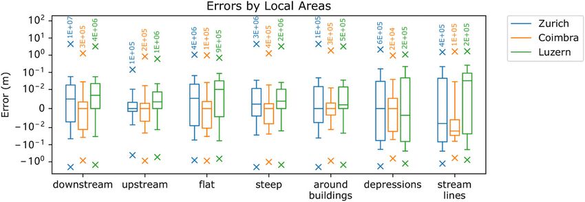
4 of 14                                                                                                         GUO ET AL.

generalize; (b) the patch-based method is an effective        each raster cell and is the directional component of the
way to produce more training data from a limited num-         gradient vector. The curvature is defined as profile curva-
ber of physically-based simulation results; and               ture which describes the acceleration and deceleration of
(c) patches can effectively reduce the input size of the      the flow, and plan curvature which describes the conver-
CNN, easing the CNN training challenges.                      gence and divergence of the flow. Our approach uses the
    The pipeline of the approach can be described as four     difference between these two curvatures (De Smith,
main steps, as presented in Figure 1. First, flood simula-    Goodchild, & Longley, 2007) for simplicity. The mask is a
tions of several design storms in different catchment         binary image that indicates the catchment areas and no-
areas are conducted to produce a flood (maximum water         data areas as 1 and − 1, respectively. The above features
depth) dataset. The obtained water depth results are split    are rescaled linearly to the range of [−1, 1] and
into training and test data sets according to their           concatenated as a multichannel image.
corresponding hyetographs. Second, the elevation data of
the catchment areas are pre-processed into images with
multiple image channels. Each channel corresponds to a        3.3 | CNN-based prediction model
different surface feature. The hyetographs of the design
storms are represented as vectors in which each dimen-        As shown in Figure 2, the prediction network consists of
sion corresponds to the average rainfall intensity in a       a convolutional autoencoder (the main network) and a
5-minute interval. Third, patch locations are randomly        feedforward fully connected neural network (the sub-net-
generated within the catchment area. The patch size           work) that attaches to the main network's latent layer.
equals the input size of the CNN. The patches are used to     The main network and sub-networks process the terrain
train the CNN model by supervised learning, for which         and hyetograph data, respectively. After the latent layer,
the ground truths are the water depth patches, and the        the main network decodes the combined data and pre-
inputs are the corresponding hyetographs and terrain          dicts the water depth values (metres). This type of neural
patches. Finally, after the training, the flood predictions   network that processes data in different formats is usu-
of new storms are performed, but the locations of patches     ally called a joint model (Ngiam et al., 2011).
are sampled from a grid in order to minimize the number           The encoder of the main network is a chain of con-
of necessary patches. The obtained maximum water              volutional modules that consists of three convolutional
depth patches are assembled as the final output.              layers and one pooling layer. The decoder is a chain of
                                                              up-sampling modules that contain one deconvolution
                                                              layer (or formally called transposed convolution layer)
3.2 | Catchment representation                                followed by two convolutional layers. The dimensions of
                                                              the input and output are 256 × 256 × 5 and
Five terrain surface features are included in the terrain     256 × 256 × 1, respectively (height × width × number of
image for catchment representation: elevation, slope,         features). The sub-network consists of one fully con-
aspect, curvature and mask. The slope is defined as the       nected layer and one reshape layer. The size of the fully
magnitude of the gradient vector at each raster cell, rep-    connected layer is 4,096 for convenient concatenation to
resenting the maximum rate of change in value from the        the main network. The kernel sizes are 3 × 3 for all the
centre cell to its neighbours and reflecting the steepness    convolutional layers and 2 × 2 for all the pooling and
of the terrain and the overall movement of the water.         deconvolution layers. We use a small kernel size to pre-
The aspect identifies the direction of the water flow at      serve the thin structure of the terrain and deep layers to

FIGURE 1      Data-driven flood emulation framework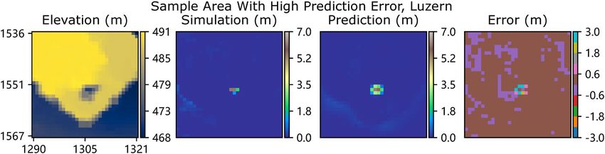
GUO ET AL.                                                                                                          5 of 14

FIGURE 2      The flood prediction network

extend the receptive field (Luo, Li, Urtasun, &               Choosing the grid size is a balance between time and
Zemel, 2016). The activation functions for all the layers     accuracy. Our study investigated four patch aggregation
are Leaky-ReLU (Maas, Hannun, & Ng, 2013) to avoid            options: patches without overlaps, and patches with over-
the “vanishing gradient problem” (Hochreiter, 1998) for       laps aggregated by mean, median, or maximum values,
sigmoid units and the dead neuron problem for rectified       respectively. The grid size for sampling prediction pat-
linear units caused by bad weight initialization (Nair &      ches is 128 (half of the patch size). All results presented
Hinton, 2010).                                                below are obtained using mean values unless mentioned
    Water simulation results usually contain more no-         otherwise.
water and shallow-water areas than deep-water areas,
meaning that the dataset is imbalanced and can lower
the accuracy of deep-water areas. Therefore, a weighted       4 | EXPERIMENTAL SETUP
mean squared error is proposed for the loss function
instead of the standard mean squared error. The defini-       We applied our framework to three different catchment
tion of the loss is given as:                                 areas located in Luzern and Zurich, Switzerland, and
                                                              Coimbra, Portugal, using rasters with a grid size of 1 m.
                     1X y+c                                   The CNN models are trained separately for each catch-
                       e ðy −^yÞ2
                     n                                        ment. The framework was implemented in Python using
                                                              TensorFlow 1.10 (Abadi et al., 2016). All the processes,
where the loss weights are calculated by the exponentia-      including simulation, training, and validation, were per-
tion of the simulated water depth y plus the constant c; ^y   formed with Graphics Processing Unit (GPU) parallel
is the predicted water depth and n is the number of sam-      computing acceleration.
ples. We found that with a larger c, the model tends to
underestimate in deep-water areas. For all the tests in
this paper, we use c = − 1.                                   4.1 | Training data

                                                              To prepare the training data for the experiment, 18 one-
3.4 | Aggregating cell values from                            hour rainfall events were created based on return periods
patches                                                       of 2, 5, 10, 20, 50 and 100 years. Each return period corre-
                                                              sponds to three different events. These events were ran-
The final water depth prediction is aggregated from the       domly labelled as training and test sets except that each
output water depth patches. As already mentioned, the         return period only occurs once in the test set (Figure 3).
patch locations (centre points) are determined by an          The same 18 events were used for the flood simulations
orthogonal grid. The grid size is user-specified and should   in three catchment areas. The CNNs were trained using
not be greater than the patch size. When the grid size        only the training set and were evaluated using the
equals the patch size, the adjacent patches touch each        test set.
other's boundary without overlaps. Smaller grid sizes lead        The simulations were conducted using the CADDIES
to more patches that overlap with each other, which pro-      cellular-automata flood model (Guidolin et al., 2016) for
vides redundant predictions for the overlapping areas to      the Zurich and Luzern catchments, and Infoworks ICM
reduce outliers but increases the computational time.         software (Innovyze, 2019) for the Coimbra catchment.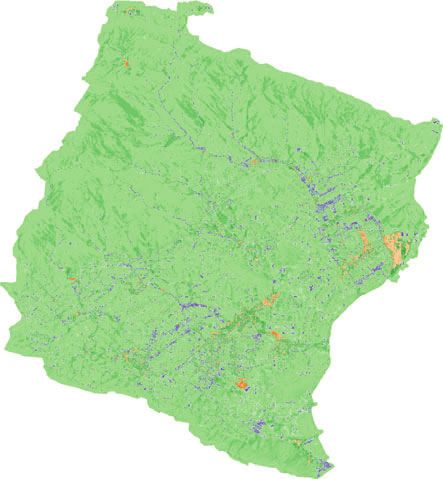
6 of 14                                                                                                              GUO ET AL.

FIGURE 3       Hyetographs used for simulations

CADDIES is a cellular-based surface flood model,                   The accuracy was assessed by the mean absolute error
whereas Infoworks ICM is a physically based model that         (MAE) and the 2D histogram between all the raster cells
can consider coupled pipe/surface flow in urban areas.         of the predicted and simulated water depths. The MAE is
                                                                              P
All the simulations were performed using rasters with a        defined as n1 ni j y^i −yi j , where y^i and yi are the i-th
grid size of 1 m and a minimum time step of 0.01 s.            predicted and simulated raster cells, respectively. We
Bruwier et al. (2018) have suggested that the 90th percen-     used the MAE to assess the accuracy of the results pro-
tile should be used for analysing simulation results in        duced by different meta parameters, such as the patch
order to represent the reality better. However, as we          aggregation methods and the grid size for patch sam-
aimed to replicate the output of a flood simulator, we         pling. The 2D histogram is a plot in which the pixel at
kept the raw simulation outputs without further                row i and column j represents the number of water depth
postprocessing.                                                raster cells that are yi m by prediction and yj m by simula-
    The training data were the hyetograph vectors and          tion. The plot can also be used to show the simulation-
the patches sampled from the terrain elevation data and        error relation by replacing yi to errors. The histograms
the water depth simulations. For each catchment area,          serve as the alternative to scatter plots for better readabil-
10,000 patch locations were randomly sampled. As there         ity. In addition to these two assessment methods, the
are 18 rainfall events created for the dataset, each patch     local performance in different areas such as upstream,
location corresponds to 1 terrain patch and 18 water           downstream and depressions, and the spatial distribution
depth patches. The ground truth data are the water depth       of errors Δy = y^i −yi and relative error δyi = Δyi/yi are also
patches. One flood prediction model was trained for each       reported.
catchment area in order to study the generalizability of           The trained models were also validated using real
CNN on different hyetograph inputs. We used identical          rainfall events1 that were not included in the training
meta parameters to train all models. Specifically, we used     data to further investigate the generalizability of our
the Adam optimizer (Kingma & Ba, 2014) for 200 epochs,         flood prediction model. Real rainfall events that were less
with a batch size of 32 and a fixed learning rate of 0.0001.   than 70 minutes were selected, clipped to 60 minutes,
                                                               and resampled to 12-dimensional vectors. The accuracies
                                                               were reported using histograms as well as spatial plots.
4.2 | Evaluation and validation

The performance of the proposed model was evaluated            5 | RESULTS
based on computational time, prediction accuracy and
the ability of generalization on hyetographs. The compu-       In this section, we present the result of comparing differ-
tational times were measured by repeating the prediction       ent patch aggregation methods as well as the detailed
process and calculating the average time. The time for         analysis of the best patch aggregation method. The latter
necessary pre-processing (e.g., calculating the terrain fea-   consists of the accuracy analysis on the heaviest rainfall
tures) is also reported. In addition, both the accuracy and    event (100-year event) from the test set as well as the vali-
computational time of different aggregation methods            dation on real rainfall events. We chose the heaviest rain
were analysed to discuss the trade-offs between speed          as it could reflect the performance of our model in
and accuracy.                                                  extreme conditions.
GUO ET AL.                                                                                                                                           7 of 14

5.1 | Comparison of the patch                                                   a short conclusion, using the “Mean value” option for
aggregation methods                                                             patch aggregation shows a good balance between accu-
                                                                                racy and prediction time.
5.1.1        |   Computational time

In Table 1, we present the average time of different patch                      5.3 | Prediction accuracy of the best
aggregation methods of our approach. We found that a                            patch aggregation method
trained model significantly reduces the computational
time for water depth prediction compared with that of                           5.3.1 |         Accuracy in shallow and deep
the cellular automata-based models, using only 0.5% sim-                        waters
ulation time. For all three catchment areas, the no patch
overlap option takes the least time. The computation                            The prediction accuracies of the proposed urban pluvial
times of using the mean value and maximum value                                 flood prediction approach in the three catchments are
options are close, and the time difference is less than                         presented as 2D histograms in Figure 5. The first row
6.2% on average. In contrast, the median value option is                        shows the density plots of raster cells with simulated
the slowest because the computer needs to keep all the                          water depth in the x axis and predicted water depths in
data in the memory before the median value can be                               the y axis. The second row are density plots with simu-
obtained.                                                                       lated water depth in the x axis and prediction error in the
                                                                                y axis. The second row plots are essentially the 45 shear
                                                                                of the first row plots, but they are coloured by the ratio of
5.2 | Prediction accuracy                                                       cells in each simulated water depth. The histograms serve
                                                                                as the alternatives of scatter plots for better readability.
The MAEs and the error distributions of the different                           The diagonal and horizontal dots in the plots show the
patch aggregation methods are presented in Figure 4.                            baseline of an ideal model with 100% accuracy - models
The figure shows no significant difference between the                          with higher accuracy are less divergent from the baseline.
results of the different methods and suggests that choos-                       As seen, the histograms clearly show that our model pro-
ing different aggregation methods has negligible effect on                      duces accurate results. The first row of the figure shows a
the accuracy in general. Moreover, the results of rainfall                      higher level of divergence in shallow-water areas than in
events from the test data set do not show higher MAEs                           deep-water areas. But it does not suggest lower accuracy
than those from the training set, suggesting that our                           as the plots are coloured logarithmically and the percent-
model generalizes well with rainfall variations. A more                         age of cells that have an absolute error below 0.1 m is
detailed analysis of the results shows that using over-                         constant (second row in Figure 5).
lapping patches generally results in lower MAEs than
those with the “No overlapping” option. Using the
median value usually gives better results than the Mean                         5.3.2 |         Spatial distribution of errors
and Maximum value options. In addition, the histograms
of the prediction error on the right-hand side of Figure 4                      Figure 6 shows the predicted and simulated water depth
show that the “No overlapping” option generates more                            of the three catchment areas, and Figure 7 shows the
under- and over-predictions in the three catchments,                            corresponding spatial distribution of absolute and relative
suggesting that it generates a large number of outliers. As                     errors (note that the errors are coloured non-linearly so

TABLE 1          Average time performance of the prediction model

                                                             Prediction time (s)a
                                         Pre-
                   Catchment             processing          No                Mean         Median        Maximum          Simulation        Training
    Catchment      size (# pixel)        time (s)            overlapping       value        value         value            time (s)a           timeb (s)
    Luzern         3,369 × 3,110         1.898               0.678 s           2.693 s      14.749 s      2.556 s          2 h 20 min        5 h 25 min
    Zurich         6,175 × 6,050         6.627               1.366 s           5.677 s      75.12 s       5.293 s          4 h 54 min
    Coimbra        1,625 × 2,603         0.636               0.242 s           0.965 s       5.048 s      0.902 s          2 h 18 min
a
 The times are averaged and per rainfall event.
b
 For each catchment area, the amount of training data and training parameters were the same, and identical meta parameters were used; therefore, the average
time is presented.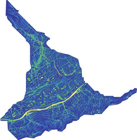
8 of 14 GUO ET AL.
Zurich Zurich
8
Mean Absolute Error no overlaps use mean value 10 no overlaps
use max value use median value use max value
0.035 6
10
Frequency
use mean value
use median value
10 4
0.030
10 2
0.025 10 0
Coimbra Coimbra
no overlaps use mean value no overlaps
Mean Absolute Error
0.025 use max value use median value 10 6 use max value
Frequency
use mean value
use median value
0.020 10 4
10 2
0.015
10 0
Luzern Luzern
10 8
no overlaps use mean value no overlaps
Mean Absolute Error
0.040
use max value use median value use max value
10 6
Frequency
use mean value
0.035
use median value
10 4
0.030
10 2
0.025
10 0
−4 −3 −2 −1 0 1 2 3 4
2-year
5-year
10-year
20-year
50-year
2-year 2
5-year 2
2-year 3
5-year 3
100-year
10-year 2
20-year 2
50-year 2
10-year 3
20-year 3
50-year 3
100-year 2
100-year 3
(test)
(test)
(test)
(test)
(test)
(test)
Error (m)
Rainfall Pattern
F I G U R E 4 The mean absolute errors of each hyetograph (left) and the error histograms of all hyetographs (right) in the Zurich,
Coimbra and Luzern catchments (top to bottom) using different aggregating methods
that the small values can be better visualized). The plots CNN prediction for downstream areas (upper right area
suggest that the CNNs successfully retrieved the spatial shown in Figure 6) than upstream areas (bottom left area
pattern of water depth, showing no significant prediction shown in Figure 6). The accuracy of areas around build-
errors in the different areas. The distribution of errors is ings is also lower than in upstream areas. The hypothesis
relatively even for different areas, with most raster cells is that the CNNs are sensitive for large input values such
an error between −0.1 m and 0.1 m. The relative errors, as the slopes caused by the radical change of elevations
on the other hand, are higher for shallow-water areas next to buildings and other urban features. Another
than deep-water areas. Another observation seen from observation is that the accuracy for places where there is
the enlargement areas is that the CNNs tend to smooth more water than the surroundings, such as streamlines
the output and thus are less accurate for very fine spatial and depressions, is lower compared to other areas of the
scales. catchments. The performance difference between stream-
The model's local performance is presented in lines and depression areas is not significant.
Figure 8, in which catchments are indicated in different
colors. The x marks of the figure are the maximum and
minimum extents of outliers and the numbers on top are 5.3.3 | Analysis of high-error cells
the total number of raster cells of each category. The fig-
ure shows that the performance difference is not signifi- It is noteworthy in Figure 5 that some raster cells that
cant. However, in a more detailed analysis, it can be seen have 0 m water depth in the physically-based simulation
that the model tends to perform better for flat areas results were over-predicted by up to 2 to 3 m. To under-
(slope < 3%) than steep areas (slope ≥ 15%), and for stand what causes such high prediction error, we zoomed
upstream areas (highest 33% terrain elevation) than in to where the errors are larger than 1 m and found that
downstream areas (lowest 33% terrain elevations). For these errors are due to the “smoothing” CNNs make
example, in the Luzern case, raster cells that are dry in around the radical changes of simulated water depths.
simulations are more likely to be marked as wet by the These radical changes seem to be caused by the artefacts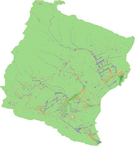
GUO ET AL. 9 of 14
Zurich Coimbra Luzern
7.0 4.0 6.0
10 6 10 6
6.0 10 5 5.0
10 5 3.0 10 5
5.0
Predictions (m)
10 4 4.0
4.0 10 4 10 4
2.0 10 3 3.0
3.0 10 3 10 3
10 2 2.0
2.0 10 2 1.0 10 2
1.0 1.0
10 1 10 1 10 1
0.0 0 0.0 0 0.0 0
0.0 1.0 2.0 3.0 4.0 5.0 6.0 7.0 0.0 1.0 2.0 3.0 4.0 0.0 1.0 2.0 3.0 4.0 5.0 6.0
Simulations (m) 10 0 Simulations (m) 10 0 Simulations (m) 10 0
3.5 2.0 3.0
2.5
10 − 1 10 − 1 2.0 10 − 1
1.0
1.5
1.0
Errors (m)
10 − 2 10 − 2 10 − 2
0.5
0.0 0.0
-0.5 10 − 3 10 − 3 10 − 3
-1.0
-1.5
-1.0
10 − 4 10 − 4 -2.0 10 − 4
-2.5
-3.5 10 − 5 -2.0 10 − 5 -3.0 10 − 5
0.0 1.0 2.0 3.0 4.0 5.0 6.0 7.0 0.0 1.0 2.0 3.0 4.0 0.0 1.0 2.0 3.0 4.0 5.0 6.0
Simulations (m) Simulations (m) Simulations (m)
FIGURE 5 2D histograms that show the density of raster cells. The x axes are simulated water depths and y axes are predicted water
depth (first row) or prediction error (second row). The first row shows the actual number and the second row shows the ratio. Note that the
plots are coloured logarithmically
Zurich Coimbra Luzern
Simulated Water Depth (tr100) Simulated Water Depth (tr100) Simulated Water Depth (tr100)
7.00 m 3.00 m 7.00 m
1.00 m
3.00 m 3.00 m
0.30 m
1.00 m 1.00 m
0.10 m
0.50 m 0.03 m 0.50 m
0.00 m
0.10 m 0.10 m
0.05 m 0.05 m
0.00 m 0.00 m
Predicted Water Depth (tr100) Predicted Water Depth (tr100) Predicted Water Depth (tr100)
7.00 m 3.00 m 7.00 m
1.00 m
3.00 m 3.00 m
0.30 m
1.00 m 1.00 m
0.10 m
0.50 m 0.03 m 0.50 m
0.00 m
0.10 m 0.10 m
0.05 m 0.05 m
0.00 m 0.00 m
FIGURE 6 The simulated (top) and predicted (bottom) water depths of 100-year event for the Zurich, Coimbra and Luzern catchments
(left to right)
10 of 14 GUO ET AL.
Zurich Coimbra Luzern
Spatial Plot of Error (tr100) Spatial Plot of Error (tr100) Spatial Plot of Error (tr100)
0 5.00 m 0 2.00 m 0 5.00 m
0.50 m
1000 500
0.50 m 500 0.50 m
0.05 m
1000
2000
1000 -0.05 m
0.10 m 0.10 m
1500
3000 -0.50 m
1500
-0.10 m -2.00 m 2000 -0.10 m
4000 0 500 1000 1500 2000 2500
2500
5000 -0.50 m -0.50 m
3000
6000
-5.00 m -5.00 m
0 1000 2000 3000 4000 5000 6000 0 1000 2000 3000
Spatial Plot of Relative Error (tr100) Spatial Plot of Relative Error (tr100) Spatial Plot of Relative Error (tr100)
0 500.0 % 0 200.0 % 0 500.0 %
50.0 %
1000 500
50.0 % 500 50.0 %
10.0 %
1000
2000
1000 -10.0 %
10.0 % 10.0 %
1500
3000 -50.0 %
1500
-10.0 % -200.0 %2000 -10.0 %
4000 0 500 1000 1500 2000 2500
2500
5000 -50.0 % -50.0 %
3000
6000
-500.0 % -500.0 %
0 1000 2000 3000 4000 5000 6000 0 1000 2000 3000
FIGURE 7 Errors (top) and relative errors (bottom) of 100-year event for all catchment areas
FIGURE 8 Errors by local areas for all catchment areas
FIGURE 9 The enlargement of the area with the highest prediction error in the Luzern caseGUO ET AL. 11 of 14
in the elevation data. An example of such cases is pres- one model rather than several independent models
ented in Figure 9. Considering that each pixel has a rela- (e.g., Berkhahn et al., 2019). Moreover, validation tests
tively small size (1 × 1 m) compared to the size of the have shown that our model is accurate when provided
catchment area (more than 1,000 × 1,000 m), these errors with “unfamiliar” inputs, suggesting that the
do not affect the interpretation of the prediction result in generalisability of the proposed approach is high. Addi-
practice as: (a) the predicted water depth in the centre is tionally, unlike physically based models, which could
correct; (b) all high-error cells are adjacent to the centre potentially take 10 times more computational time
rather than far from it; (c) a practitioner with experience when doubling the raster resolutions (Guidolin
can quickly identify such errors, and; (d) considering the et al., 2016), the time increase of CNN models is
scale and the short time, predictions containing these expected to be linear as it only correlates with the num-
errors are still of high value. A detailed counting of the ber of input patches.
high-error cells and areas (group of cells with distance Despite the various advantages presented and dis-
between each other less than 16 pixels) is shown in cussed above, several challenges and drawbacks remain
Table 2. These numbers presented in Table 2 can be con- and require further investigations. The main challenge is
sidered small bearing in mind the millions of rasters cells the ability to generalize to different terrain inputs, which
of each catchment. means a CNN model trained on one catchment area can
be used in different catchment areas. Currently, this is
not possible for our model, and to our knowledge, there
5.4 | Validation with real rainfall events are no other models that have achieved this goal.
Another challenge is the lack of large flood datasets due
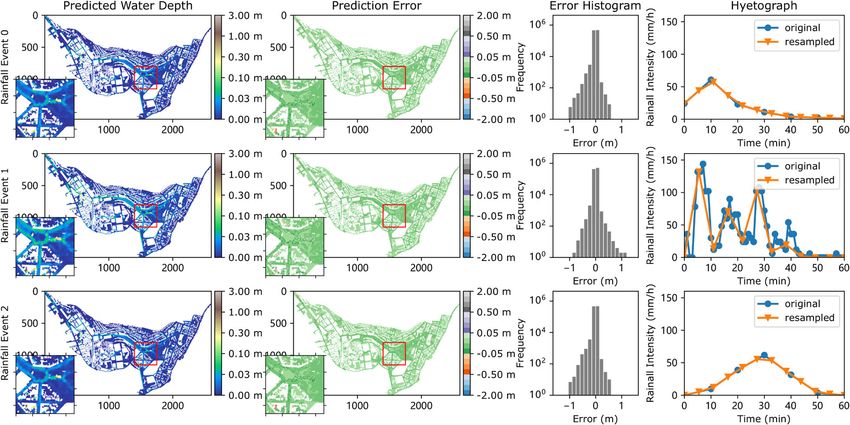
Figure 10 shows the validation results of our model on to the long computational time for simulations and the
three real rainfall events of the Coimbra case. The results difficulty of massively deploying sensors for observational
show that the predictions made by the CNN model are data. This problem can be handled by oversampling and
accurate compared to the simulations. Considering that data augmentation techniques. Data augmentation is also
the real rainfall events contain multiple peaks that did beneficial for the problem of the quality of input data.
not exist in the training data and are thus “unfamiliar” to For example, it is possible to address the problem of low
the CNNs, we can conclude that the model can general- quality or incomplete input data by adding random noise
ize well to different hyetograph inputs and have the to the training data. Another limitation of the proposed
potential to manage arbitrary rainfall patterns. approach is that the input hyetograph vectors have a
fixed length, which is not suitable for rainfall events that
are longer than one-hour. This problem can be solved by
6 | DISCUSSIONS encoding input hyetographs using recurrent neural net-
works (e.g., Chang et al., 2014). Also, recent studies have
In this study we investigated the potential of CNNs to suggested that recurrent neural networks can be
predict urban pluvial flooding using elevation and implemented in a convolution manner to predict flood-
hyetograph data. Compared to other data-driven tech- dynamics directly (Liang & Hu, 2015). Finally, the
niques, the main advantage of CNNs is that they can uti- method presented in this study can still be improved by
lize spatial information and handle inputs of large areas considering other flood relevant factors such as flow
without facing exponential growth of model parameters. velocity. This can be done by adding extra image chan-
Therefore, the entire catchment area can be handled by nels to the output rasters.
TABLE 2 Raster cells with high prediction error for 100-year event in all catchments
Zurich Coimbra Luzern
Absolute Number of Number of Number of Number of Number of Number of
errors (m) cells areas cells areas cells areas
[0.5, 1) 7,949 4,160 210 59 3,140 1,600
[1, 2) 835 354 5 4 212 101
[2, 3) 57 28 0 0 10 4
[3, ∞) 10 4 0 0 2 112 of 14 GUO ET AL.
FIGURE 10 The prediction results of three real rainfall events for the Coimbra case
7 | C ONCLUSIONS A ND F UTURE (Zheng et al., 2018) and computer vision techniques
STEPS (Moy de Vitry et al., 2019).
Computational complexity has been the bottleneck of ACKNOWLEDGMENTS
performing systematic flood analyses using physically This work was funded by the China Scholarship Council
based models. Regarding this challenge, this paper pro- grant 201706090254. The authors would like to thank
poses that maximum water depth predictions can be gen-
Aguas de Coimbra for providing the drainage network
erated using CNNs as an image-to-image translation task information used in this study.
from elevation and hyetograph inputs. The proposed
approach was tested in three different catchment areas, CONFLICT OF INTEREST
and the results showed that the improvement in compu- The authors declare no conflicts of interests.
tational time was substantial and the accuracy was
acceptable for practice purposes. The main contributions DATA AVAILABILITY STATEMENT
of this study are: (a) in contrast to other approaches, the The simulation data, source code and trained models can
proposed model uses spatial information to predict maxi- be obtained from the data repository (Guo, Leit~ao, Sim-
mum urban pluvial flood water depth; (b) the proposed ões, & Moosavi, 2019) hosted by the research collection
model combines both spatial and vector inputs; (c) the of ETH Zurich with DOI link 10.3929/ethz-b-000365484.
obtained results are accurate with the ability to general-
ize to different rainfall inputs, and (d) the proposed ORCID
model can be potentially used to address other relevant Zifeng Guo https://orcid.org/0000-0002-5765-1694
applications without changing the network designs.
For future work, it would be interesting to extend the ENDN OTE
current investigation by combining elevation rasters of 1
The rainfall events were recorded by a rain gauge owned by
different catchments with different hyetographs, produc- Aguas de Coimbra (Portugal) located within the catchment
ing flood prediction models that can generalize to both boundary.
terrain and rainfall inputs. Another interesting direction
would be to train and validate the model using observa- RE FER EN CES
tional data to bypass the issue of long computational time Abadi, M., Barham, P., Chen, J., Chen, Z., Davis, A., Dean, J., … &
for preparing the dataset. This direction is becoming pos- Kudlur, M. (2016). Tensorflow: A system for large-scale
sible through the combination of crowdsourcing methods machine learning. Paper presented at 12th symposium onGUO ET AL. 13 of 14
operating systems design and implementation. USENIX, Savan- Journal of Hydroinformatics, 15(3), 676–686. https://doi.org/10.
nah, pp. 265–283 2166/hydro.2012.245
Bates, P. D., Horritt, M. S., & Fewtrell, T. J. (2010). A simple inertial Chu, M., & Thuerey, N. (2017). Data-driven synthesis of smoke
formulation of the shallow water equations for efficient two- flows with CNN-based feature descriptors. ACM Transactions
dimensional flood inundation modelling. Journal of Hydrology, on Graphics, 36(4), 1–14. https://doi.org/10.1145/3072959.
387(1–2), 33–45. https://doi.org/10.1016/j.jhydrol.2010.03.027 3073643
Berkhahn, S., Fuchs, L., & Neuweiler, I. (2019). An ensemble neu- Greydanus, S., Dzamba, M., & Yosinski, J. (2019). Hamiltonian neu-
ral network model for real-time prediction of urban floods. ral networks. Paper presented at advances in neural informa-
Journal of Hydrology, 575, 743–754. https://doi.org/10.1016/j. tion processing systems 32: Annual conference on neural
jhydrol.2019.05.066 information processing system 2019. Vancouver, Canada,
Bradbrook, K. F., Lane, S. N., Waller, S. G., & Bates, P. D. (2004). pp. 15353–15363.
Two dimensional diffusion wave modelling of flood inundation Guidolin, M., Chen, A. S., Ghimire, B., Keedwell, E. C.,
using a simplified channel representation. International Journal Djordjevic, S., & Savic, D. A. (2016). A weighted cellular autom-
of River Basin Management, 2(3), 211–223. https://doi.org/10. ata 2D inundation model for rapid flood analysis. Environmen-
1080/15715124.2004.9635233 tal Modelling & Software, 84, 378–394. https://doi.org/10.1016/j.
Bruwier, M., Mustafa, A., Aliaga, D. G., Archambeau, P., envsoft.2016.07.008
Erpicum, S., Nishida, G., … Dewals, B. (2018). Influence of Gude, V., Corns, S., & Long, S. (2020). Flood Prediction and Uncer-
urban pattern on inundation flow in floodplains of lowland riv- tainty Estimation Using Deep Learning. Water, 12(3), 884.
ers. Science of the Total Environment., 622-623, 446–458. https://doi.org/10.3390/w12030884
https://doi.org/10.1016/j.scitotenv.2017.11.325 Guo, X., Li, W., & Iorio, F. (2016). Convolutional neural networks
Bui, D. T., Hoang, N. D., Martínez-Alvarez, F., Ngo, P. T. T., for steady flow approximation. Paper presented at the 22nd
Hoa, P. V., Pham, T. D., … Costache, R. (2020). A novel deep ACM SIGKDD international conference on knowledge discov-
learning neural network approach for predicting flash flood ery and data mining. San Francisco, pp. 481–490.
susceptibility: A case study at a high frequency tropical storm Guo Z., Leit~ao J. P., Simões N. E., Moosavi V. (2019). Simulation
area. Science of the Total Environment, 701, 134413. https://doi. data and source code for data-driven flood emulation of urban
org/10.1016/j.scitotenv.2019.134413 flood. ETH Zurich Research Collection. doi: https://doi.org/10.
Chang, F. J., Chen, P. A., Lu, Y. R., Huang, E., & Chang, K. Y. 3929/ethz-b-000365484
(2014). Real-time multi-step-ahead water level forecasting by Hennigh, O. (2017). Lat-net: Compressing lattice Boltzmann flow
recurrent neural networks for urban flood control. Journal of simulations using deep neural networks. arXiv preprint arXiv:
Hydrology, 517, 836–846. https://doi.org/10.1016/j.jhydrol.2014. 1705.09036.
06.013 Hochreiter, S. (1998). The vanishing gradient problem during learn-
Chen, A. S., Djordjevic, S., Leandro, J., & Savic, D. (2007). The ing recurrent neural nets and problem solutions. International
urban inundation model with bidirectional flow interaction Journal of Uncertainty, Fuzziness and Knowledge-Based Systems,
between 2D overland surface and 1D sewer networks. Paper 6(02), 107–116. https://doi.org/10.1142/S0218488598000094
presented at 6th international conference on sustainable tech- Innovyze. (2019). InfoWorks ICM. Retrieved from https://www.
niques and strategies in urban water management innovyze.com/en-us/products/infoworks-icm (accessed July
(NOVATECH 2007), Lyon, France, pp. 465–472. 30, 2019)
De Smith, M. J., Goodchild, M. F., & Longley, P. (2007). Geospatial Jamali, B., Löwe, R., Bach, P. M., Urich, C., Arnbjerg-Nielsen, K., &
analysis: a comprehensive guide to principles, techniques and Deletic, A. (2018). A rapid urban flood inundation and damage
software tools, Leicester, England: . Troubador Publishing Ltd. assessment model. Journal of Hydrology, 564, 1085–1098.
Feng, T., Yu, L. F., Yeung, S. K., Yin, K., & Zhou, K. (2016). Crowd- https://doi.org/10.1016/j.jhydrol.2018.07.064
driven mid-scale layout design. ACM Transactions on Graphics, Jamali, B., Bach, P. M., Cunningham, L., & Deletic, A. (2019). A
35(4), 132. https://doi.org/10.1145/2897824.2925894 Cellular Automata fast flood evaluation (CA-ffé) model. Water
Fewtrell, T. J., Bates, P. D., Horritt, M., & Hunter, N. M. (2008). Resources Research, 55, 4936–4953. https://doi.org/10.1029/
Evaluating the effect of scale in flood inundation modelling in 2018WR023679
urban environments. Hydrological Processes: An International Ladický, L. U., Jeong, S., Solenthaler, B., Pollefeys, M., & Gross, M.
Journal, 22(26), 5107–5118. https://doi.org/10.1002/hyp.7148 (2015). Data-driven fluid simulations using regression forests.
Gao, H., Sun, L., & Wang, J. X. (2020). PhyGeoNet: Physics- ACM Transactions on Graphics, 34(6), 199. https://doi.org/10.
informed geometry-adaptive convolutional neural networks for 1145/2816795.2818129
solving parametric pdes on irregular domain. arXiv preprint Kim, H. I., & Han, K. Y. (2020a). Data-Driven Approach for the
arXiv:2004.13145 Rapid Simulation of Urban Flood Prediction. KSCE Journal of
Gebrehiwot, A., Hashemi-Beni, L., Thompson, G., Civil Engineering, 24(6), 1932–1943. https://doi.org/10.1007/
Kordjamshidi, P., & Langan, T. E. (2019). Deep convolutional s12205-020-1304-7
neural network for flood extent mapping using unmanned Kim, H. I., & Han, K. Y. (2020b). Urban Flood Prediction Using
aerial vehicles data. Sensors, 19(7), 1486. https://doi.org/10. Deep Neural Network with Data Augmentation. Water, 12(3),
3390/s19071486 899. https://doi.org/10.3390/w12030899
Ghimire, B., Chen, A. S., Guidolin, M., Keedwell, E. C., Kingma, D. P., & Ba, J. (2014). Adam: A method for stochastic opti-
Djordjevic, S., & Savic, D. A. (2013). Formulation of a fast 2D mization. Poster presentation in 3rd International Conference
urban pluvial flood model using a cellular automata approach. on Learning Representations (ICLR 2015), San Diego.14 of 14 GUO ET AL.
LeCun, Y., Bengio, Y., & Hinton, G. (2015). Deep learning. Nature, Plate, E. J. (2002). Flood risk and flood management. Journal of
521(7553), 436–444. https://doi.org/10.1038/nature14539 Hydrology, 267(1–2), 2–11. https://doi.org/10.1016/S0022-1694
Leit~ao, J. P., Boonya-Aroonnet, S., Prodanovic, D., & (02)00135-X
Maksimovic, Č. (2009). The influence of digital elevation model Samuels, P. G. (1990). Cross-section location in 1-D models. In
resolution on overland flow networks for modelling urban plu- W. R. White & J. Watts (Eds.), 2nd international conference on
vial flooding. Water Science and Technology, 60(12), 3137–3149. river flood hydraulics (pp. 339–350). Chichester: Wiley.
https://doi.org/10.2166/wst.2009.754 Schuster, M., & Paliwal, K. K. (1997). Bidirectional recurrent neural
Leit~ao, J. P., Zaghloul, M., & Moosavi, V. (2018). Modelling over- networks. IEEE Transactions on Signal Processing, 45(11),
land flow from local inflows in “almost no-time” using self- 2673–2681. https://doi.org/10.1109/78.650093
organizing maps. Paper presented at 11th international confer- Teng, J., Jakeman, A. J., Vaze, J., Croke, B. F., Dutta, D., & Kim, S.
ence on urban drainage modelling (Oral presentation), (2017). Flood inundation modelling: A review of methods,
Palermo, Italy. recent advances and uncertainty analysis. Environmental
L'homme, J., Sayers, P., Gouldby, B., Samuels, P., Wills, M., & Modelling & Software, 90, 201–216. https://doi.org/10.1016/j.
Mulet-Marti, J. (2008). Recent development and application of envsoft.2017.01.006
a rapid flood spreading method. In: Samuels, P., Thuerey, N., Weißenow, K., Prantl, L., & Hu, X. (2020). Deep learn-
Huntington, S., Allsop, W., Harrop, J. (Eds.), Flood risk man- ing methods for Reynolds-averaged Navier–Stokes simulations
agement: Research and practice. Taylor & Francis Group, of airfoil flows. AIAA Journal, 58(1), 25–36. https://doi.org/10.
London, UK. 2514/1.J058291
Liang, M., & Hu, X. (2015). Recurrent convolutional neural net- Tompson, J., Schlachter, K., Sprechmann, P., & Perlin, K. (2017).
work for object recognition. Paper presented at the 28th IEEE Accelerating eulerian fluid simulation with convolutional net-
conference on computer vision and pattern recognition (CVPR works. Paper presented at proceedings of the 34th international
2015), Boston, MA, pp. 3367–3375. conference on machine learning (ICML 2017), Sydney,
Luo, W., Li, Y., Urtasun, R., & Zemel, R. (2016). Understanding the Australia, pp. 3424–3433.
effective receptive field in deep convolutional neural networks. Wang, Y., Fang, Z., Hong, H., & Peng, L. (2020). Flood susceptibility
In Advances in neural information processing systems 29: mapping using convolutional neural network frameworks.
Annual conference on neural information processing systems Journal of Hydrology, 582, 124482. https://doi.org/10.1016/j.
2016, Barcelona, Spain, pp. 4898–4906 jhydrol.2019.124482
Maas, A. L., Hannun, A. Y., & Ng, A. Y. (2013). Rectifier nonlinear- Zaghloul, M. (2017). Machine-learning aided architectural design -
ities improve neural network acoustic models. Paper presented synthesize fast CFD by machine-learning. PhD dissertation.
at the 30th international conference on machine learning ETH Zurich. https://doi.org/10.3929/ethz-b-000207226
(ICML 2013), Atlanta, USA, Volume 30, no. 1, p. 3. Zheng, F., Thibaud, E., Leonard, M., & Westra, S. (2015). Assessing
Moy de Vitry, M., Kramer, S., Wegner, J. D., & Leit~ao, J. P. (2019). the performance of the independence method in modeling spa-
Scalable flood level trend monitoring with surveillance cameras tial extreme rainfall. Water Resources Research, 51(9),
using a deep convolutional neural network. Hydrology and 7744–7758. https://doi.org/10.1002/2015WR016893
Earth System Sciences, 23(11), 4621–4634. https://doi.org/10. Zheng, F., Tao, R., Maier, H. R., See, L., Savic, D., Zhang, T., …
5194/hess-2018-570 Popescu, I. (2018). Crowdsourcing Methods for Data Collection
Mustafa, A., Wei Zhang, X., Aliaga, D. G., Bruwier, M., Nishida, G., in Geophysics: State of the Art, Issues, and Future Directions.
Dewals, B., … Teller, J. (2018). Procedural generation of flood- Reviews of Geophysics, 56(4), 698–740. https://doi.org/10.1029/
sensitive urban layouts. Environment and Planning B: Urban 2018RG000616
Analytics and City Science, 47, 889–911. https://doi.org/10.
1177/2399808318812458
Nair, V., & Hinton, G. E. (2010). Rectified linear units improve How to cite this article: Guo Z, Leit~ao JP,
restricted Boltzmann machines. Paper presented at the 27th Simões NE, Moosavi V. Data-driven flood
international conference on machine learning (ICML 2010),
emulation: Speeding up urban flood predictions by
Haifa, Israel, pp. 807–814
Ngiam, J., Khosla, A., Kim, M., Nam, J., Lee, H., & Ng, A. Y. (2011).
deep convolutional neural networks. J Flood Risk
Multimodal deep learning. Paper presented at the 28th interna- Management. 2021;14:e12684. https://doi.org/10.
tional conference on machine learning (ICML 2011), Bellevue, 1111/jfr3.12684
pp. 689–696You can also read