Computers and Geosciences
←
→
Page content transcription
If your browser does not render page correctly, please read the page content below
Computers & Geosciences 158 (2022) 104962
Contents lists available at ScienceDirect
Computers and Geosciences
journal homepage: www.elsevier.com/locate/cageo
Updating geostatistically simulated models of mineral deposits in real-time
with incoming new information using actor-critic reinforcement learning
Ashish Kumar *, Roussos Dimitrakopoulos
COSMO – Stochastic Mine Planning Laboratory, Department of Mining and Materials Engineering, McGill University, FDA Building, 3450 University Street, Montreal,
Quebec, H3A 0E8, Canada
A R T I C L E I N F O A B S T R A C T
Keywords: The existing technologies that update geostatistically simulated models of mineral deposits cannot self-learn from
Data assimilation incoming new information generated in operating mines and do not account for high-order spatial statistics. This
High-order spatial statistics work proposes a novel self-learning artificial intelligence algorithm that learns from incoming new information
Geostatistics
and accounts for high-order spatial statistics, in order to update the geostatistically simulated models of mineral
Reinforcement learning
Real-time
deposits in real-time. The proposed algorithm uses deep policy gradient reinforcement learning with an actor and
Production sensor data a critic agent. The grid nodes of the geostatistically simulated model are visited sequentially in a random path,
Convolutional neural network the environment generates the states for each grid node, and feeds the state to the actor and critic agents that
respectively predict and evaluate the updated property of the grid node The data is stored in a replay memory,
which is sampled at regular intervals to train the agents. The trained agents are then used for further rounds of
self-learning. An application of the proposed algorithm at a copper mining operation with incoming drilling
machine sensor data (collected spatially), and processing mill sensor data (collected over time), demonstrates its
applied aspects in updating the geostatistically simulated models of copper grades of the mineral deposit in real-
time, while also reproducing spatial patterns and high-order spatial statistics.
1. Introduction new information, referred to as “soft data”, is partial and noisy, and is
therefore uncertain. The soft nature of the new information is attributed
New information is readily available with conventional and new to the characteristics of the related sensors that generate indirect mea
digital technologies that are used during production activities in in surements compared to, for example, those derived from the analysis of
dustrial environments. These technologies include advanced sensors and drillhole samples in geochemical laboratories. Assimilating incoming
monitoring devices that are used during production activities in mines new information in simulations is similar to history matching in petro
and oilfields, and in monitoring activities in the fields of hydrogeology, leum reservoirs (Gilman and Ozgen, 2013; Oliver et al., 2008). History
hydrology, meteorology, atmospheric sciences, geomorphology and matching entails using production data such as oil production, flow rates
oceanography. For example, in an industrial mining environment, global and well pressure to update simulations of static reservoir properties,
positioning systems can locate and monitor the status of the mining fleet such as porosity and permeability, along with dynamic reservoir prop
in real-time (Chaowasakoo et al., 2014). Built-in control units can erties, such as pressure and fluid saturation, to better match the
monitor the health and utilization of the mining fleet (Koellner et al., observed production data.
2004). Radiofrequency identification tags can locate and track the flow Ensemble Kalman filter (EnKF) is a thoroughly studied and applied
of materials from mines to customer (Rosa et al., 2007), and infrared and method for history matching in petroleum and groundwater reservoirs
X-ray sensors can measure the geological properties of the materials that (Aanonsen et al., 2009; Conjard and Grana, 2021; Oliver and Chen,
are mined, hauled, conveyed, processed and sold (Dalm et al., 2018; De 2011; Xu et al., 2013). Benndorf (2020, 2015) introduced the use of the
Jong, 2004; Goetz et al., 2009; Iyakwari et al., 2016). The incoming new EnKF for updating geostatistically estimated models of mineral deposits.
information is typically used to update the relevant properties of geo Yüksel et al. (2017, 2016) used the EnKF method to update simulations
statistically simulated models (hereafter, simulations). However, this of ash content with incoming new information at a coal deposit.
* Corresponding author. Vale, Digital Transformation Department, 2060 Flavelle Boulevard, Mississauga, Ontario, L5K 1Z9, Canada.
E-mail addresses: ashish.kumar@mail.mcgill.ca (A. Kumar), roussos.dimitrakopoulos@mcgill.ca (R. Dimitrakopoulos).
URL: https://github.com/ashishrokz1993/MineralDepositAICG (A. Kumar).
https://doi.org/10.1016/j.cageo.2021.104962
Received 14 June 2020; Received in revised form 16 September 2021; Accepted 6 October 2021
0098-3004/© 2021 Published by Elsevier Ltd.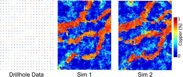
A. Kumar and R. Dimitrakopoulos Computers and Geosciences 158 (2022) 104962
Wambeke and Benndorf (2017) proposed a combination of the EnKF sections, first the proposed self-learning AI algorithm is detailed. Next,
method with a forward simulator, while incorporating a connected an application at a synthetic copper mining operation is explored to
updating cycle and a local neighborhood technique, to update the sim illustrate the efficiency and applied aspects of the proposed algorithm.
ulations with the sensor data collected from the conveyor belt at a Conclusions and directions for future research follow.
synthetic mining operation. Wambeke and Benndorf (2018) studied the
effect of measurement volumes, blending ratios and sensor precision 2. Method
within the EnKF method. Wambeke et al. (2018) used a forward simu
lator and Bond’s work theorem with the EnKF method to update the Section 2.1 provides the notations used throughout this section.
simulations of the Bond work index – a geometallurgical property – at Section 2.2 details how new information is collected during day-to-day
the Tropicana gold mine with the processing mill sensor data about production activities in a mining operation that transform raw materials
throughput, power draw, feed and product size. Other methods for to products. Section 2.2 provides the details of the proposed self-
updating simulations of pertinent properties in a mineral deposit include learning AI algorithm. Section 2.3 details the process of using the pro
co-simulation with soft data (Journel and Alabert, 1990; Neves et al., posed algorithm in an operating mining environment.
2018) and conditional simulation by successive residuals (Jewbali and
Dimitrakopoulos, 2011; Vargas-Guzmán and Dimitrakopoulos, 2002). 2.1. Notations
Methods such as gradual deformation (Hu, 2000), neighborhood algo
rithm (Sambridge, 1999), evolutionary algorithm (Schulze-Riegert and Table 1 shows the sets, indices, and constants and Table 2 presents
Ghedan, 2007), maximum a posteriori (Oliver, 1996), Markov chain the variables used in the proposed algorithm.
Monte Carlo (Fu et al., 2017; Oliver et al., 1997), inverse sequential
simulation (Xu and Gómez-Hernández, 2015), classification and 2.2. Incoming new information in a mining operation and related
regression tree algorithm (Gutiérrez-Esparza and Gómez-Hernández, notations
2017), randomized maximum likelihood (Chen and Oliver, 2012; Sarma
et al., 2006; Vo and Durlofsky, 2014), Tau-model (Naraghi and Srini Let Z(u) be a spatial random field with random variables Z(x), rep
vasan, 2015), Markov mesh model (Panzeri et al., 2016), variants of the resenting a property of a mining block at location x, with x = 1, …, N
ensemble Kalman filter and co-simulation with soft data (Ángel et al., being the index of the blocks. For example, without loss of generality
2021; Journel and Alabert, 1990; Li et al., 2021; Mao and Journel, and for simplicity let’s assume that the grid shown in Fig. 1(a) represent
1999a; Soares et al., 2017) have also been used for updating simulations Z(u). Initial direct measurements, І, derived from the analysis of
of pertinent properties of petroleum and groundwater reservoirs. The exploration drillhole samples in geochemical laboratories is denoted by
above-mentioned methods update the relevant properties of simulations DI as shown in Fig. 1(a). A finite set of initial simulations, SI , is gener
but do not learn from the incoming new information. Learning from new ated using DI , that represent realizations, zs (u) of Z(u), and quantify the
information refers to extracting complex patterns and relationships be uncertainty about the spatial property of materials in the mine as shown
tween new information and simulations, while maintaining this infor in Fig. 1(b).
mation for future use. Additionally, they do not account for nor respect The sensors installed on the drilling machines, B, located spatially
high-order spatial statistics while updating the simulations. within the mine, measure the quality of materials drilled. The new in
Recent developments in history matching include artificial intelli formation, NІ, generated spatially by the sensors on the drilling machine
gence (AI) algorithms based on supervised machine learning, such as a about the property of a block, Z(x), within the mine is denoted by NIB (x).
convolutional neural network (CNN) with principal component analysis The blasted materials are then loaded with shovels, S, into trucks, T. The
(PCA) (Liu et al., 2019) and stepwise CNN-PCA with recurrent neural sensors on the shovels measure the quantity, qi (x), and quality, NIi (x),
network (RNN) (Tang et al., 2019). The CNN-PCA method trains a CNN ∀i ∈ S, of a block, Z(x), loaded. The sensors on the truck measure the
to post-process a given PCA geostatistical model, which involves using a
quantity, qi (x), and quality, NIi (x), ∀i ∈ T, of Z(x) hauled. The incoming
training dataset to learn to minimize the difference between the style
new information about the quality of blocks Z(x) located spatially within
and content of the generated post-processed PCA model, and the target
the mine is herein referred to as “spatial sensor data” and denoted by
style and content calculated from either a training image or an initial
S ∈ B ∪ S ∪ T as shown in Fig. 1(c). The trucks haul the materials to
simulation. The CNN-PCA-RNN trains an RNN to generate flow simu
different destinations, D as shown in Fig. 1(d). Let f d , ∀d ∈ D represent a
lation results for given simulations of porosity and permeability, and
function that mimics the transformation of materials at destination d.
involves using a training dataset to learn to minimize the difference
between the predictions of the RNN and the targets generated by a The sensors at the destinations measure the quality NId (qd ), ∀d ∈ D, and
high-fidelity flow simulator. These methods aim to minimize the quantity, qd , of materials at destination d. For example, a destination in a
mismatch between the targets and generated outputs for a given training mining operation can be crusher as shown in Fig. 1(e) which has sensors
dataset and, therefore, cannot perform well if the inputs differ greatly to monitor the quality and quantity of materials. The materials from the
from the training dataset. destinations are transported via conveyor belts, C, to processing streams,
The work presented herein, which is inspired by the continuous P. The conveyor belt analyzer monitors the rate, qd,p,c , and quality,
control algorithm (Lillicrap et al., 2015), proposes a novel self-learning NIc (qd,p,c ), ∀d ∈ D, p ∈ P, c ∈ C, of material transported via conveyor c
AI algorithm that trains agents (typically function approximators like from destination d to processing stream p. For example, the materials
neural networks) to update simulations of pertinent properties of min from crusher is transported to processing mill via a conveyor belt and
eral deposits in real-time with new incoming information. The proposed analyzed via a conveyor belt analyzer as shown in Fig. 1(f). The pro
algorithm uses deep deterministic policy gradient reinforcement cessing streams generate the products which are sold to customers as
learning with an actor and a critic agent (in this work, both are CNN) to shown in Fig. 1(g). Let f p , ∀p ∈ P denote the function that mimics the
learn about the relationships between incoming new information and transformation of materials at processing stream p. The sensors at the
simulations. These relationships are defined by high-order spatial sta processing stream measure the quality, NIp (qp ), and quantity, qp , ∀p ∈ P,
tistics. High-order spatial statistics (Dimitrakopoulos et al., 2010; Min of products generated as shown in Fig. 1(g). Let T represent a set that
niakhmetov et al., 2018; Minniakhmetov and Dimitrakopoulos, 2021; consists of all the components in a mining operation that handle and
Mustapha and Dimitrakopoulos, 2011; Yao et al., 2021a, 2021b) can process the materials and collect sensor data, i.e. T = {D, C, P}. Let
capture complex spatial geological characteristics, curvilinear features, NIi (qi ) and qi represent the incoming new information collected over
geometric relations and the connectivity of extreme values needed for time with sensors at component i ∈ T about the quality and quantity of
updating spatially dependent geological phenomena. In the following related materials, referred to herein as “temporal sensor data”. For
2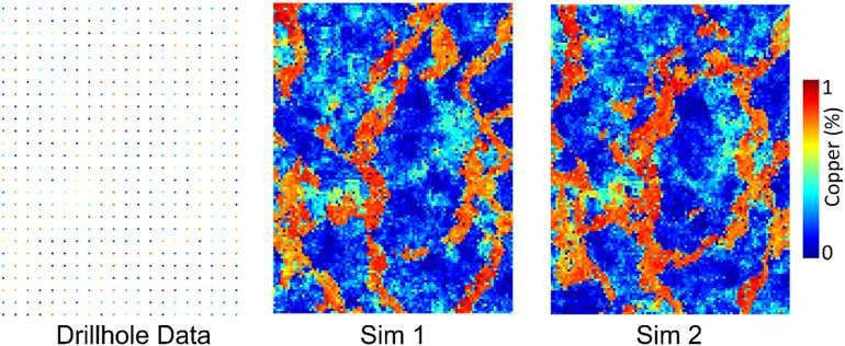
A. Kumar and R. Dimitrakopoulos Computers and Geosciences 158 (2022) 104962
Table 1 Table 1 (continued )
Sets, indices, and constants used in the proposed algorithm. Parameters Definition
Parameters Definition
NBS
Z(u) Spatial random field consisting of random variables Z(x), ∀x ∈ [1, γ Discount factor
N] NR Replay memory cache size
Z(x) Random variable representing a property of a mining block at NI Training interval
location x, ∀x ∈ [1, N] within the mine
γMP
i
The adjxustment factor for adjusting the magnitude of model-based
DI Initial (I) drillhole (D) samples at the mine prediction error
SI Set of initial simulations generated usingDI for all blocks in Z(x) c L2 regularization cost
Zs (x) Simulated property of a block located at x in s ∈ SI NU Update training iterations
SU Set of updated simulations for all blocks within the mine; s ∈ SU
′ NTE Number of training episodes
U NT Number of training iterations
Zs (x) Simulated property of a block located at x in s ∈ S
′ ′
NUE Number of update training episodes
B, T, S, D, C, P Set of blasthole drilling machines (B), trucks (T), shovels (S),
destinations (D), conveyor belts (C), and processing streams (P),
respectively in a mining operation
NIB (x) New information (NI) generated spatially by sensors located on B
Table 2
about the quality of material drilled
Variables used in the proposed algorithm.
q (x), NIi (x)
i New information generated spatially about the quantity and
quality of materials, respectively at component i ∈ S ∪ T Variable Definition
S Set of sensors that generate spatial new information, i.e. S ∈ B ∪ fθ μ Actor agent (a CNN) parameterized by θμ
S∪T fθQ Critic agent (a CNN) parametrized by θQ
qd , NId (qd ) Temporal new information generated by the sensor at destination
st State at time t
d ∈ D about the quantity and quality of materials, respectively
at Action proposed by actor agent at time t
fd A function that mimics the transformation of materials at
destination d ∈ D rt Reward computed by the environment at time t
d,p,c Temporal new information generated by the sensor at conveyor t Random noise process added to the actions at time t, for exploration
q
N
,
belt c ∈ C about the quantity and quality of materials, respectively during training
NIc (qd,p,c )
transported from destination d ∈ D to processing stream p ∈ P fθQ Target critic CNN agent parameterized by θQ
′ ′
p p
q , NIp (q ) Temporal new information generated by the sensor at processing fθμ Target actor CNN agent parameterized by θμ
′ ′
stream p ∈ P about the quantity and quality of materials,
respectively
fp A function that mimics the transformation of materials at
processing stream p ∈ P
example, in Fig. 1 the temporal sensor data will be generated from a
crusher, a conveyor belt and a processing mill. The tracking devices
T Set of sensors that generate temporal new information, i.e. T ∈
D∪C∪P installed on component i ∈ T ∪ S of the mining operation, help to
Track Sensors that tracks the flow of materials from mine to customer locate and track the flow of materials. Let Track represent an operator
Neighx The neighborhood of a mining block located at x that can locate and track the flow of materials from the mine to the
Zs (Neighx ) Simulated property of all the block in s inside Neighx customers. For example, the materials flowing from mine to customer in
Simulated property of all the block in s inside Neighx
Fig. 1(d–g) is tracked using the RFID tags in the blastholes and GPS
Zs (Neighx )
′ ′
installed on trucks. Track operator for this example will represent the
Dsx Conditioning data event value for a block located at x in s
′ ′
data generated by RFID sensors and GPS about the location of materials
Ns Number of conditioning values in the data event in s ∈ SI while it flows from mine to customer.
Nsζ Number of replicates for data event Dsx found in s within Zs (Neighx )
′
Value of node j ∈ Ns in the replicate i ∈ Nsζ 2.3. A self-learning AI algorithm
′
ζs,i,j
Hsx The geometry of conditioning data event Dsx defined by a
′ ′
normalized three-dimensional distance vector found in s ∈ SI The proposed self-learning AI algorithm for updating the simulations
NIS (Neighx ) Spatial sensor data collected inside Neighx of pertinent properties of mineral deposits with incoming new infor
DSx Conditioning data event value for block located at x in S mation uses deep deterministic policy gradient (DDPG) reinforcement
NS Number of conditioning values in the data event in S learning (Lillicrap et al., 2015) with an actor and a critic agent (in this
NSζ Number of replicates for data event DSx found in S within work, both are CNN). The actor, μ, and critic, Q, agents (fθμ , and fθQ
NIS (Neighx ) parametrized by θμ , and θQ , respectively) interact with an environment
ζS ,i,j Value of node j ∈ NS in the replicate i ∈ NSζ (see Sect. 2.3.1 for details of the environment) in discrete timesteps.
HSx The geometry of conditioning data event DSx defined by a Herein, a time step t denotes the point at which a block is visited along a
normalized three-dimensional distance vector found in the S random path visiting all blocks, similar to the sequential simulation
V(zs (x)) The conditional variance of a block located at x computed over SI approach (Deutsch and Journel, 1992; Gómez-Hernández and Srivas
Esx Average conditional variance for a block located at x over s ∈ SI tava, 2021; Journel, 1994). At each time step t the actor takes an action
inside Neighx at ∈ R which is to predict the updated property Zs (x) of a block located
′
γs Adjustment factor to adjust the magnitude of Esx at x based on a state, st – which is fully observable – for a given simu
E(NIS (x)) The error of spatial sensor data for a block located at x lation s ∈ SI . The action is executed in an environment, meaning that
ENI
x
S Average error with the spatial sensor data in the neighborhood the block property, Zs (x), is updated with the taken action at to generate
Neighx of a block located at x
an updated simulation s ∈ SU and the agent receives a scalar reward rt
′
ENIi Error in the new information collected from the component i ∈ D ∪
C ∪ P in a mining operation and a next state st+1 (see Sect. 2.3.1 for calculation of rt and st+1 ). The
W Legendre series polynomial order for the approximation of process continues until all the blocks are visited and updated. The state,
conditional probability distribution function action, reward, next state tuple (st at , rt , and st+1 respectively) from all
τ The soft target update parameter the time steps is stored in a replay memory buffer, R, of finite-sized
Batch size cache. The replay memory is sampled uniformly at regular intervals to
train both the actor and critic agents (see Sect. 2.3.3 for the training of
3
A. Kumar and R. Dimitrakopoulos Computers and Geosciences 158 (2022) 104962
Fig. 1. (a) Exploration drillhole data; (b) set
of initial simulations generated using the
exploration drillhole data; (c) spatial sensor
data collected via sensors installed on dril
ling machines, shovels and trucks; (d) GPS
and RFID tags help to track which blocks are
extracted from the mine and sent to crusher;
(e) sensor at the crusher measure quality and
quantity of crushed materials; (f) sensors on
conveyor belt measure rate and quality of
conveyed materials, and (g) sensor at the
processing mill measure the quality and quantity of processed materials.
actor and critic agents). The algorithm terminates when NT iterations simple example as shown in Fig. 2. Suppose Zs (Neighx ) and x are
are reached, and the trained actor agent fθμ can be used to update the respectively represented by the dashed box and black circle in Fig. 2(a),
simulations SU , of pertinent properties of mineral deposits with the new then the ends of black arrows in Fig. 2(b) constitutes Dsx .
′
information collected during production activities in a mining operation The third component of the state is the incoming spatial new infor
as detailed in Sect. 2.4. mation S including and surrounding a block located at x, denoted by
NIS (Neighx ). The absent values in the spatial new data are initialized to
2.3.1. Environment − 1. The fourth component of the state is the conditioning data event DSx
In the context of the present study, an environment is a model of the found in the spatial sensor data which includes the NS closest spatial
mining operation that encapsulates how materials are extracted from sensors’ data. Suppose NIS (Neighx ) and x are respectively represented
the mines are transformed from raw materials to products with pro by the dashed box and the black circle in Fig. 2(c), then the ends of black
duction activities. The agents interact with the environment by visiting
arrows in Fig. 2(c) constitutes DSx . The quantity of conditioning data NS
mining blocks in a random path. The environment provides a repre
is computed based on the density of the spatial sensor data. The fifth
sentation of the mining operation during its interaction with the agents.
component of the state is the geometry of the conditioning data events
The representation is called a state, and includes information such as the
Dsx and DSx ,defined by normalized distance vectors Hsx and HSx ,
′ ′
property of blocks in initial simulations, conditioning data events and
geometry, new information, conditional variance of the blocks in the respectively (the distance of the conditioning data point from a block
initial simulations, error in the new information, and the model-based located at x). The sixth component of the state is the average conditional
predictions. The environment is also responsible for evaluating and variance Esx associated with a property of a block located at x in s ∈ SI
using the action at taken by the agent to generate a scalar value rt , called inside Neighx . Esx is calculated as:
a reward, and a new representation, called the next state st+1 . The γs ∑
calculation of the state, reward, and next state in the environment are Exs = V(Z s (xi )), ∀s ∈ SI (1)
|Neighx | i∈Neighx
detailed next.
where, V(Zs (xi )) is the conditional variance of the initial simulated
2.3.1.1. State. The state st generated by the environment is comprised property of a block xi and γ s is an adjustment factor to adjust the
of 10 components. The first component is the property of the blocks in magnitude of the conditional variance of the simulations. The seventh
the initial simulation s ∈ SI including and surrounding the block located component of the state is the error in the spatial sensor data ENI x
S
at x in consideration at time step t denoted by Zs (Neighx ). Here, Neighx collected in Neighx of a block located at x. The error with each of the
defines the neighborhood to consider around a block located at x, and is spatial sensor data is an input to the algorithm. ENI S is computed by
x
an input for the algorithm. The missing blocks in Neighx are initialized to averaging the error in the available spatial sensor data in Neighx as:
− 1. For example, the neighborhood for the blocks close to the edges of
∑
the simulation grid will go outside the grid and, thus, these blocks are ExNIS =
1
E(NIS (xi )) (2)
called missing blocks and are initialized to − 1. The second component of |Neighx | i∈Neighx
the state is the conditioning data event Dsx which includes a property of
′
The eighth component of the state is the incoming temporal sensor
Ns closest blocks for a block x in s ∈ SU . s is formed by first creating a
′ ′
data, qi ,NIi (qi ), ∀i ∈ T . The ninth component of the state is the errors in
I
copy of s ∈ S and then updating the simulated property of blocks that the temporal sensor data, ENIi , ∀i ∈ T , and is an input to the algorithm.
have been visited until time t − 1 with the actions taken by the actor Let’s consider a simple example as shown in Fig. 3 where mining blocks
agent. This captures the history of actions taken until t − 1. The quantity 11 and 39 are entirely extracted on day 1 and blocks 20 and 34 are
of conditioning data Ns is an input for the algorithm. Let’s consider a entirely extracted on day 2 The extracted materials are transported to
Fig. 2. State representation of (a) a property of the blocks in the neighborhood Neighx of a block located at x in consideration at time step t in the initial simulation
s ∈ SI ; (b) conditioning data event found in the simulation s ∈ SU until t − 1; and (c) spatial sensor data with its conditioning data event.
′
4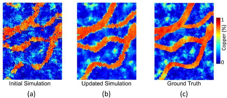
A. Kumar and R. Dimitrakopoulos Computers and Geosciences 158 (2022) 104962
Fig. 3. State representation of incoming temporal sensor data and its associated errors in measurements.
crusher 1 and thereafter to the mill 1. The GPS on the truck and the RFID 2.3.1.3. Action. The state st is fed to the actor agent, fθμ , to generate an
tags in the blastholes of those blocks will help to track the material by action at ∈ R+ as shown below:
generating origin and destination data as shown in Fig. 3. To ensure that
at = fθμ (st ) + N (6)
tracking of materials from mining blocks to destinations data is appro t
priate and useful, a mining operation needs to ensure that issues related
where, N t is the noise added to the action to ensure exploration during
to dilution and selective mining units are properly addressed as dis
the training phase of the proposed AI algorithm. The action at is to
cussed in Parker (2012). The sensor installed on the conveyor belt CB1
predict the updated property, Zs (x), of a block located at x based on a
′
measure the grade of materials passing on the conveyor belt along with
an associated error for such measurements. The tenth component of the state st in a simulation s ∈ SI .
state is the model-based prediction for the updated simulation s ∈ SU at
′
the location of the different temporal sensor data (see Sect. 2.3.1.2 2.3.1.4. Next state. The next state st+1 is generated by first replacing
shows details of how model-based prediction is generated). Calculating Zs (x) in Zs (Neighx ) with the action at taken by the actor agent to form
the model-based prediction for the updated simulation captures the Zs (Neighx ), and then generating the model-based prediction with Zs (x).
′ ′
history of the actions taken until time step t − 1. If there are no new The rest of the information in the next state st+1 remains the same as in
temporal sensor data, then such data along with their model-based the state st .
predictions are initialized to − 1.
2.3.1.5. Reward. The action at taken by the agent in the state st is
2.3.1.2. Model-based predictions. Model-based predictions, MP, calcu evaluated by the environment to generate a reward rt . The reward rt
late the values that should have been observed based on simulations at leverages high-order spatial statistics and consists of three parts, as
the location where temporal sensor data was collected. The model-based shown below:
prediction MPsd at a destination d for a simulation s is calculated with Eq ∑
(3). rt = rs,t + rS ,t + ri,t (7)
i∈T
( )
s
MPd = f d
∑
Track(qi (x); Z (x)) , ∀s ∈ SI , d ∈ D
s
(3) The first part, rs,t , evaluates the likelihood of at in the conditional
i∈T probability distribution function (CPDF), which is generated by
searching for replicates of a conditioning data event Dsx within a simu
′
Equation (3) uses the Track operator first to find the quantities of
materials, qi (x), ∀i ∈ T, hauled with trucks i ∈ T to a destination d then lation. The second part, rS ,t , evaluates the likelihood of an action at in
utilizes the function f d to calculate how the materials are transformed at the CPDF, which is generated by searching for replicates of DSx within
the destination, and finally uses the simulated property Zs (x) along with the spatial sensor data. The third part, ri,t , ∀i ∈ T , computes the error
the tracking and transformation data to compute MPsd . The model-based between a model-based prediction and temporal sensor data for at . The
prediction MPsc for a simulation s at a conveyor belt c which transports CPDF of a given conditioning data event is generated using high-order
materials from a destination d to a processing stream p is calculated as: spatial Legendre moments (Dimitrakopoulos et al., 2010; Mustapha
( ) and Dimitrakopoulos, 2011; Yao et al., 2018). High-order spatial Leg
MPsc = Track MPsd sqd,p,c , ∀s ∈ SI , d ∈ D, p ∈ P, c ∈ C (4) endre moments capture multi-point spatial statistics and approximates
the CPDF of the center node Z(x) for a data event Dsx using Legendre
′
Equation (4) first uses the Track operator to find the quantity of
material qd,p,c flowing from a destination d to a processing stream p with polynomials. The initial simulated property Zs (Neighx ) inside Neighx is
searched for all available replicatesNζs , of Dsx , defined by a distance
′
conveyor belt c and then utilizes the model-based prediction from Eq.
(3) along with the tracking information to compute MPsc . For example, in vector, Hsx . Let ζs,i,j denote the values of each node j ∈ Ns in the replicate
′
Fig. 3, Track represent the origin and destination data, qi (x) for blocks 11 i ∈ Nsζ . The replicates ζs,i,j are used to compute the CPDF of the center
and 39 extracted on day 1 is 1 (since the block is extracted entirely),
node Z(x) with Legendre polynomials as:
Zs (x) is the value of blocks 11 and 39 in simulation s, f d is a summation ∑ ∏ ( )
function for simplicity, and qd,p,c is 2 blocks per day. The model-based ( ⃒ ′) ( ) i∈Nζs Xi (Z(x))s j∈N s Xi ζ s,i,j
, ∀s ∈ SI (8)
′
fs Z(x)⃒Dsx ≈ f̃ W Z(x)|Ds = ∑ ∏ ( )
prediction MPsp at a processing stream p for a simulation s is calcu s x
i∈N s j∈N s Xi ζ s,i,j
lated as follows:
ζ
(
∑
) where,
( )
MPsp = f p Track MPsc , ∀s ∈ SI , p ∈ P (5) W ( )
∑ 1 ( )
c∈C
Xi (Z(j)) = w+ Pw ζs,i,j Pw (Z(j)) (9)
2
Equation (5) first uses the Track operator to find the quantity of w=0
materials fed to a processing stream with different conveyors, then uses W is the degree of the Legendre polynomials. Pw (Z(x)) is the wth-
the function f p to find how materials are transformed into products, and degree Legendre polynomial for center node Z(x) calculated as follows:
finally uses the model-based prediction from Eq. (4) along with the
tracking and transformation information to compute MPsp .
5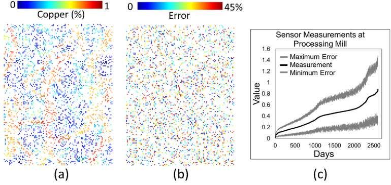
A. Kumar and R. Dimitrakopoulos Computers and Geosciences 158 (2022) 104962
1 dw [( )w ] calculated using Eqs. (3)–(5). The additional data are not added as in
Pw (Z(x)) = Z(x)2 − 1 (10)
2w w! dZ(x)w puts until the fully connected layer in the actor agent, as shown in Fig. 4
(a). The actor agent takes an action at based on the state st , which is to
For more details on the computation of CPDF with high-order spatial
predict the updated simulated property Zs (x) of a block located at x. The
′
Legendre moments, readers are referred to Mustapha and Dimi
trakopoulos (2011) and Yao et al. (2018). The first part of the reward critic agent, fθQ , is also a CNN, which takes as input the state st and as an
calculation is therefore calculated as: additional input the action taken by the actor agent. Similar to the actor
( ( )) agent, the additional data and the action are not added as inputs until
⃒ ′) (
(11) the fully connected layer in the critic agent as shown in Fig. 4(b). The
′ ′
W Z(x) = Z s (x)⃒Ds − f̃
rs,t = λs ⋅ f̃
s x
W s s
s Z(x) = Z (x)|Dx , ∀s ∈ SI
critic agent is an action-value function which evaluates the action at
where, taken by the actor agent in the state st .
1 − Exs 2.3.3. Actor-critic training
λs = ∑ , ∀s ∈ SI (12)
1 − Exs + 1 − ExNIS + i∈T 1 − ENIi The actor and critic agents are trained using DDPG reinforcement
λs is the weight associated with reproducing the spatial statistics of learning, as shown in Fig. 5. The agents are initialized randomly at time,
the initial simulation s. The second part of the reward calculation, rS ,t , t = 1, with weights, θμ and θQ , respectively. In addition to the actor and
which defines the likelihood of action at compared to the initial simu critic agents, two target agents (target actor and target critic), denoted
⃒
by fθμ , and fθQ , and parametrized by θμ and θQ , are created to avoid
′
lated property Zs (x) in the CPDF fS (Z(x)⃒DSx ) is calculated as:
′ ′ ′
( ( ⃒ S) ( ′
)) divergence issues. The parameters of the target network are initialized as
rS ,t = λS ⋅ f̃W s ⃒
S Z(x) = Z (x) Dx − f̃
W s
S Z(x) = Z (x)|Dx
S
, ∀ s ∈ SI
θμ ←θμ and θQ ←θQ . The replay memory buffer is initialized at time, t =
′ ′
(13) 1.
A random path is defined to visit all the blocks in the mineral deposit,
where, and the point at which a block is visited along this path is referred to as a
∑
Xi (Z(x))⋅
∏ (
Xi ζS ,i,j
) time step t. At t an action is taken by the actor agent based on the state st
( ⃒ ) ( )
generated from the environment (see Sect. 2.3.1.3) for the mining block
i∈NζS j∈N S
fS Z(x)⃒DSx ≈ f̃
W S
S Z(x)|Dx = ∑ ∏ ( ) (14)
i∈NζS j∈N S Xi ζS ,i,j in consideration. The action is evaluated in the environment to generate
the reward rt and the next state st+1 . The state, action, reward, and next
and state tuple (st at , rt , and st+1 respectively) is stored in replay memory R.
1 − ExNIS At every NI iteration the memory is sampled to generate mini batches of
λS = ∑ , ∀ s ∈ SI (15) transitions (st at , rt , and st+1 ) of size NBS . The sampled mini batches are
1 − Exs + 1 − ExS + i∈T 1 − ENIi
used to train the actor and critic agents. More specifically, the param
λS is the weight associated with reproducing the statistics of the eters, θQ , of the critic agent are updated to minimize the temporal dif
⃒ S
spatial sensor data. f̃s (Z(x) Dx ) is the CPDF and is computed using Eq.
W ⃒ ference error loss L given by:
(14). For this, the spatial sensor data NIS (Neighx ) is searched for all 1 ∑ (( ′ ( )) ⃦ ⃦2 )
(18)
′
replicates, NζS of DSx , defined by a distance vector, HSx . Let ζS ,i,j , denote L= ri + γ.fθQ si+1 , fθμ (si+1 ) − (fθQ (si , ai )) + c ⋅ ⃦θQ ⃦
NBS i∈NBS
the values of each node j ∈ NS in the replicate i ∈ NζS . The value of the
⃦ ⃦2
replicates ζS ,i,j are used in Eqs. (9) and (10) to compute the CPDF with c⋅⃦θQ ⃦ is an L2 regularization added to the loss function with a
Eq. (14). The third part of the reward calculation, ri,t , ∀i ∈ T , which penalty cost of c, to avoid overfitting. The actor agent is trained by the
defines the difference between the model-based prediction and the sampled policy gradient given as:
temporal sensor data for action at and the initial simulated property
1 ∑( )
Zs (x) is calculated as: ∇θ μ J ≈ ∇fθμ (si ) fθQ (si , fθμ (si ))∇fθμ (si ) fθμ (si ) (19)
NBS i∈NBS
(⃒ ⃒ ⃒ ⃒)
(16)
′ ′
ri,t = λi ⋅ ⃒MPsi − NIi ⃒ − ⃒MPsi − NIi ⃒ ⋅ γMP , ∀i ∈ T , s ∈ SI , s ∈ SU
i The sampled policy gradient first takes the gradient of the critic
agent parameters, θQ , with respect to the action at taken by the actor,
where,
and then takes the gradient of the actor agent parameters, θμ , with
1 − ENIi respect to the action at . The parameters of the trained actor and critic
λi = ∑ , ∀i ∈ T , s ∈ SI (17)
1 − Exs + 1 − ExNIS + i∈T 1 − ENIi agents are then used to perform soft updates to the target agents as
follows:
MPsi and MPsi are the model-based predictions at component i ∈ T
′
(20)
′ ′
(calculated using Eqs. (3)–(5)), for the initial simulated property Zs (x) θμ ← τθμ + (1 − τ)θμ
and the action at respectively. λi , ∀i ∈ T is the weight associated with ′ ′
minimizing the difference between the model-based prediction and the θQ ← τθQ + (1 − τ)θQ (21)
temporal sensor data at component i. ri,t is a subtraction of two differ τ defines the strategy to blend the target agent parameters with the
ences, as seen in Eq. (16), as opposed to rs,t and rS ,t , which are sub trained agent parameters. The new parameters of the actor and critic
tractions of two probabilities. Therefore, an adjustment factor γMP i is agents are used for further learning. The replay memory is used to
used in Eq. (16) to ensure that the third part of the reward calculation is ensure the mini-batch samples used for training are independently and
of the same magnitude as the other parts. identically distributed. In addition, the proposed algorithm learns in
mini batches, i.e., offline to make efficient use of hardware optimiza
2.3.2. Actor and critic architecture tions (Lillicrap et al., 2015; Sutton and Barto, 2017).
The actor agent, fθμ , is a CNN which takes as input the state st which
includes the initial simulation, spatial sensor data, and some additional
data. The additional data includes the temporal sensor data, average 2.4. Responding to incoming new information
conditional variance associated with a property of a block calculated
using Eq. (1), error in the sensor data, and model-based predictions The proposed AI algorithm in Sects. 2.3.1–2.3.3 trains the CNN actor
agent which can update the simulations of pertinent spatial properties of
6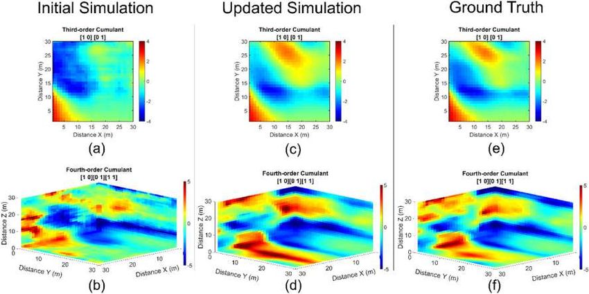
A. Kumar and R. Dimitrakopoulos Computers and Geosciences 158 (2022) 104962
Fig. 4. (a) Actor and (b) Critic agent configuration in the proposed AI algorithm.
Fig. 5. Actor and critic agents training in the proposed AI algorithm.
mineral deposits with incoming new information in an operating mining data, qi , NIi (qi ), ∀i ∈ T , along with the tracking sensor data, Track, and
environment. The spatial sensor data, NIi (x), i ∈ S , and temporal sensor initial simulations, s ∈ SI , are fed to the AI algorithm as shown in Fig. 6.
The AI algorithm then initializes the environment presented in Sect.
2.3.1 with all the information. A random path is then defined by the
environment to visit all the blocks within the mineral deposit. At each
block, a state generated by the environment is fed to the trained actor
agent that predict the updated simulated property of the block. The
environment uses the action to generate the next state, and the process
continues until all the blocks are visited. The updated simulated prop
erty of all the blocks forms the set of updated simulations SU . The
updated simulations are then used to generate the updated model-based
predictions. In parallel, the agent’s parameters are updated by training
over the updated simulations and newly collected information.
3. Application at a synthetic copper mining operation
The proposed AI algorithm is programmed using Python and Ten
sorflow. It is applied in this section to a fully known public dataset (Mao
and Journel, 1999b), which is adopted to represent a copper deposit in
the present case study. Twenty initial simulations of copper grades are
generated for two different areas, Area 1 and Area 2, of the copper de
posit using high-order simulation (Minniakhmetov et al., 2018; Yao
et al., 2018). The two areas contain 416 drillhole data points each,
sampled from the corresponding areas of the fully known dataset, with
an average spacing of 5m using random stratified sampling. Each area of
Fig. 6. Real-time learning and updating with incoming new spatial and tem the deposit consists of 13,000 blocks of size 1 x 1 x 1 m3 . The incoming
poral information.
7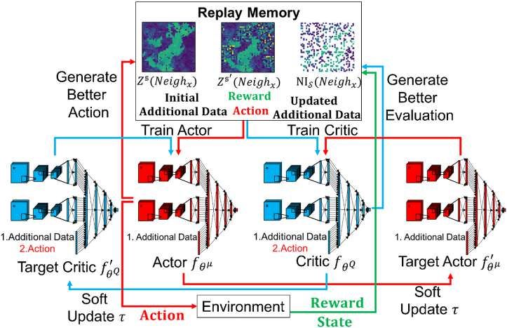
A. Kumar and R. Dimitrakopoulos Computers and Geosciences 158 (2022) 104962
spatial sensor data of copper grades is generated by randomly sampling 3.1. Parameters
2,600 data points with an average spacing of 1.3 m from the same sec
tions of the fully known dataset. The error in each spatial sensor data The proposed AI algorithm is trained on an Intel® i7-8700 machine
point is sampled from a normal distribution with a mean of 0 and a with an 8-core processor and an NVIDIA GeForce GTX 1050 GPU for
standard deviation of 0.45. The temporal sensor data of copper grades approximately 2 days. The parameters used for the case study at the
from the processing mill is generated by randomly sampling the same copper mining operation is detailed in Table 3.
section of the fully known dataset in such a way that it imitates the The actor and critic agent architecture are shown in Fig. 8. The total
process of collection of such data in a mining operation. The generated number of parameters for the actor agent is ≈ 497000, and the critic
temporal sensor data contains 2,600 data points. The error in each agent is ≈ 498000.
temporal sensor data point is sampled from a normal distribution with a
mean of 0 and a standard deviation of 0.6. The standard deviation of the 3.2. Results
normal distribution for error in the temporal sensor data is lower than in
the spatial sensor data to reflect the quality of the respective sensors. In The results described in this section for Area 1 of the deposit are
actual mining environments these sensors will show proportional effect related to the training of the agents in the proposed algorithm and shows
in their related measurement errors, however, for simplicity in demon its learning capabilities. The results for Area 2 of the deposit are related
strating the applied aspects of the proposed method proportional effect to testing of the agent and shows the generalization and applicability of
is not considered in this synthetic case study. the proposed algorithm.
The copper mining operation considered is shown in Fig. 7, and Fig. 9 and Fig. 10 show the drillhole data and two of the initial
consists of a mine, a waste dump, a processing mill and a customer. simulations of copper grade for Areas 1 and 2 of the deposit, respec
Multiple drilling machines located at the mine perform the drilling op tively. The initial simulations for Area 2 in Fig. 10 show a presence of
erations and capture the spatial new information about the grade of the very different geological patterns compared to Area 1: the curvilinear
drilled mining blocks. The materials from the mine are extracted by two structures are horizontal instead of vertical in Fig. 9. Fig. 11(a–c) and
shovels and are loaded into trucks that haul the materials to either a Fig. 12(a–c) show the spatial sensor data, the error in the spatial sensor
processing mill or a waste dump. The processing mill blends and pro data and the processing mill sensor data, respectively, that are collected
cesses the received materials to generate copper products, which are during operations in Areas 1 and 2 of the deposit, respectively.
transported to the customers. The sensors at the processing mill capture Fig. 13(a–b) and Fig. 14(a–b) show one of the initial simulations and
the temporal new information by measuring the grade of the generated its corresponding updated simulation of copper grades, respectively, for
copper products.
Two different datasets – training and testing – are generated using
Table 3
the process outlined above to represent the operations and the collection
Parameters used for the case study at the copper mining operation.
of new information in two areas, namely Area 1 and Area 2, of the de
Parameters Value
posit. The data from Area 1 of the deposit is used to train the proposed AI
algorithm. In an operating mine, this dataset would be the historical Neighx 21 x 21
data. The training results shows the learning capabilities of the proposed SI 20
algorithm. The data from Area 2 of the deposit is used for testing the Ns 8, ∀s ∈ SI
proposed algorithm. This dataset was never used for training and rep γs 10, ∀s ∈ SI
resents how the proposed algorithm would be used in an operating mine N t Ornstein-Uhlenbeck method, with a standard deviation of 1e-1 (
to update the simulations of pertinent properties of the deposit with Uhlenbeck and Ornstein, 1930).
incoming new information. Section 3.2 discusses the training and testing W 10
results of the proposed algorithm and shows that the algorithm can be τ 1e-3
generalized and has practical applications in an operating mine. NBS 500
Throughout the presentation and discussion of the results, the fully γ 0.99
known data and its histogram, variogram and spatial cumulant (Dimi NR 1e6
trakopoulos et al., 2010; Mustapha and Dimitrakopoulos, 2011) maps NI 65000
are also shown for reference. The fully known data is referred to here γMP
i
10, ∀i ∈ T
after as the ground truth model. The algorithm takes less than 30 s to c 1e-3
update the simulations of copper grade of the different areas of the NU 0, No training was performed over testing data
deposit. NTE 100
NT 200
NUE 0, No training was performed over testing data
Fig. 7. The copper mining operation.
8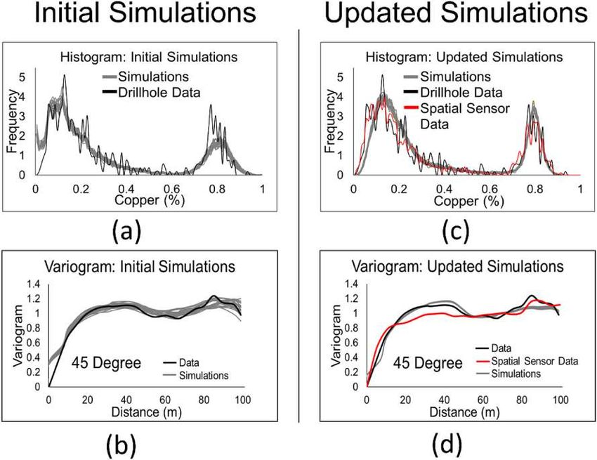
A. Kumar and R. Dimitrakopoulos Computers and Geosciences 158 (2022) 104962
Fig. 8. Actor and critic agent architecture used for the case study at the copper mining operation.
Fig. 9. Drillhole data and the 2 of the initial copper grade simulations for Area 1 of the deposit.
Fig. 10. Drillhole data and two of the initial simulations of copper grade for Area 2 of the deposit.
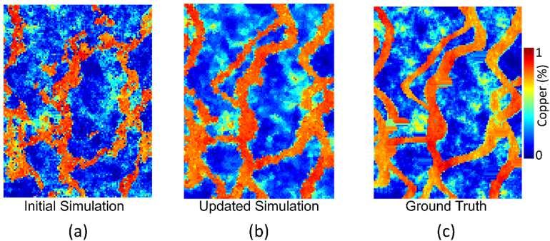
Areas 1 and 2 of the deposit. The updated simulation as shown in Fig. 13 initial simulation, and the spatial sensor data for this area, even though
(b) during training of the agents reproduces the curvilinear vertical the training data set had vertical curvilinear structures. In addition, the
structures, as inferred from initial simulations and spatial sensor data for updated simulation closely resembles the ground truth model shown in
this area. The proposed AI algorithm can also reproduce the horizontal Figs. 13(c) and Figure 14(c) for Area 1 and 2, respectively.
curvilinear structures in the updated simulation, as inferred from the The initial and updated simulations are validated through the
9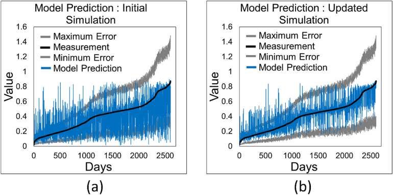
A. Kumar and R. Dimitrakopoulos Computers and Geosciences 158 (2022) 104962
Fig. 11. (a) Spatial sensor data; (b) error in the spatial sensor data; and (c) processing mill sensor data of copper grades from Area 1 of the deposit.
Fig. 12. (a) Spatial sensor data; (b) error in the spatial sensor data; and (c) processing mill sensor data of copper grades from Area 2 of the deposit.
Fig. 13. (a) One of the initial simulations compared to (b) its corresponding updated simulation, and (c) the ground truth model of copper grades for Area 1 of
the deposit.
analysis of the histogram and variogram reproduction in Fig. 15. The and 4th order spatial cumulant maps (Dimitrakopoulos et al., 2010;
initial and updated simulations both respect the histogram and vario Mustapha and Dimitrakopoulos et al., 2011), respectively, for the initial
gram of the drillhole data. The updated simulations present a closer copper grade simulation for Area 2 of the deposit. The spatial cumulant
resemblance to the histogram and variogram of the spatial sensor data, maps of the updated simulation (Fig. 16(c–d)) show more connected
as shown in Fig. 15(c) and (d), respectively. Fig. 16(a–b) show the 3rd structures, as seen in the spatial cumulant maps of the ground truth
10A. Kumar and R. Dimitrakopoulos Computers and Geosciences 158 (2022) 104962
Fig. 14. (a) One of the initial simulations compared to (b) its corresponding updated simulation, and (c) the ground truth model of copper grades for Area 2 of
the deposit.
Fig. 15. Histogram and variogram of (a–b) the initial simulations compared to (c–d) the updated simulations of copper grades for Area 2 of the deposit.
model (Fig. 16(e–f)). The proposed AI algorithm was not trained with simulation both for Area 1 and Area 2. A spread reduction (SR) criterion
data from this area, yet it still reproduces the histogram, variogram and defined by Eq. 22
spatial cumulant maps, while also updating the initial simulations of
1 ∑ 1 ∑⃒⃒ s ⃒ ⃒ ⃒
(22)
′
copper grades for Area 2 of the deposit. The histogram, variogram, and
′
SR = ⃒ I ⃒ MPi − NIi ⃒ − ⃒MPsi − NIi ⃒ , ∀ s ∈ SU
⃒S ⃒ I |T |
cumulant maps validation results for Area 1 is provided in the supple s∈S i∈T
mentary materials.
Fig. 17(a–b) and Fig. 18(a–b) show the model-based prediction for is used to quantify the reduction in measurement vs predicted values
the initial and its corresponding updated simulation of copper grades, error, for updated and initial simulations. The spread reduction value for
respectively, for Areas 1 and 2 of the deposit. The model-based predic Areas 1 and 2 of the deposit are 0.07 and 0.05, respectively, given the
tion for the updated simulation shows fewer deviations from the pro method proposed in this work.
cessing mill sensor measurements, when compared to the initial
11A. Kumar and R. Dimitrakopoulos Computers and Geosciences 158 (2022) 104962
Fig. 16. Third- and fourth-order spatial cumulant maps for (a–b) the initial simulations compared to (c–d) its corresponding updated simulations and (e–f) the
ground truth model of copper grades for Area 2 of the deposit.
Fig. 17. Model-based prediction generated with (a) an initial simulation compared to (b) its corresponding updated simulation of copper grades for Area 1 of
the deposit.
4. Conclusions proposed algorithm at a synthetic copper mining operation demon
strates its efficiency and applied aspects. The case study shows that the
This paper proposes a new self-learning artificial intelligence algo algorithm can account for softness in the incoming new information
rithm that uses deep policy gradient reinforcement learning and lever (both spatial and temporal) to update the copper grade simulations of
ages high-order spatial statistics to train actor and critic agents to update the deposit while reproducing geological patterns and high-order spatial
the simulations of pertinent spatial properties of a mineral deposit with statistics. The case study also highlights the learning and generalization
incoming new information. The algorithm is general and can be applied capabilities of the algorithm through its application in different parts of
to any mining operation with multiple sources of incoming new infor the deposit, which have different geological patterns and curvilinear
mation. The algorithm visits the mining blocks within the deposit structures. The algorithm proposed in this work is not limited to the
following a random path. For each block, a state representation is number of mining blocks used during training, however, the updating
generated and fed to the actor and critic agent, in this case a convolu time during testing will increase as the number of blocks that need to be
tional neural network. The actor agent takes an action, which is to updated increases. The proposed algorithm assumes that the training
predict the updated spatial properties of the blocks based on the state and testing areas present similar geological characteristics. The exten
representation. The action is evaluated by the critic agent. In parallel, sion of the proposed algorithm to 3-dimensional deposits is straight
the environment also evaluates the action using high-order spatial sta forward by using convolution 3D layers in the agent’s architecture.
tistics and generates both a reward and the next state representation. Future research will focus on expanding and applying the algorithm for
The state, action, reward and next state data is stored in a replay multiple elements and using preferentially sampled new incoming in
memory, which is sampled at regular intervals to train the agents. The formation from an operating mine.
improved agents are then used for further training. An application of the
12A. Kumar and R. Dimitrakopoulos Computers and Geosciences 158 (2022) 104962
Fig. 18. Model-based prediction generated with (a) an initial simulation compared to (b) its corresponding updated simulation of copper grades for Area 2 of
the deposit.
CRediT authorship contribution statement References
Ashish Kumar: Conceptualization, Methodology, Software, Data Aanonsen, S., Nævdal, G., Oliver, D., Reynolds, A., Vallès, B., 2009. The ensemble
Kalman Filter in reservoir engineering: a Review. SPE J. 14, 393–412.
Preperation, Visualization, Validation, Writing – original draft, Writing Ángel, P., Benndorf, J., Mueller, U., 2021. Resource and grade control model updating
– review & editing. Roussos Dimitrakopoulos: Supervision, Writing – for underground mining production settings. Math. Geosci. 53, 757–779. https://doi.
review & editing, Funding acquisition. org/10.1007/s11004-020-09881-2.
Benndorf, J., 2020. Data assimilation for resource model updating. In: SpringerBriefs in
Applied Sciences and Technology. Springer, pp. 19–60. https://doi.org/10.1007/
978-3-030-40900-5_3.
Declaration of competing interest Benndorf, J., 2015. Making use of online production data: sequential updating of mineral
resource models. Math. Geosci. 47, 547–563. https://doi.org/10.1007/s11004-014-
9561-y.
The authors declare that they have no known competing financial Chaowasakoo, P., Leelasukseree, C., Wongsurawat, W., 2014. Introducing GPS in fleet
interests or personal relationships that could have appeared to influence management of a mine: impact on hauling cycle time and hauling capacity. Int. J.
the work reported in this paper. Technol. Intell. Plann. 10, 49–66. https://doi.org/10.1504/IJTIP.2014.066711.
Chen, Y., Oliver, D.S., 2012. Ensemble randomized maximum likelihood method as an
iterative ensemble smoother. Math. Geosci. 44, 1–26. https://doi.org/10.1007/
Acknowledgement s11004-011-9376-z.
Conjard, M., Grana, D., 2021. Ensemble-based seismic and production data assimilation
using selection kalman model. Math. Geosci. 1–24 https://doi.org/10.1007/s11004-
The work in this paper was funded by the National Sciences and 021-09940-2.
Engineering Research Council (NSERC) of Canada CRD Grant 500414- Dalm, M., Buxton, M.W.N., van Ruitenbeek, F.J.A., 2018. Ore–waste discrimination in
epithermal deposits using near-infrared to short-wavelength infrared (NIR-SWIR)
16 and NSERC Discovery Grant 239019, the industry consortium
hyperspectral imagery. Math. Geosci. 51, 1–27. https://doi.org/10.1007/s11004-
members of McGill University’s COSMO Stochastic Mine Planning 018-9758-6.
Laboratory (AngloGold Ashanti, Barrick Gold, BHP, De Beers, IAM De Jong, T.P.R., 2004. Automatic sorting of minerals. In: IFAC Proceedings, pp. 441–446.
GOLD, Kinross Gold, Newmont Corporation, and Vale); and the Canada https://doi.org/10.1016/s1474-6670(17)31064-9.
Deutsch, C., Journel, A.G., 1992. In: GSLIB: Geostatistical Software Library and User’s
Research Chairs Program. Guide, second ed. Oxford University Press, New York.
Dimitrakopoulos, R., Mustapha, H., Gloaguen, E., 2010. High-order statistics of spatial
random fields: exploring spatial cumulants for modeling complex non-Gaussian and
Appendix A. Supplementary data non-linear phenomena. Math. Geosci. 42, 65–99. https://doi.org/10.1007/s11004-
009-9258-9.
Supplementary data to this article can be found online at https://doi. Fu, J., Gómez-Hernández, J.J., Du, S., 2017. A gradient-based blocking Markov chain
Monte Carlo method for stochastic inverse modeling. In: Quantitative Geology and
org/10.1016/j.cageo.2021.104962. Geostatistics. Springer, Cham, pp. 777–788. https://doi.org/10.1007/978-3-319-
46819-8_53.
Gilman, J., Ozgen, C., 2013. Reservoir Simulation: History Matching and Forecasting.
Computer code availability
Society of Petroleum Engineers, Texas.
Goetz, A.F.H., Curtiss, B., Shiley, D.A., 2009. Rapid gangue mineral concentration
• Name of code: MineralDepositAI measurement over conveyors by NIR reflectance spectroscopy. Miner. Eng. 22,
• Developer: Ashish Kumar (McGill University, FDA Building, Quebec, 490–499. https://doi.org/10.1016/j.mineng.2008.12.013.
Gómez-Hernández, J.J., Srivastava, R.M., 2021. One step at a time: the origins of
Canada; ashish.kumar@mail.mcgill.ca) sequential simulation and beyond. Math. Geosci. 53, 193–209. https://doi.org/
• Year first available: 2020 10.1007/s11004-021-09926-0.
• Hardware required: Windows with NVIDIA GPU of at least 4 GB Gutiérrez-Esparza, J.C., Gómez-Hernández, J.J., 2017. Inverse modeling aided by the
classification and regression tree (CART) algorithm. In: Quantitative Geology and
memory and compute capability of 6 and higher Geostatistics. Springer, Cham, pp. 805–819. https://doi.org/10.1007/978-3-319-
• Software required: Python Integrate Development Environment 46819-8_55.
(Visual Studio, 2015 preferred) Hu, L.Y., 2000. Gradual deformation and iterative calibration of Gaussian-related
stochastic models. Math. Geol. 32, 87–108. https://doi.org/10.1023/A:
• Program language: Python 3.6.1 1007506918588.
• Program size: 85.8 MB (including source code, documentation, re Iyakwari, S., Glass, H.J., Rollinson, G.K., Kowalczuk, P.B., 2016. Application of near
sults, and data) infrared sensors to preconcentration of hydrothermally-formed copper ore. Miner.
Eng. 85, 148–167. https://doi.org/10.1016/j.mineng.2015.10.020.
• Access to code: download from https://github.com/ashishrokz1993
/MineralDepositAICG
13You can also read