COLORADO 2050: WHY WE NEED CLIMATE RESILIENCY TO PROTECT OUR COMMUNITIES AND WAY OF LIFE
←
→
Page content transcription
If your browser does not render page correctly, please read the page content below
COLORADO 2050:
WHY WE NEED CLIMATE
RESILIENCY TO PROTECT OUR
COMMUNITIES AND WAY OF LIFE

                              1
INTRODUCTION
    Climate change is creating challenges for Colorado in
    many ways. We are already seeing its effects in the form                                           METHODOLOGY
    of increased temperatures, lower snowpack, severe
    drought, and extreme wildfires. These phenomena              In this study, we first ranked census tracts based on their
    impose economic damage on the state, put the physical        exposure to four climate change impacts: extreme heat,
    and mental health of Coloradans at risk, threaten biodi-     air pollution, wildfires, and drought. We used climate
    versity, and can destabilize ecosystems.                     change projections under two emission scenarios:
                                                                 moderate-emission (RCP 4.5) and high-emission
    The goal of this research is to identify Colorado commu-     (RCP 8.5) by mid-century (2050). We defined a
    nities most at risk of the negative effects of climate       social vulnerability index, which takes into account
    change and guide policymakers on potential climate           demographic, socioeconomic, and health indicators
    mitigation investments and effective response strategies     in each tract. This index is a number between 0 and
    to build resilient communities in every part of the state.   1, which ranks tracts with respect to one another and
                                                                 provides a measure of relative vulnerability of different
    The study consists of two sections:                          geographic areas. 0 is the lowest vulnerability and 1 is
                                                                 the highest vulnerability. We used a modified version
    1.   Exposure to climate change impacts:                     of the Centers for Disease Control’s social vulnerability
         This report focuses on four impact of climate change    index (SVI) to make it more relevant to climate change,
         in different areas of the state:                        combining 16 parameters into one index. Finally, we
            a.       Heat                                        overlayed the climate and social exposure to find tracts
            b.       Ozone                                       that are at higher risk of climate change impacts.
            c.       Wildfires
            d.       Drought                                        waves. Workers who do their jobs outdoors are also
                                                                    more exposed to the extreme effects of climate
    2.   The need for resiliency:                                   change and might have higher financial vulnerability
         Climate change imposes higher costs to commu-              as these types of effects worsen.
         nities with the most barriers to socioeconomic
         success. Low-wage workers, communities of color,
         people with lower levels of educational attainment,     People in these demographic, socioeconomic, and
         and linguistically isolated groups usually live in      health-related categories are at the highest risk of
         more polluted areas, have fewer resources, and less     being exposed to threats posed by climate change. By
         mobility. People with pre-existing health conditions    studying the data, we can find which communities are
         — like asthma or heart disease — are vulnerable to      at the highest risk of each climate threat. Identifying
         the health impacts of air pollution and the youngest    the communities most affected by climate impacts is
         and oldest Coloradans are more susceptible to the       essential for policymakers as they make decisions about
         health effects of extreme weather events like heat      climate adaptation and mitigation.
2
CLIMATE EXPOSURE                                                                                                      DEFINITION
Greenhouse gas (GHG) emissions from human activities                          IPCC defines exposure as “the presence of people,
have raised global average temperatures significantly                         livelihoods, species or ecosystems, environmental
during the past 100 years (IPCC, 2013). As global tempera-                    functions, services, and resources, infrastructure,
tures continue to rise, Colorado will be increasingly                         or economic, social, or cultural assets in places and
exposed to the impacts of climate change. In this study,                      settings that could be adversely affected. Exposure is an
we analyze Colorado’s projected exposure to extreme                           important precondition for considering a vulnerability
heat, drought, wildfires, and air pollution.                                  as key. If a community is not exposed to a certain
                                                                              climate impact, their vulnerability to that impact will be
Extreme Heat: Regions of Colorado have experienced                            irrelevant ”(Oppenheimer et al., 2015).
between 0.5 degrees to more than 3 degrees Fahrenheit
of warming between 1986–2016 compared to 1901–1960
(Vose et al., 2017). All climate models project that
Colorado’s climate will warm substantially by 2050 (Lukas                     Drought: Over the past 30 years, soil moisture drought
et al., 2014). This warming will drive longer, hotter, and                    has become more severe in Colorado (Lukas et al.,
more intense heat waves which increase the risk of heat                       2014). Drought affects crop yield, water supply, and the
stroke and other illnesses that can cause premature                           recreation industry in Colorado. Moreover, as demand
deaths. Young people, older people, people with existing                      for water increases with the growth of our state’s
health conditions, and those who work outdoors are                            population, the agriculture industry and Colorado’s food
affected most by rising temperatures (Hughes and                              security will be threatened. Warm and dry conditions
Fenwick, 2016).                                                               have also prolonged periods of bark beetle survival and
                                                                              reproduction, reducing the resistance of trees to beetle
Ozone Pollution: Ground-level ozone is formed                                 attacks and increasing tree mortality (Raffa et al. 2008).
primarily from reactions between two major classes of                         Tree mortality affects snow accumulation, snowmelt, and
air pollutants: volatile organic compounds (VOCs) and                         water uptake by vegetation (Lukas et al., 2014), affects
nitrogen oxides (NOx).1 Sunlight and heat accelerate                          water quality (Gonzalez et al., 2018) and makes the forest
these reactions, so high concentrations of ozone usually                      more susceptible to surface fires (Stephens et al., 2018).
occur during summer months. Ground-level ozone can
have adverse health effects such as premature death
(Nuvolone and Voller, 2018), respiratory and cardiovas-
cular problems (WHO, 2013), and aggravated asthma
(Fann et al., 2016). In Colorado, the Denver Metro Area
as well as some parts of Boulder and Weld counties
have significantly higher ozone concentrations due to
their proximity to highways, traffic, and other sources
of pollution such as refineries and factories. Climate
change can exacerbate ozone pollution because rising
temperatures facilitate formation of ozone molecules.

Wildfire: Climate change has also increased the
intensity, extent, and duration of wildfire season, partic-
ularly due to prolonged dry conditions and reduced
soil moisture (Littell et al., 2016, Chikamoto et al., 2017).
Wildfire suppressions in the past century and land
management policies have also promoted biomass
accumulations which have contributed to frequent
large wildfires—events that were rare under natural fire
regimes (Allen et al., 2002). Three of the largest fires in
Colorado occurred in 2020, with the total area of 541,482
acres burned2. An increasingly high number of homes
in wildland urban interface3 areas have also elevated
wildland fire to a growing public safety concern, causing
catastrophic damage in the last two decades.4

1. https://www.epa.gov/ozone-pollution-and-your-patients-health/what-ozone
2. Wildfire News & Information | Fire Prevention and Control
( https://www.colorado.gov/pacific/dfpc/wildfire-news-information )
3. The wildland-urban interface is any area where man-made improvements are
built close to, or within, natural terrain and flammable vegetation.
4. https://cdpsdocs.state.co.us/dfpc/WebsitePhotos/Playbook.pdf
                                                                                                                                           3
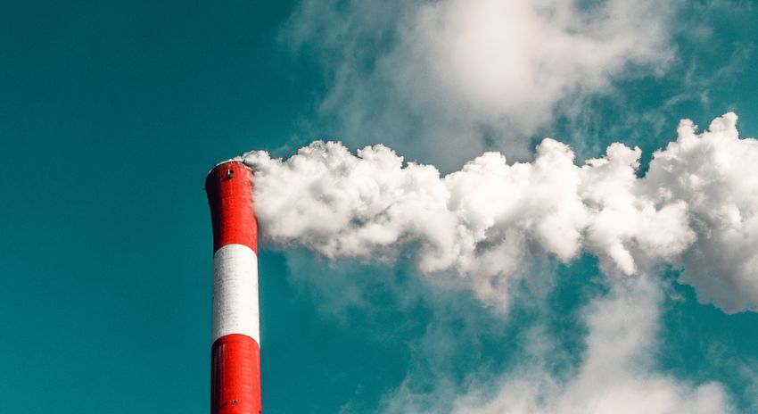
Climate change scenarios
    The Intergovernmental Panel on Climate Change (IPCC)
    has developed possible scenarios to show trajectories of
    future climates based on different levels of GHG concen-
    trations. These trajectories are called Representative
    Concentration Pathways (RCPs) and represent possible
    “radiative forcing values”5 that would result from green-
    house gases in the atmosphere in 2100. As shown in
    Figure 1, RCP 8.5 represents the high-emission scenario,
    which increases the global average temperatures by
    4.2°–8.5°F by the end of the century, relative to the
    1986–2015 average. The high emission scenario is referred
    to as a “business-as-usual” scenario, which will have the
    worst climate consequences and occurs if we continue
    burning fossil fuels at the current trend, without policies
    to curb our emissions.

    Under RCP 4.5 (moderate emission scenario), global
    average temperatures are projected to increase by
                                                                                                 Figure 1: Representative Concentration Pathways
    1.7°–4.4°F. This scenario assumes a range of technologies
    and strategies for reducing greenhouse gas emissions                                 Thick lines represent the average of multiple climate models and
    will be adopted to stabilize global temperatures before                             the shaded ranges illustrate the 5 percent to 95 percent confidence
                                                                                                         intervals. Source: Hayhoe et al., 2018
    the end of the century.

    In this study, we compare climate impacts under RCP 4.5
    and RCP 8.5 scenarios.

    5. “Radiative forcing is the change in the net, downward minus upward, radiative
    flux (expressed in Watts per square meter) at the atmosphere due to a change
    in an external driver of climate change, such as a change in the concentration of
    carbon dioxide (CO2) or the output of the Sun.” (Source: IPCC)
4
EXTREME HEAT                                                                                                  DEFINITION
                                                                   Extreme heat can be defined in different ways. We use
Extreme heat episodes disproportionately threaten                  the deviation from an average historical temperature as
the health and well-being of young people, older                   the definition of extreme heat (Cooley, 2012).
people, those with certain medical conditions, and
outdoor workers (USGCRP, 2016; Hughes and Fenwick,                 We define days with extreme heat as days when the local
2016). Since people in different areas of the state have           daily maximum temperature exceeds the 95th percentile
historically adapted to different levels of heat, there is         of local historic daily maximum temperature (1980-2010)
no fixed temperature that can capture the true extreme             between May 1 and September 30. This is the daily
heat experience at the local level. People in some areas           maximum temperature that is exceeded on 5 percent
are accustomed to temperatures above 100 degrees in                of summer days in the historic period. By definition, the
summer, while in other areas temperatures above 90                 95th percentile temperature is exceeded on 7.6 days
degrees are difficult to tolerate. Even relatively moderate        each summer (5 percent of 153 days of summer).
heat can cause heat-related illness or death for those
who are not acclimated to it (Cooley, 2012). For this              We compare future temperature projections with
reason, we define extreme heat as temperatures that are            historical temperature data to find how many days in each
hotter than 95th percentile historic maximum tempera-              scenario exceed the historic 95th percentile temperature.
tures at each census tract. This is the temperature in
each census tract that is historically exceeded on only 5          Using historic temperature data at 185 temperature
percent of summer days in the 30-year historic period.             monitoring stations, we use ordinary Kriging method to
                                                                   spatially interpolate the temperature everywhere across
                                                                   the state and predict the temperature at each census tract.

                        Figure 2: 95th percentile maximum daily temperatures 1980-2010 (degrees Fahrenheit)

                                                                                             TEMPERATURE MODELS
                                                                   For future temperature projections, we use three
Figure 2 shows the 95th percentile of historic (1980-2010)         downscaled CMIP5* models for two emission scenarios,
maximum daily temperatures by census tract. The map                RCP 4.5 (moderate emission scenario) and RCP 8.5 (high
shows a wide range of temperatures ranging from                    emission scenario) by mid-century (2045-2055). Models
70 degrees in the central and southwest mountains,                 used for projection of daily maximum temperature are
to 95 degrees in the southeast plains. For example,                bias-corrected constructed-analogs downscaled data
the temperature that has historically exceeded only 5              (BCCAv2-CMIP5-Climate-daily), with resolution of 1/8th
percent of days in Bent County is 95 degrees while in              degrees (about 8.7 miles). For each emission scenario,
Lake County, on average, temperatures have only gone               the average of three models is used (CCSM4 (USA),
above 70 degrees 5 percent of days in any given year.              MRI-CGCM3 (Japan), GDFL-GSM2G (USA)).

                                                                                                                                 5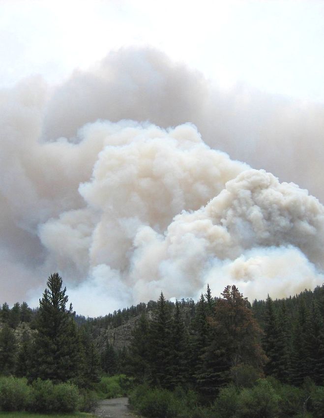
Figure 3 shows the projected number of days those                           temperatures above their local historic extreme). In the
    temperatures will exceed the historic 95th percentile by                    high emission scenario, the median is 88.6 days each
    mid-century under two emission scenarios. Under the                         summer with temperatures exceeding the local extreme.
    moderate emission scenario, northern counties as well                       Exposure to extreme temperature significantly increases
    as the Denver Metro Area are projected to experience                        mortality in all age groups, especially among older
    75 days of extreme heat on average, while under high                        people, young children, and people with certain medical
    emission scenario, average number of extreme heat                           conditions (Greene et al., 2011). Between 2011 and
    days in the same region is projected to be 100 days.                        2018, on average about 450 heat-related emergency
                                                                                department visits were made each year across the state.
    Across the state, in the moderate-emission scenario,                        Excess heat also reduces labor hours due to unsuitable
    the median number of days above the 95th percentile                         working conditions. This is especially true for high-risk
    historical is 76.5 days (so half of the census tracts                       industries where workers are doing physical labor and
    experience at least 76.5 days each summer with                              have a direct exposure to outdoor temperatures (e.g.,

           Figure 3: Average annual number of summer days exceeding the 95th percentile historic maximum daily temperature, mid-century.

                                                                a) Moderate emission scenario

                                                                 b) High emission scenario

    agriculture, construction, utilities, and manufacturing). Increases in temperature will also result in increased energy
    use for cooling and decreased energy use for heating. Rising temperatures are expected to cause a net increase in
    electricity consumption since summer cooling needs are expected to grow faster than the decline in winter heating
    needs.6
    6. https://nca2014.globalchange.gov/report/sectors/energy
6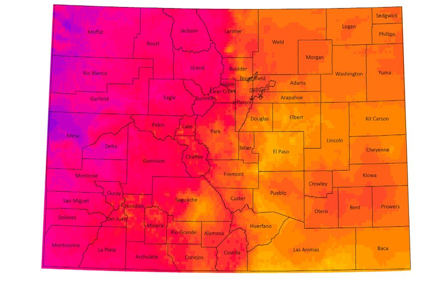
OZONE POLLUTION

Air Pollution (Ozone)
                                                                                            DEFINITION AND METHODS
The Environmental Protection Agency (EPA) has imple-                  Average daily 8-hour maximum ozone concentration
mented national standards for air pollution to protect                is the daily maximum surface ozone concentration, in
public health. Any area that does not meet the national               parts per billion (PPB), averaged over 8 hours.
primary or secondary ambient air quality standard
is classified as a “nonattainment area.” Depending                    We use results of Climate impacts simulations by
on how high the ozone pollution level is, the ozone                   Skamarock and Klemp (2008) which uses the CCSM4
nonattainment area can be categorized as marginal,                    GCM under RCP8.5 and RCP4.5 and dynamically
moderate, serious, severe, or extreme.                                downscaled over North America using the Weather
                                                                      Research and Forecasting (WRF) model.
Since 2016, the Denver Metro Area had been classified by
the EPA as a “moderate” nonattainment area for ozone                 In 2015, the EPA set the ground-level ozone standard
pollution. Under the Clean Air Act, areas that do not                to 0.070 ppm, averaged over an 8-hour period. This
attain national ozone standards in a timely manner are               standard is met at an air quality monitor when the 3-year
reclassified to a higher nonattainment status. In 2019, the          average of the annual fourth-highest daily maximum
EPA reclassified the Denver Metro/North Front Range                  8-hour average ozone concentration is less than or equal
ozone nonattainment area from “moderate” to “serious”                to 0.070 ppm. Figure 5 shows projections of average
nonattainment. A 2020 study by the American Lung                     ozone concentration levels by mid-century during
Association ranks Denver in the top 10 of their list of              summer months.
most-polluted cities in the country for ozone pollution.7
According to a 2017 study8 by the National Center for                In both scenarios, on average, ozone concentration levels
Atmospheric Research (NCAR), the major contributors to               increase by about 3 percent across the state compared
the North Front Range’s ozone pollution were emissions               to the baseline period (2000).10 Under both emission
from oil and gas operations, as well as traffic.                     scenarios, the highest increase in ozone concentration
                                                                     levels are projected to occur in the Northern Front
Climate change is expected to increase future levels of              Range, Northern Plains, and Southern Plains. Some of
ozone concentrations since there is a strong correlation             the counties in these regions (Jefferson, Douglas, Denver,
between higher ozone levels and higher temperatures.                 Adams, Arapahoe, Broomfield, Boulder) currently have
Moreover, warmer days will increase the demand for air               significantly higher ozone concentrations compared to
conditioning and electricity consumption, and electric               the rest of the state, which is caused by high proximity
power plants emit NOx,9 which is one of the components               to highways and traffic as well as refineries and other
that generate ground-level ozone.                                    factories.
7. https://www.lung.org/research/sota/key-findings/ozone-pollution
8. https://www2.acom.ucar.edu/frappe                                 10. Source for 2000 data: EPA daily air quality data
9. https://www.giss.nasa.gov/research/features/200402_tango/         ( https://www.epa.gov/outdoor-air-quality-data/download-daily-data )
                                                                                                                                            7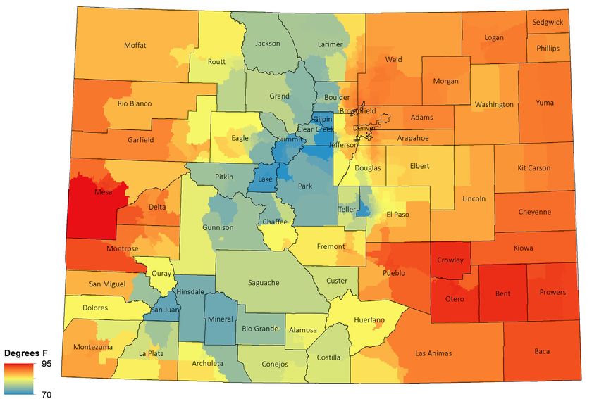
The Impact of Ozone Pollution:
    Exposure to ozone pollution can cause serious health complications, including inflammation and damage to the
    airways, and aggravated lung diseases such as asthma, emphysema, and chronic bronchitis. Exposure to air pollution
    also increases the risk of death from COVID-19 (Wu et al., 2020). Data from the Colorado Department of Public Health
    and Environment11 shows Denver, El Paso, Jefferson, Arapahoe, and Adams counties are top-five counties in deaths
    from COVID cases. These counties also have high levels of air pollution exposure.
    11. https://covid19.colorado.gov/data

                     Figure 4: Change in summer-average maximum daily 8-hour ozone concentrations (ppb) in 2050 (compared to 2000)

                                                             a) Moderate emission scenario

                                                                 b) High emission scenario

8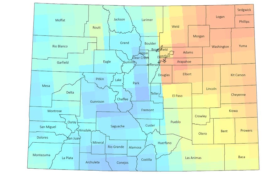
WILDFIRES

Wildfires:
Forests serve an important role in the ecosystem.
Wildlife habitat, erosion control, water filtration, and                            DEFINITION AND METHODS
recreation are all dependent on healthy forests. Climate
change increases the probability and intensity of                     Very high fire danger is defined as the average number
wildfires and increases the wildfire season duration                  of days with 100-Hour Fuel Moisture below 10th
(Abatzoglou & Williams, 2016) through increased heat,                 percentile of the baseline period (1971-2000).
long-lasting droughts, reduced soil moisture, and other
disturbances, all of which threaten the place of forests in           The 100-Hour Fuel Moisture value represents the
local ecosystems. Wildfires also have severe impacts on               modeled moisture content of dead materials on the
air quality and human health. Fire seasons are now 78                 forest floor. We use a model mean derived from 18
days longer than they were 40 years ago, and out of 161               downscaled CMIP5 models to project 100-Hour Fuel
wildfires for which the state was responsible between                 Moisture by mid-century.
1967 and 2018, 138 fires occurred after 2000.12
12     https://cdpsdocs.state.co.us/dfpc/WebsitePhotos/Playbook.pdf

                                                                                                                               9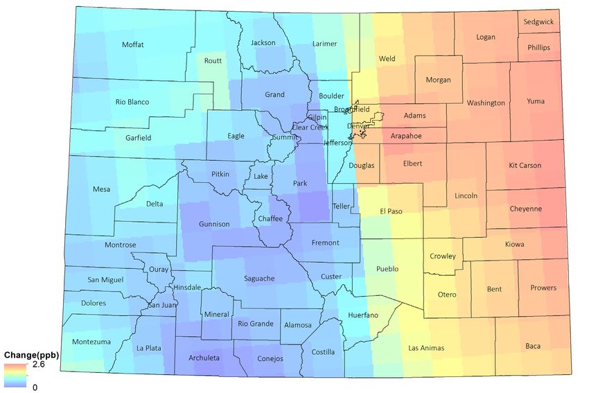
Figure 5 shows the projections of “very high fire danger” during June, July, and August by mid-century. The darker
     colors indicate a higher number of days where fire danger is very high. Western counties, especially those in the
     Grand Valley, Northern Mountains, and western San Juan Mountains regions face the highest risk, especially
     Mesa, Rio Blanco, and Moffat counties which are projected to face up to 39 days of high summer fire danger by
     mid-centurymid-century. This is about eight days higher than the historic average (1971-2000) for this area. Prowers,
     Bent, and Otero counties have fewer projected days with very high fire danger (23 to 25 days), but the change from
     historic values is higher (they are projected to experience 9-10 extra days with very high fire danger compared to the
     baseline period).

                                   Figure 5: Very high fire danger, mid-century. Source: climatetoolbox.org

                                                        a) Moderate emission scenario

                                                         b) High emission scenario

10
Figure 6: Cost of Wildfires and Acres Burned.
Billion-Dollar Weather and Climate Disasters: Time Series | National Centers for Environmental Information
Between January 2000 and October 2020, Colorado past five decades. The figure shows that costs of wildfires
suffered total statewide wildfire-related damages to have significantly increased during the past decade.
property and crops of about $1.8 billion, as well as seven Estimated costs include physical damage to residential,
deaths and 17 injuries.13 More than $295 million of these commercial, and government or municipal buildings;
damages and three of the largest wildfires in Colorado material assets within a building; time element losses
happened in 2020 (Cameron peak, 208,663 Acres; East like business interruption; damage to vehicles and
Troublesome, 193,812 Acres; and Pine Gulch, 139,007 boats; offshore energy platforms; public infrastructure
Acres).14 The cost of wildland fire suppression in Colorado like roads, bridges, and buildings; agricultural assets
has grown significantly with the increased occurrence like crops, livestock, and timber; disaster restoration and
of large fires. Figure 6 shows the National Oceanic and wildfire suppression costs. Climate change is projected
Atmospheric Administration’s estimate of the area to increase the number and frequency of such large
burned by wildfires and their estimated cost over the wildfires.
13. https://www.ncdc.noaa.gov/stormevents/
14. https://www.colorado.gov/pacific/dfpc/wildfire-news-information
11DROUGHT
According to the Colorado Climate Center, Colorado
endured five significant dry periods prior to 2000:
1893-1905, 1931-1941, 1951-1957, 1963-1965, and 1975-1978.
Since the turn of the century, Colorado has experienced DEFINITION AND METHODS
several years of severe drought with 2002, 2012, 2018, and
2020 being some of the driest on record. Drought is defined as shortage of water that occurs
due to lack of precipitation such as rain, snow, or sleet
The 2020 drought ranks as the second-worst drought in for a prolonged period of time. Even though droughts
the last 20 years across Colorado. It was also the fourth occur naturally, human activity, such as water use and
time in two decades – following 2002, 2006 and 2012 management can exacerbate dry conditions.
– that 100 percent of Colorado was categorized as abnor-
mally dry or in various degrees of drought. By November
2020, 27 percent of the state, mostly in Western
Colorado, was in “exceptional” drought condition.
Climate change exacerbates drought conditions in many
areas of the United States, especially in the Southwest.
In Colorado, water and snow-based recreation
industries, agriculture, and fish and wildlife population
are negatively impacted by drought. Drought can
exacerbate fire season since dry vegetation provides fuel
and fire can spread easily over dry soil.
Soil moisture
Rising temperatures increase the water evaporation rate
from soil and plants and can make the soil drier. During
the last few decades, soil became drier in most of the
state, especially in the summer (EPA, 2016). In future
decades, summer precipitation and runoff are likely to
decrease in Colorado and droughts are likely to become
more frequent and more severe (Averyt et al., 2011).
Dryland crops are entirely dependent on precipitation
and are more susceptible to damage from drought.
Dryland crops are particularly vulnerable to severe
“single-season” droughts that deplete soil moisture
(CWC, 2013). Wheat, corn, sorghum, hay, proso millet, and
sunflowers are the most extensively grown dryland crops
in Colorado.
12Figure 7 shows the area of farmland as a percentage of the total area of each county. Dark red
areas indicate counties with more than 90 percent farmland. The figure shows that eastern
counties are more heavily dependent on agriculture and farming compared to the rest of
the state. Logan, Sedgwick, Phillips, Kit Carson, and Prowers counties are over 95 percent
farmland, meaning drought has significant impacts on the economy in these counties.
Figure 8 shows the percentage of agriculture jobs by county. In Kiowa, Cheyenne, Sedgwick,
Washington, and Baca counties, more than 40 percent of all jobs are in the agriculture sector,
with Kiowa having the highest agricultural employment (76 percent). These counties are at
higher risk of economic loss in times of drought.
Figure 7: Farmland (percent total area), 2017
Figure 8: Jobs in Agriculture sector (% employed population over 16 yo), 2019
State Demography Office
13We use projections of precipitation anomaly as a proxy for
soil moisture that impacts agriculture in Colorado. To find
METHODS
the anomaly, we compared future projections of precipi- We used average of precipitation projections from three
tation with historic average precipitation. Figure 9 shows climate models: CCSM4 (USA), MRI-CGCM3 (Japan), and
normal precipitation as an annual average over 30 years GDFL-GSM2G (USA), and interpolated the projections
(1980-2010) and Figure 10 shows the change in precipi- across the state using ordinary Kriging method to find
tation by mid-century under the high emission scenario. precipitation change at each census tract.
Figure 9: Average annual 30-year (1980-2010) Precipitation (mm)
Figure 10: Percent Change from average annual 30-year (1980-2010), mid-century, high emission scenario
Figure 10 shows that the highest decrease in precipitation is projected to occur in the Central Mountains and
Western San Juan Mountains regions, where rain and snowfall will decrease by as much as 62 percent. While some
counties in the Southern Plains region, especially Bent, Crowley, Otero, Kiowa, and Lincoln, as well as some areas in
the Southern Front Range region (Pueblo, El Paso, Fremont) are in fact projected to experience significant increases
in precipitation, the model does not distinguish between snow and rainfall. Climate change can shift precipitation
from snow to rain and increase the frequency of heavy rainfall. It is estimated that heavy rain has increased in
Colorado by 5 percent between 1958 and 2012.15 An increase in heavy rainfall will increase the risk of flooding, which
can destroy homes, roads, and crops. A recent example is the 2013 flood in Northern Colorado, where we received
almost a year’s worth of rainfall (17 inches) in four days.
15. https://nca2014.globalchange.gov/report/our-changing-climate/heavy-downpours-increasing#graphic-16693
14METHODS
“The analysis uses the Utah
Energy Balance (UEB) model,
a water and energy balance
model which tracks snow-water
equivalent (SWE), internal energy
of the snowpack, and snow
surface age in its simulation
of snow accumulation and
Figure 11: Change in ski season length (#days) compared to baseline (1986-2005) melt. The model simulates
a) Moderate emission scenario natural snow accumulation
and snowmelt at the winter
recreation sites using site-specific
climatic and topographic
characteristics of each site. At
each of the modeled locations,
results include a simulation of
natural snowpack for the 20-year
reference period (1986-2005),
and future simulations for the
20-year periods centered on
the reporting years of 2050 and
2090 for each of five GCMs under
RCP8.5 and RCP4.5.” (EPA, 2017)
b) High emission scenario
Tourism is a major economic driver for Colorado, contrib- economic losses (Williamson et al., 2008). Figure
uting greatly to the state’s revenue and employment. 12 shows the average change in ski season length
In 2016, the hospitality industry was Colorado’s second- (average of change in cross country skiing season
largest employer, employing 165,000 workers and about length and Nordic skiing season length). Blue circles
generating about $5 billion in economic activity. Climate show the decrease in season length in days at the 19
change threatens Colorado’s winter tourism as rising locations compared to a 1986-2005 baseline. Bigger
temperatures will lead to less snow. The IPCC predicts circles indicate a larger decrease in the season length.
that a 1.8° F increase in annual global temperatures Figures show that under the high emission scenario,
will decrease snowpack by 20 percent in the Northern climate change will shorten ski season at some resorts
Hemisphere (IPCC 2007). Diminishing snowpack by as many as 65 days. Even in the moderate emission
will shorten the ski season and skiing in Colorado scenario, the season length could decrease by as
will become less reliable, leading to climate-related many as 53 days (Routt County).
15BARRIERS TO
RESILIENCY
Individuals and communities are different in their access
to resources to prepare for, cope with, and recover from DEFINITION
hazardous events such as natural disasters, disease
outbreak, or anthropogenic pollution. Socioeconomic IPCC defines vulnerability as “the propensity or
status, health, and demographic factors can impact the predisposition to be adversely affected. Vulnerability
preparedness and resilience of communities in the face encompasses a variety of concepts and elements
of natural disasters and climate change impacts (Adger, including sensitivity or susceptibility to harm and lack of
1999; Otto et al., 2017). capacity to cope and adapt.” (Oppenheimer et al., 2015).
For most of the 20th century, disaster management
focused on physical infrastructure. In the 1970s,
researchers realized the importance of socioeconomic
factors that affected community resilience (Juntunen,
2004). In mitigating and planning for emergencies, state,
local, and tribal officials must identify the communities
with barriers created by structural inequality and
disinvestment in order to serve those residents over the
course of a disaster.
As we saw in the previous section, climate change will
exacerbate exposure to environmental hazards. Climate
change is also expected to exacerbate existing barriers
and inequalities, which in turn will deepen intergen-
erational inequity by creating even more barriers for
communities to overcome in order to access natural and
financial resources (Otto et al., 2017).
To determine the ability for Colorado communities to be
resilient to climate change, we used a modified version
of the Centers for Disease Control and Prevention’s
“social vulnerability” index (SVI) that takes into account
a combination of demographic, socioeconomic, and
health variables. The SVI indicates the relative threat to
every U.S. Census tract. “The SVI is intended to spatially
identify [these] populations, to help more completely
understand the risk of hazards to these populations, and
to aid in mitigating, preparing for, responding to, and
recovering from that risk” (Flanagan et al., 2011).
16To calculate the social vulnerability index, we use the methodology used by CDC to calculate the SVI: For each census
tract, we generated its percentile rank among all tracts for each individual variable, as well as its overall position. For
overall tract rankings we summed the percentiles, and then calculated overall percentile rankings.
Before ranking, we adjusted the cardinality to ensure that the sign of the factor reflects its contribution to vulnerability.
For example, a high percentage of linguistically isolated residents indicate higher vulnerability, giving this variable a
cardinality of +1, while higher income indicates lower vulnerability, and receives cardinality of -1.
We should keep in mind that the SVI has certain limitations. First, it compares census tracts based on where people
live, not necessarily where they work or play. Second, the composition of some smaller census tracts might change
rapidly, and the geographic boundaries of census tracts can change based on changes in population. Finally, SVI does
not take into account the vulnerability of the physical infrastructure and community assets or other resources that
may help to reduce the effects of the hazard.
The parameters used in our analysis are: METHODS
Economic:
• Poverty (percentage of people below federal poverty line (2014-18 ACS))
• Unemployment (percentage, civilian noninstitutionalized (2014-18 ACS))
• PCI (Per capita income (2014-18 ACS))
• Home ownership (% Renter-occupied, Occupied housing units (2014-18 ACS))
• Vehicle ownership (% population with no vehicles (2014-18 ACS))
Health:
• Heart disease mortality (Age adjusted heart disease mortality rate per 100,000
population (CDPHE, 2017))
• Asthma hospitalization (Age adjusted asthma hospitalization rate per 100,000
population (CDPHE,2017))
• Uninsured population (% population (2014-18 ACS))
Social/Demographic:
• Education (% population 25 and over with no high school diploma (2014-18 ACS))
• Youth population (% population 17 years old and under (2014-18 ACS))
• Older population (% population 65 years old and over (2014-18 ACS))
• Disability (% population older than age 5 with a disability (2014-18 ACS))
• Non-white (percentage, all persons except white, non-Hispanic (2014-18 ACS ))
• Linguistic isolation (Percentage of persons (age 5+) who speak English “less than
well” (2014-18 ACS))
• Outdoor workers (% civilian employed population 16 years and over that work in
natural resources, construction, and maintenance occupations (2014-18 ACS))
• Group quarters (% population, Persons in institutionalized group quarters
(2014-18 ACS))
We added health variables to the CDC’s SVI parameters since people with health
conditions, especially those with heart and respiratory diseases, face the greatest
climate-related threats, such as being exposed to air pollution from wildfires and
ozone pollution. Lack of access to health insurance, leading to higher costs of
emergency department visits or hospitalization, is another barrier that will become
increasingly important to overcome. We also added the percentage of outdoor
workers to the demographic variables of the CDC’s SVI since those who work
outdoors are more exposed to extreme heat and different air pollutants.
17Figure 12 shows percentile rankings of census tracts by the overall social vulnerability index.
Figure 13 presents the same index for the Denver area. As mentioned earlier, the index is
a number between 0 and 1, with 1 indicating a greater threat faced by climate impacts in
comparison to the rest of the state. The light yellow color indicates lower levels while dark blue
areas face the greatest threats. Yuma County, areas around Greeley and southwest areas of
Weld County, Colorado Springs, Commerce City, Aurora, and parts of Denver are among the
areas with populations facing the greatest threats posed by climate change, with the SVI of
over 0.99. Bent, Costilla, Conejos, Saguache, Lake, Delta, and Pueblo Counties are also among
counties facing the most threats.
Figure 12: Percentile Ranking of Social Vulnerability Index
Figure 13: Percentile Ranking of Social Vulnerability Index, Denver Area
18COMMUNITIES FACING THE
GREATEST CLIMATE RISKS
In order to determine which Colorado communities face
the greatest threats from extreme heat, drought, ozone
DEFINITION pollution, and wildfires, we overlayed the data showing
communities with the greatest socioeconomic barriers
with the projected exposure to climate change impacts
IPCC defines risk as the intersection of exposure and under the high emission scenario.
vulnerability: “The severity of the impacts climate
events depends strongly on the level of vulnerability Since some socioeconomic, demographic, and health
and exposure to these events.” Vulnerability reduction factors play a more important role in how resilient a
is a core element of adaptation and disaster risk community is to certain climate impacts, we under-
management (Cardona et al., 2012). scored the role of such factors by assigning a higher
weight to them.
Risk of extreme heat
Older people face the greatest threats from extreme
METHODS heat brought on by climate change (Kovats and Kristie,
2006). During the 1995 heat wave in Chicago, 371 deaths
out of 552 were people 65 years or older. In August 2003,
We find the percentile ranking of census tracts for a French heatwave caused an estimated 14,800 deaths,
exposure to each climate impact, so that each tract is mainly women older than 75 (Pirard et al., 2005). In
given a score between 0 and 1 that indicates its projected addition to older people, infants, young children, people
relative exposure to that specific climate impact. with chronic health problems (especially pre-existing
Then we add the climate exposure score to the social heart disease), as well as people who engage in high
vulnerability score and perform the percentile ranking levels of outdoor physical activity are threatened by
again (so the climate exposure and social vulnerability extreme heat (Rozzini et al., 2004; Kovats and Kristie,
components are weighted equally in the final climate 2006; Coates et al., 2014). Socioeconomic status can also
impact vulnerability score). have an affect on whether someone is more likely to be
admitted to emergency room due to extreme tempera-
tures. (Wichmann et al., 2011).
19RISK OF EXTREME HEAT
Figure 14 shows the risk of extreme heat across Colorado and Figure 15 shows the same index in the Denver Metro
Area. Areas colored with light yellow face lower threats and areas colored as dark blue face the highest threats
from extreme heat because they will be exposed to more hot days when temperatures exceed the 95th percentile
maximum historic temperatures. The data shows Yuma, Sedgwick, Phillips, Jackson, Adams, Denver, and Arapahoe
are the counties that will be most adversely affected by higher temperatures. People in Alamosa (Alamosa), Greeley
(Weld), and Akron (Washington) will face the greatest threats to their health and well-being due to extreme heat.
Figure 14: Risk of Extreme Heat
Figure 15: Risk of Extreme Heat, Denver Area
METHODS
The “Risk of extreme heat” index is a combination of social vulnerability parameters and projected exposure to heat
by mid-century under the high emission scenario. This index is a number between 0 and 1 which ranks census tracts
with respect to one another. In this case, census tracts with higher relative social vulnerability to extreme heat are
projected to experience more days in summer when temperatures exceed the 95th percentile of historic maximum
temperatures and also have populations that are more vulnerable to heat.
Considering the factors mentioned in the literature and the available data for Colorado census tracts, we want to
emphasize the importance of these factors in making a community more vulnerable, so we assign a weight of 2 to
these parameters in the vulnerability index:
• older population • asthma
• youth population • people who earn low incomes
• cardiovascular disease • outdoor workers
20RISK OF OZONE POLLUTION
Figure 16 shows the risk of ozone pollution across the state. Light yellow indicates lower risk and dark blue color
indicates higher risk of ozone pollution relative to rest of the state. The northern plains and southern plains are the
areas most likely to experience climate-related threats from ozone pollution because they have higher populations
of children, older Coloradans, people with health complications like asthma, and people who work and play
outdoors. Like their rural counterparts, urban areas like Adams, Arapahoe, and Denver counties are also among the
areas that will see worse ozone pollution by mid-century.
Figure 16: Risk of Ozone pollution
Figure 17: Risk of Ozone pollution, Denver Area
METHODS
The “Risk of ozone pollution” index is a combination of social vulnerability parameters and projected exposure to
ozone pollution by mid-century under the high emission scenario. This index is a number between 0 and 1 which
ranks census tracts with respect to one another.
The most important predictors are vulnerability to ozone pollution, are age, asthma, heart disease and the number
of people who work outdoors. Both children and older people are more likely to be hospitalized or die from
short-term ozone exposure. Since these are the most important predictors of vulnerability to ozone pollution, we
assign a weight of 2 to them to our social vulnerability to ozone index:
• older • heart disease
• youth • outdoor workers
• asthma
21Population growth in the past has resulted in more and
RISK OF WILDFIRES more people living in areas surrounded by burnable
forest and grassland, increasing the likelihood of wildfire
ignition caused by people (Poudyal et al., 2012) and has
Particulate matter from wildfire smoke increases made more people at risk of negative impacts from
respiratory problems and hospital admissions, especially wildfires. These areas are called Wildland Urban Interface
among older people (Liu et al., 2017a). Moreover, (WUI).
increased risk of respiratory admissions from wildfire
smoke is significantly higher for some Coloradans than Figure 19 shows the map of WUI, prepared by the
others and can increase based on gender, race, and Colorado State Forest Service. The map shows areas
educational attainment (Liu et al., 2017b). In the event of where housing development has happened in proximity
a wildfire, those with less mobility (access to transit or car to burnable land and different colors show different
ownership) and linguistically isolated people are more at levels of housing density. There are seven levels in
risk (Wong et al., 2020; Méndez et el., 2020). People who the WUI based on housing density (houses per acre).
earn low incomes are less likely to have the resources Housing density categories vary from “less than 1 house
and mitigation programs in place to help absorb loss per 40 acres” (gray color) to “greater than 3 houses per
(Poudyal et al., 2012). acre” (dark purple color).
Figure 18: Wildland Urban Interface, 2018
22Figure 20 shows risk of wildfires, which is an overlay of the weighted social vulnerability index, WUI, and fire danger
by mid-century. Figure 21 shows the same index for the Denver Metro Area. The Northern and Central Mountains
areas, the Grand Valley, and the Western San Juan Mountains are at the highest risk of wildfires. Moreover,
Jefferson and Denver counties and some areas of Weld and Larimer counties are at high risk of wildfires as well.
Figure 19: Risk of Wildfires
Figure 20: Risk of Wildfires, Denver Area
METHODS
This “Risk of wildfires” index is a combination of social vulnerability parameters (with a weight of 2 assigned to
age 65+ population, people of color, asthma, education, income, vehicle ownership, and linguistic isolation,) and
projected exposure to wildfire danger by mid-century under the high emission scenario. This index is a number
between 0 and 1 which ranks census tracts with respect to one another. In this case, census tracts with higher
relative risk of wildfires are projected to experience larger number of days with very high fire danger, have popula-
tions that are more vulnerable to wildfires.
We include the WUI in calculating the index using the percentage of the area of a census tract that is in a WUI. A
tract which has a larger percentage of WUI area is at higher risk of adverse effects of wildfires.
23RISK OF DROUGHT METHODS
This “Risk of drought” index is a combination of social vulnerability parameters and projected exposure to drought by
mid-century under the high emission scenario. This index is a number between 0 and 1 which ranks census tracts with
respect to one another. In this case, census tracts with higher relative social vulnerability to drought are projected to
experience a larger decrease in precipitation, have populations that are more vulnerable to drought (agriculture sector
workers), and geographies in which the economy is directly impacted by precipitation (farmlands and ski resorts). We then
overlay these parameters on the social vulnerability index.
Figure 21: Risk of Drought
Figure 22: Risk of Drought, Denver Area
Farmers and ranchers, who typically use nearly 90 The persistent drought conditions faced by Colorado
percent of the state’s available water supplies16, have farmers and ranchers in recent years are part of a
been significantly impacted by drought in the past long-term trend driven in large part by climate change.
decade. 2020 was the third-driest water year on record, Lower snowpack accumulation, discussed above as
followed by 2002 and 2012. In 2020, Severe and Extreme being a major threat to the state’s outdoor recreation
drought conditions originated in the Southwest and and ski industries, carries perhaps an even greater
Southeast, and then expanded up the Eastern Plains impact on much-needed water supply for agriculture.
and Western Slope. On the plains, hot dry winds and
lack of average moisture levels made it hard for crops Figure 21 shows the risk of drought across the state.
to survive.17 Many Western Slope ranchers also faced We can see the effects of drought have a widespread
irrigation water and cattle feed shortages.18 impact: the Northern and Southern Plains, San Luis
Valley area, and parts of the Front Range Region face
greater drought threats due to their high percentage
16. Report: Colorado’s farm water use exceeds national average, despite efforts
of farmland as well as agricultural jobs in these
to conserve - Water Education Colorado ( https://www.watereducationcolorado. counties. Even the Southwest and Northern Mountains
org/fresh-water-news/report-colorados-farm-water-use-exceeds-national-aver- must become resilient to drought since ski resorts will
age-despite-efforts-to-conserve/ )
17. https://www.youtube.com/watch?v=bIn4eyx8nnk be affected and these areas will experience the highest
18. https://www.westernslopenow.com/news/local-news/ranchers-and-cattle-alike- reductions in precipitation due to climate change.
impacted-by-worsening-drought/
24DISCUSSION
Resiliency to climate change is important because where adaptation is most needed and indicate which
some populations may have less capacity to prepare for, strategies would be most effective in building resilient
respond to, and recover from climate-related hazards communities across the state.
and effects and therefore will be disproportionately
harmed by climate change. Geographic location, type of Climate projections show that mild actions to limit
occupation and economic dependence on climate-sen- increases in greenhouse gas emissions (RCP 4.5) signifi-
sitive environments, as well as health conditions and cantly mitigate the impacts compared to business-as-
demographics mean some groups and communities usual practices (RCP 8.5), so it is essential to invest in
face greater threats than others from different climate mitigation now to avoid potentially irreversible damages
impacts. to ecosystems. Failing to take action on climate change
will create significant costs for Colorado: physical and
Our maps show that climate change will affect different mental health problems, lost days of school, loss of
regions of the state differently. While communities in ecosystems, and damage to infrastructure are just a
Northern Colorado are more vulnerable to extreme few examples. Indeed, these costs are already here: An
heat, eastern plains communities will face increased analysis19 conducted by the National Centers for Environ-
ozone pollution and Western Slope communities will mental Information (NCEI) shows that in 2020 alone,
be dealing with more wildfires. Drought will have a Colorado suffered $1.7 billion in costs from wildfires
widespread effect across the state since eastern counties and drought. Estimated costs can also include physical
are mainly comprised of farmland and some western damage to residential, commercial, and government or
Colorado economies rely heavily on winter outdoor municipal buildings; material assets within a building;
recreation. People with different demographic charac- time element losses like business interruption; damage
teristics and socioeconomic status might live in similar to vehicles and boats; offshore energy platforms; public
geographic areas that expose them to similar climate infrastructure like roads, bridges, and buildings; agricul-
impacts, but those who face the greatest barriers to tural assets like crops, livestock, and timber; disaster
climate resiliency will be more adversely affected by the restoration and wildfire suppression costs. Climate
same hazards. By looking at the totality of the threats change is projected to increase the frequency of such
faced by exposure to climate impacts, it can serve as billion-dollar disasters.
a reminder that policymaking cannot only focus on
places where the climate impacts are expected. Adaptive To mitigate these damages in the future, Colorado needs
measures must also be tailored to the people and to accelerate our transition away from coal and other
communities living in the area. fossil fuels, raise funds to invest in mitigation projects
and renewable energies, invest in communities that
It is important to note that these rankings are relative will be disproportionately affected by climate change—
to the rest of the state. Locations with “low” exposure whether due to geography or historical and structural
and vulnerability rankings still face grave threats from inequities—and prepare a just transition to renewable
climate harm and should not be seen as “safe” from energy for fossil-fuel dependent communities.
these climate impacts due to their low percentile 19. Did You Know? | Monitoring References | National Centers for Environmental
Information ( https://www.ncdc.noaa.gov/monitoring-references/dyk/billions-cal-
ranking. Instead, the rankings should tell policymakers culations )
25REFERENCES
Abatzoglou, J. T., & Williams, A. P. (2016). Impact of anthropogenic Eisenman, D. P., H. Wilhalme, C.-H. Tseng, M. Chester, P. English, S.
climate change on wildfire across western US forests. Proceedings of Pincetl, A. Fraser, S. Vangala, and S. K. Dhaliwal, 2016: Heat death
the National Academy of Sciences of the United States of America, Associations with the built environment, social vulnerability, and
113(42), 11770–11775. https://doi.org/10.1073/pnas.1607171113 their interactions with rising temperature. Health & Place, 41, 89–99.
doi:10.1016/j.healthplace.2016.08.007
Adger, W. N. (1999). Social vulnerability to climate change and extremes
in coastal Vietnam. World development, 27(2), 249-269. EPA (US Environmental Protection Agency), 2016. What Climate
Change Means for Colorado. https://19january2017snapshot.epa.gov/
Averyt, K., et al., 2011. Colorado Climate Preparedness Project. https:// sites/production/files/2016-09/documents/climate-change-co.pdf
dnrweblink.state.co.us/cwcb/0/doc/155088/Electronic.aspx?searchid=3f-
0c75c3-1e67-401e-9a54-82ddca9d9f31 EPA (US Environmental Protection Agency), 2017. Multi‐Model
Framework for Quantitative Sectoral Impacts Analysis: A Technical
Allen, C. D., Savage, M., Falk, D. A., Suckling, K. F., Swetnam, T. W., Report for the Fourth National Climate Assessment.
Schulke, T., & Klingel, J. T. (2002). Ecological restoration of southwestern
ponderosa pine ecosystems: a broad perspective. Ecological applica- Fann, N., T. Brennan, P. Dolwick, J. L. Gamble, V. Ilacqua, L. Kolb, C.
tions, 12(5), 1418-1433. G. Nolte, T. L. Spero, and L. Ziska, 2016: Ch. 3: Air quality impacts. The
Impacts of Climate Change on Human Health in the United States:
Bell, M. L., Zanobetti, A., & Dominici, F. (2014). Who is more affected by A Scientific Assessment., U.S. Global Change Research Program,
ozone pollution? A systematic review and meta-analysis. American Washington, DC, 69–98. doi:10.7930/J0GQ6VP6
journal of epidemiology, 180(1), 15-28.
Flanagan, B. E., Gregory, E. W., Hallisey, E. J., Heitgerd, J. L., & Lewis, B.
Chikamoto, Y., Timmermann, A., Widlansky, M. J., Balmaseda, M. A., & (2011). A social vulnerability index for disaster management. Journal of
Stott, L. (2017). Multi-year predictability of climate, drought, and wildfire homeland security and emergency management, 8(1).
in southwestern North America. Scientific reports, 7(1), 1-12.
Gonzalez, P., G.M. Garfin, D.D. Breshears, K.M. Brooks, H.E. Brown,
Coates, L., Haynes, K., O’brien, J., McAneney, J., & De Oliveira, F. D. (2014). E.H. Elias, A. Gunasekara, N. Huntly, J.K. Maldonado, N.J. Mantua, H.G.
Exploring 167 years of vulnerability: An examination of extreme heat Margolis, S. McAfee, B.R. Middleton, and B.H. Udall, 2018: Southwest. In
events in Australia 1844–2010. Environmental Science & Policy, 42, 33-44. Impacts, Risks, and Adaptation in the United States: Fourth National
Climate Assessment, Volume II [Reidmiller, D.R., C.W. Avery, D.R.
Cooley, H., & Pacific Institute. (2012). Social vulnerability to climate Easterling, K.E. Kunkel, K.L.M. Lewis, T.K. Maycock, and B.C. Stewart
change in California. Sacramento, CA: California Energy Commission. (eds.)]. U.S. Global Change Research Program, Washington, DC, USA,
pp. 1101–1184. doi: 10.7930/NCA4.2018.CH25
Cardona, O.D., M.K. van Aalst, J. Birkmann, M. Fordham, G. McGregor, R.
Perez, R.S. Pulwarty, E.L.F. Schipper, and B.T. Sinh, 2012: Determinants Graff Zivin, J., and M. Neidell, 2014: Temperature and the allocation of
of risk: exposure and vulnerability. In: Managing the Risks of Extreme time: implications for climate change. Journal of Labor Economics, 32,
Events and Disasters to Advance Climate Change Adaptation 1-26, doi:10.1086/671766.
[Field, C.B., V. Barros, T.F. Stocker, D. Qin, D.J. Dokken, K.L. Ebi, M.D.
Mastrandrea, K.J. Mach, G.-K. Plattner, S.K. Allen, M. Tignor, and P.M. Greene, S., Kalkstein, L. S., Mills, D. M., & Samenow, J. (2011). An
Midgley (eds.)]. A Special Report of Working Groups I and II of the examination of climate change on extreme heat events and climate–
Intergovernmental Panel on Climate Change (IPCC). Cambridge mortality relationships in large US cities. Weather, Climate, and Society,
University Press, Cambridge, UK, and New York, NY, USA, pp. 65-108. 3(4), 281-292.
C. W. C. (Colorado Water Conservation Board) (2013). Colorado drought Hayhoe, K., D.J. Wuebbles, D.R. Easterling, D.W. Fahey, S. Doherty, J.
mitigation and response plan.https://dnrweblink.state.co.us/CWCB/0/ Kossin, W. Sweet, R. Vose, and M. Wehner, 2018: Our Changing Climate.
edoc/173111/2013CODroughtMitigationResponsePlan.pdf? In Impacts, Risks, and Adaptation in the United States: Fourth National
Climate Assessment, Volume II [Reidmiller, D.R., C.W. Avery, D.R.
Deschênes, O., & Greenstone, M. (2011). Climate change, mortality, and Easterling, K.E. Kunkel, K.L.M. Lewis, T.K. Maycock, and B.C. Stewart
adaptation: Evidence from annual fluctuations in weather in the US. (eds.)]. U.S. Global Change Research Program, Washington, DC, USA,
American Economic Journal: Applied Economics, 3(4), 152-85. pp. 72–144. doi: 10.7930/NCA4.2018.CH2
Deschênes, Olivier and Greenstone, Michael, Climate Change, Mortality Hsiang, S., Kopp, R., Jina, A., Rising, J., Delgado, M., Mohan, S., & Houser,
and Adaptation: Evidence from Annual Fluctuations in Weather in the T. (2017). Estimating economic damage from climate change in the
U.S. (June 21, 2007). MIT Department of Economics Working Paper No. United States. Science, 356(6345), 1362-1369.
07-19, Available at SSRN: https://ssrn.com/abstract=995830 or http://
dx.doi.org/10.2139/ssrn.995830 Hughes, L., Hanna, E., & Fenwick, J. (2016). The silent killer: Climate
change and the health impacts of extreme heat.
26IPCC, 2007. The physical science basis. Chapter 11: Regional climate Poudyal, N. C., Johnson-Gaither, C., Goodrick, S., Bowker, J. M., & Gan, J.
projections. United Nations. (2012). Locating spatial variation in the association between wildland
fire risk and social vulnerability across six southern states. Environ-
IPCC, 2013: Climate Change 2013: The Physical Science Basis. Contri- mental management, 49(3), 623-635.
bution of Working Group I to the Fifth Assessment Report of the
Intergovernmental Panel on Climate Change. Stocker, T. F., D. Qin, G.-K. Raffa, K. F., Aukema, B. H., Bentz, B. J., Carroll, A. L., Hicke, J. A., Turner, M.
Plattner, M. Tignor, S. K. Allen, J. Boschung, A. Nauels, Y. Xia, V. Bex, and G., & Romme, W. H. (2008). Cross-scale drivers of natural disturbances
P. M. Midgley, Eds. Cambridge University Press, Cambridge, UK and prone to anthropogenic amplification: the dynamics of bark beetle
New York, NY, 1535 pp. eruptions. Bioscience, 58(6), 501-517.
Juntunen, L. (2004). Addressing social vulnerability to hazards (Doctoral Rozzini R, Zanetti E, Trabucchi M. Elevated temperature and nursing
dissertation, University of Oregon). home mortality during 2003 European heat wave. J Am Med Dir Assoc,
2004; 5:138–9.
Klein, R., & Gordon, E. (2010, December). The Colorado Climate
Preparedness Project: A Systematic Approach to Assessing Efforts Skamarock, W. C., & Klemp, J. B. (2008). A time-split nonhydrostatic
Supporting State-Level Adaptation. In AGU Fall Meeting Abstracts (Vol. atmospheric model for weather research and forecasting applications.
2010, pp. ED43A-0677). Journal of computational physics, 227(7), 3465-3485.
Kovats, R. S., & Kristie, L. E. (2006). Heatwaves and public health in Stephens, S. L., Collins, B. M., Fettig, C. J., Finney, M. A., Hoffman, C. M.,
Europe. European journal of public health, 16(6), 592-599. Knapp, E. E., ... & Wayman, R. B. (2018). Drought, tree mortality, and
wildfire in forests adapted to frequent fire. BioScience, 68(2), 77-88.
Lee, C. P., Chertow, G. M., & Zenios, S. A. (2009). An empiric estimate
of the value of life: Updating the Renal Dialysis Cost‐Effectiveness USGCRP, 2016: The Impacts of Climate Change on Human Health
Standard. Value in Health, 12(1), 80-87. in the United States: A Scientific Assessment. U.S. Global Change
Research Program, Washington, DC, 312 pp. doi:10.7930/J0R49NQX.
Liu, J. C., Wilson, A., Mickley, L. J., Ebisu, K., Sulprizio, M. P., Wang, Y.,
... & Bell, M. L. (2017a). Who among the elderly is most vulnerable to Vose, R. S., D. R. Easterling, K. E. Kunkel, A. N. LeGrande, and M. F.
exposure to and health risks of fine particulate matter from wildfire Wehner, 2017: Temperature Changes in the United States. Climate
smoke? American journal of epidemiology, 186(6), 730-735. Science Special Report: Fourth National Climate Assessment, Volume
I. Wuebbles, D. J., D. W. Fahey, K. A. Hibbard, D. J. Dokken, B. C. Stewart,
Liu JC , Wilson A, Mickley LJ, et al. (2017b) Wildfire-specific fine and T. K. Maycock, Eds., U.S. Global Change Research Program,
particulate matter and risk of hospital admissions in urban and rural Washington, DC, USA, 185–206. doi:10.7930/J0N29V45
counties. Epidemiology. 28(1):77–85.
WHO/Europe, 2013: Review of evidence on health aspects of air
Lukas, J., Barsugli, J., Doesken, N., Rangwala, I., & Wolter, K. (2014). pollution — REVIHAAP project: Final technical report. World Health
Climate change in Colorado: a synthesis to support water resources Organization, Regional Office for Europe, Copenhagen, Denmark, 302
management and adaptation. University of Colorado, Boulder, Colorado. pp.
Méndez, M., Flores-Haro, G., & Zucker, L. (2020). The (in) visible victims Wichmann, J., Andersen, Z. J., Ketzel, M., Ellermann, T., & Loft, S. (2011).
of disaster: Understanding the vulnerability of undocumented Latino/a Apparent temperature and cause-specific mortality in Copenhagen,
and indigenous immigrants. Geoforum, 116, 50-62. Denmark: A case-crossover analysis. International journal of environ-
mental research and public health, 8(9), 3712-3727.
Nuvolone, D., Petri, D., & Voller, F. (2018). The effects of ozone on human
health. Environmental Science and Pollution Research, 25(9), 8074-8088. Williamson, S., Ruth, M., Ross, K., & Irani, D. (2008). Economic impacts of
climate change on Colorado.
Oppenheimer, M., Campos, M., Warren, R., Birkmann, J., Luber, G.,
O’Neill, B., ... & Hsiang, S. (2015). Emergent risks and key vulnerabilities. Wong, S. D., Broader, J. C., & Shaheen, S. A. (2020). Can sharing economy
In Climate Change 2014 Impacts, Adaptation and Vulnerability: Part A: platforms increase social equity for vulnerable populations in disaster
Global and Sectoral Aspects (pp. 1039-1100). Cambridge University Press. response and relief? A case study of the 2017 and 2018 California
wildfires. Transportation research interdisciplinary perspectives, 5,
Otto, I. M., Reckien, D., Reyer, C. P., Marcus, R., Le Masson, V., Jones, L., ... & 100131.
Serdeczny, O. (2017). Social vulnerability to climate change: A review of
concepts and evidence. Regional environmental change, 17(6), 1651-1662. Wu, X., Nethery, R. C., Sabath, B. M., Braun, D., & Dominici, F. (2020).
Exposure to air pollution and COVID-19 mortality in the United States.
Pirard, P., Vandentorren, S., Pascal, M., Laaidi, K., Le Tertre, A., Cassadou, MedRxiv.
S., & Ledrans, M. (2005). Summary of the mortality impact assessment
of the 2003 heat wave in France. Eurosurveillance, 10(7), 7-8.
27You can also read