Climate change in the Northern Adelaide Plains and implications for horticulture - DEWNR Technical report 2013/09

Climate change in the
Northern Adelaide Plains
and implications for
horticulture
DEWNR Technical report 2013/09

Climate change in the Northern Adelaide
Plains and implications for horticulture

Tim Pitt, Alexander Osti, Darren Alcoe and Graham Green
Department of Environment, Water and Natural Resources

September, 2013

DEWNR Technical Note 2013/09

© Crown in right of the State of South Australia, through the Department of Environment, Water and Natural
Resources 2013
This work is Copyright. Apart from any use permitted under the Copyright Act 1968 (Cwlth), no part may be reproduced by any process
without prior written permission obtained from the Department Crown in right of the State of South Australia, through the Department
of Environment, Water and Natural Resources. Requests and enquiries concerning reproduction and rights should be directed to the
Chief Executive, Department of Environment, Water and Natural Resources, GPO Box 1047, Adelaide SA 5001.

Disclaimer
The Department of Environment, Water and Natural Resources and its employees do not warrant or make any representation regarding
the use, or results of the use, of the information contained herein as regards to its correctness, accuracy, reliability, currency or otherwise.
The Department of Environment, Water and Natural Resources and its employees expressly disclaims all liability or responsibility to any
person using the information or advice. Information contained in this document is correct at the time of writing. Information contained
in this document is correct at the time of writing.

ISBN 978-1-922174-32-1

Preferred way to cite this publication
Pitt, T, Osti, A, Alcoe, D and Green, G, 2013, Climate change in the Northern Adelaide Plains and implications for horticulture, DEWNR
Technical Note 2013/09, Department of Environment, Water and Natural Resources, Adelaide

Department of Environment, Water and Natural Resources
Science, Monitoring and Knowledge Branch
25 Grenfell Street, Adelaide
GPO Box 1047, Adelaide SA 5001
Telephone National (08) 8463 6946
 International +61 8 8463 6946
Fax National (08) 8463 6999
 International +61 8 8463 6999
Website www.environment.sa.gov.au

Download this document at:
http://www.waterconnect.sa.gov.au/TechnicalPublications/Pages/default.aspx

CONTENTS
1. INTRODUCTION ........................................................................................................................................3
 1.1. THE ADELAIDE PLAINS ......................................................................................................................................3
 1.2. CLIMATE OF THE ADELAIDE PLAINS...................................................................................................................3
2. METHODS .................................................................................................................................................7
 2.1. CLIMATE DATA DOWNSCALING ........................................................................................................................7
 2.2. GLOBAL CLIMATE MODEL SELECTION: CLIMATE FUTURES FRAMEWORK ...........................................................7
 2.3. POTENTIAL EVAPOTRANSPIRATION ..................................................................................................................8
 2.4. DORMANCY BREAKING PERIODS OF ‘CHILLING’ ................................................................................................8
3. CLIMATE CHANGE PROJECTIONS FOR THE NORTHERN ADELAIDE PLAINS ................................................9
 3.1. HIGH-RAINFALL AND LOW-RAINFALL YEARS......................................................................................................9
 3.2. WEATHER-EVENT INDICATORS .........................................................................................................................9
 3.3.TIME PERIODS FOR PROJECTIONS OF BASELINE AND FUTURE CLIMATES.......................................................... 10
 3.4. RAINFALL, POTENTIAL EVAPOTRANSPIRATION AND IRRIGATION WATER DEFICIT ............................................ 14
 3.5. CHILLING ........................................................................................................................................................ 16
4. CROP RESPONSE TO PROJECTED CLIMATE CHANGE SCENARIOS ............................................................ 17
 4.1. POTATOES...................................................................................................................................................... 18
 4.2. OLIVES ........................................................................................................................................................... 20
 4.3. GRAPES .......................................................................................................................................................... 22
 4.4. ALMONDS ...................................................................................................................................................... 24
 4.5. CARROTS........................................................................................................................................................ 26
 4.6. LETTUCE ......................................................................................................................................................... 28
 4.7. SMALL-ACREAGE CROPS ................................................................................................................................. 30
 4.8 ADDITIONAL RISKS TO OPTIMAL CROP GROWTH ............................................................................................. 30
 4.9. SOIL SALINITY ................................................................................................................................................. 31
5. CONCLUSION ..........................................................................................................................................32
 IMPACTS OF CLIMATE CHANGE ON THE HORTICULTURAL INDUSTRIES .................................................................. 32
 ADAPTING TO A FUTURE CHANGE IN CLIMATE ...................................................................................................... 33
APPENDIX A: DOWNSCALING REGIONAL-SCALE GLOBAL CLIMATE MODEL DATA TO THE LOCAL
SCALE .........................................................................................................................................................35
APPENDIX B: CLIMATE FUTURES FRAMEWORK FOR THE NORTHERN ADELAIDE PLAINS REGION .............. 36
APPENDIX C: CALCULATING POTENTIAL EVAPOTRANSPIRATION FROM AVAILABLE FUTURE CLIMATE
DATA ..........................................................................................................................................................40
REFERENCES ...............................................................................................................................................42

DEWNR Technical note 2013/09 1

List of Figures
Figure 1. Average monthly rainfall and potential evapotranspiration for Edinburgh (BoM Station 23083) ...................... 4
Figure 2. Land use ........................................................................................................................................................5
Figure 3. Location map showing rainfall isohyets ..........................................................................................................6
Figure 4. Comparison of cumulative baseline (1990) rain and PET with the range of 2030 and 2050 GCM
 projections for B1 and A2 emission scenarios. ....................................................................................... 14
Figure 5. Monthly average water deficits (PET minus Rainfall) plus total water deficit through the irrigation
 season (Sep–Apr) .................................................................................................................................. 15
Figure 6. Projected change in dormancy breaking ‘chill hours’.. .................................................................................. 16
Figure 7. Projected change in dormancy breaking ‘Richardson chill units’.................................................................... 16
Figure 8. Effect of projected increase in average monthly TAvg on ‘optimum’ potato growing conditions ..................... 18
Figure 9. Average monthly TMax and TMin projections for baseline (1990), 2030 and 2050 climate scenarios with
 daily thresholds for potato photosynthetic capacity and pre-harvest soil temperature .......................... 18
Figure 10. Average monthly TMax and TMin projections for baseline (1990), 2030 and 2050 climate scenarios with
 daily temperature thresholds for olive growth. ..................................................................................... 20
Figure 11. Projected increase in TAvg is likely to compress the dormancy breaking chill period for olives. ..................... 20
Figure 12. Average monthly TMax and TMin projections for baseline (1990), 2030 and 2050 climate scenarios.
 Implications for almond bud initiation in summer and pollination in spring. .......................................... 24
Figure 13. Average monthly TMax and TMin projections for baseline (1990), 2030 and 2050 climate scenarios with
 daily temperature thresholds for carrot yield and quality. ..................................................................... 26
Figure 14. Average monthly TMax and TMin projections for baseline (1990), 2030 and 2050 climate scenarios with
 daily temperature thresholds for lettuce growth and quality. ................................................................ 28
Figure 15. Map of study area with Climate Futures grid overlay .................................................................................. 37
Figure 16. GCM Projections for Climate Futures grid cell over AMLR NAP Region for 2050 .......................................... 38

List of Tables
Table 1. Richardson model showing the relative contribution that different temperatures contribute to chill
 accumulation ..........................................................................................................................................8
Table 2. Changes in climate and ‘weather-event indicators’ simulated for the Northern Adelaide Plains using
 input data generated using the MIROC-H GCM (warmer, slightly drier category GCM)........................... 11
Table 3. Changes in climate and weather event indicators simulated for the Northern Adelaide Plains using
 input data generated using the BCCR GCM (slightly warmer, slightly drier category GCM) ..................... 12
Table 4. Changes in climate and weather event indicators simulated for the Northern Adelaide Plains using
 input data generated using the CSIRO Mk3.5 GCM (warmer, drier category GCM) ................................. 13
Table 5. Significance of MIROC-H (‘most-likely’ case) climate projection on NAP Potato production. ........................... 19
Table 6. Significance of MIROC-H (‘most-likely’ case) climate projection on NAP Olive production............................... 21
Table CS1. Climatic conditions that suit the growth of powdery mildew on grape vines............................................... 22
Table 7. Significance of MIROC-H (‘most-likely’ case) climate projection on NAP Wine Grape production. ................... 23
Table 8. Significance of MIROC-H (‘most-likely’ case) climate projection on NAP Almond production. ........................ 25
Table 9. Significance of MIROC-H (‘most-likely’ case) climate projection on NAP Carrot production............................. 27
Table 10 . Significance of MIROC-H (‘most-likely’ case) climate projection on NAP Lettuce production. ....................... 29
Table 11. Average rootzone salinity tolerance of various crops grown on the Northern Adelaide Plains....................... 31
Table 12 Climate Future matrix for Climate Futures grid cell over Little Para River catchment for 2050 Low
 Emissions.............................................................................................................................................. 39
Table 13 Climate Future matrix for Climate Futures grid cell over Little Para River catchment for 2050 High
 Emissions.............................................................................................................................................. 39
Table 14. Results for Optimisation of PET models ................................................................................................. 41

DEWNR Technical note 2013/09 2

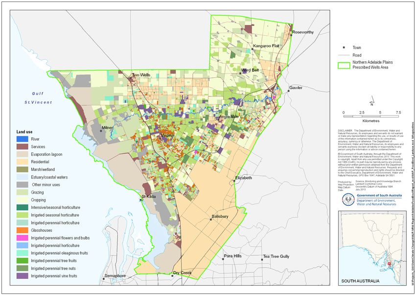
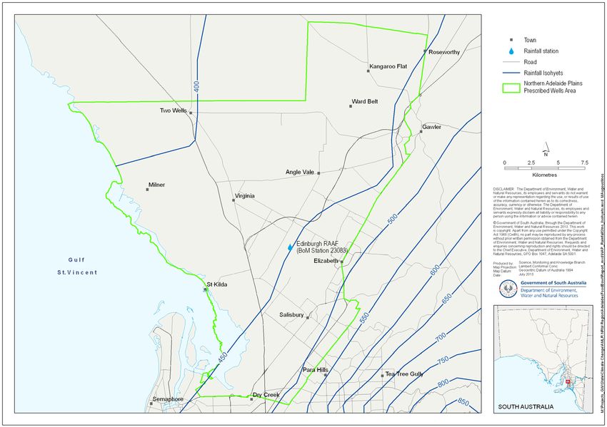
1. INTRODUCTION
The Adelaide and Mount Lofty Ranges (AMLR) Natural Resources Management (NRM) Region is working with key stakeholders
to help the NRM sector understand the likely impacts of climate change in the AMLR Region and promote the integration of
climate change into short and long-term risk management for sustainable NRM (AMLRNRMB, 2007).

This report is a product of the AMLRNRM Region project Building Capacity in Adelaide’s Food Bowl, which aims to build
knowledge and adaptation capacity amongst horticulturalists in the Northern Adelaide Plains (NAP) in order that horticultural
businesses are well prepared to adapt to the impacts of climate change.

The aim of this study is to evaluate the potential impacts of climate change and limited water availability on the irrigated
horticulture industry of the NAP. Projections of future climate from a suite of three Global Climate Models (GCMs) have been
downscaled from regional-scale model outputs to the local scale of the NAP. The downscaled projections of future climate
have been used to identify potential changes in daily temperature and rainfall patterns, and also changes in ‘weather event
indicators’, against which climate-related risks to horticultural crops in the region can be identified.

This study is focussed on indicators of climate change that may affect field-irrigated horticultural crops, and has been limited
to those crops that currently occupy the greatest area of irrigated land, namely potatoes, olives, wine grapes, almonds, carrots
and lettuce. Other primary industry sectors (e.g. protected horticulture, field crops, livestock etc.) are beyond the scope of this
investigation.

This report draws on findings of the Department of Environment, Water and Natural Resources (DEWNR) project Impacts of
Climate Change on Water Resources, Adelaide and Mount Lofty Ranges Natural Resources Management Region (Alcoe et al., in
prep.), in which numerical groundwater models were used to evaluate the potential impacts to groundwater availability under a
range of potential future climate scenarios. The climate projection selection and downscaling methods applied in DEWNR’s
regional Impacts of Climate change on Water Resources projects have also been adopted for use in this study.

The main findings of this study include the need to identify new sources of water as the principal strategy to assist growers
adapt to a future changing climate. It is also likely that alternative growing systems may need to be considered and new
cultivars be explored to aid in the mitigation of the potential impacts of climate change, such as warmer winters and increasing
heat, drought, disease and soil salinity.

1.1. The Adelaide Plains
The Adelaide Plains lie between the Western Mount Lofty Ranges and Gulf St Vincent. The main land uses are (1) urban
development to the south; (2) horticulture and viticulture across the central extent (i.e. the NAP); and (3) cereal grain cropping
and sheep grazing toward the north (Fig. 2). Water resources in the Northern Adelaide Plains (NAP) Prescribed Wells Area
(PWA) (Fig. 3) are managed through the NAP PWA water allocation plan. A new water allocation plan for the Adelaide Plains is
currently in preparation and will review and incorporate the existing Northern Adelaide Plains water allocation plan, as well as
including the Central Adelaide and Dry Creek prescribed wells areas for the first time.

The NAP horticultural district has been a significant producer of high-value horticultural crops since the late 1950’s with much
of its success attributed to its proximity to the city of Adelaide. The NAP also has high quality, well-drained sandy soils and
access to reliable water sources for irrigation. High quality underground water from confined sand and limestone aquifers
beneath the plains has supplied NAP irrigators for many years and since 1999 this has been supplemented by tertiary-treated
wastewater delivered via a pipeline network from the Bolivar wastewater treatment plant.

These features make the NAP conducive to the production, and efficient distribution, of a wide range of annual market garden
crops and perennial tree and vine fruit. However, horticulture in the NAP is vulnerable to the potential impacts of climate
change and there is a need for producers to understand the potential implications of climate change for their current and
planned cropping systems to assist in making informed investment decisions.

1.2. Climate of the Adelaide Plains
The Adelaide Plains has a Mediterranean-type climate with hot, dry summers and mild, wet winters. The majority of Adelaide’s
precipitation falls between the months of April to October, although rainfall exceeds potential evapotranspiration only in June

DEWNR Technical note 2013/09 3

and July (Fig 1). Contrastingly, in the Western Mount Lofty Ranges (e.g. Uraidla), rainfall exceeds potential evapotranspiration
between April and September. This water deficit is discussed in more detail in Section 3.4.

The marked elevation gradient of the western front of the Mount Lofty Ranges results in a rainfall gradient that follows the
prevailing direction of rainfall— i.e. west to east across the plains—from around 400 mm/y near the coast to around 650 mm/y
at the foot of the ranges (Fig. 3).

 200

 150
 Monthly average rainfall/PET (mm)

 100 Uraidla rainfall
 Edinburgh rainfall
 Uraidla PET
 Edinburgh PET

 50

 0

Figure 1. Average monthly rainfall and potential evapotranspiration for Edinburgh (BoM Station 23083) in
the Northern Adelaide Plains for the period 1889–2013, and for Uraidla (BoM Station 23750) in the
Western Mount Lofty Ranges for the period 1913–2012. Data source: SILO Climate Data (DSITIA, 2013)

DEWNR Technical note 2013/09 4

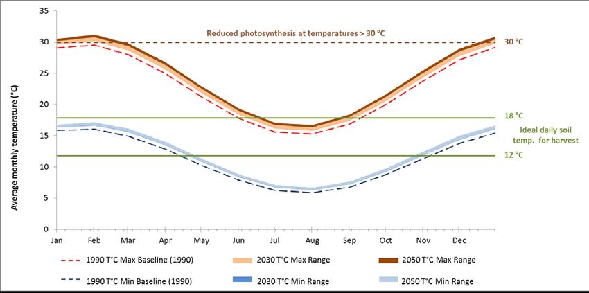
Figure 2. Land use

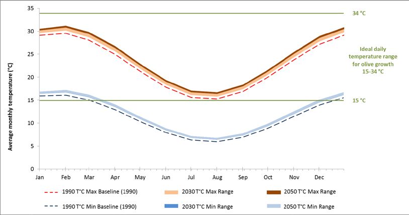
Figure 3. Location map showing rainfall isohyets

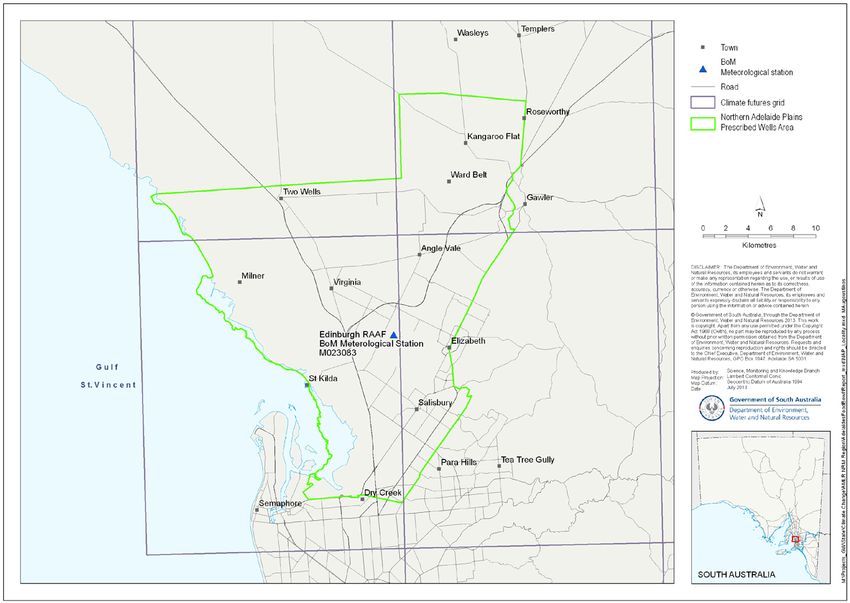
2. METHODS
Global Climate Models (GCMs) are mathematical representations of the physical processes that link together the atmosphere,
oceans, land surface and the sun. The output from GCMs differ from weather forecasts in that weather forecasts aim to predict
local-scale weather patterns over the time span of a few days, whereas GCMs are used to make regional-scale projections of
the trends in climate over time spans of years or decades. In this study, projections of future climate using GCMs requires the
regional-scale outputs of GCMs (where the dimensions of output grid cells are typically in the order of hundreds kilometres) to
be scaled down such that the data can be used in local-scale models (these require input grid cell sizes typically in the order of
a few kilometres).

There is a variety of GCMs that have been developed by various climate research organisations, from which one could select
models for use in climate change studies. Rather than applying a large number of GCMs, one approach is to use a small
number of GCMs can be selected that 1) represent most of the range of change projected by models and 2) have
demonstrated suitable accuracy on the historical climate for the particular geographical location, hence assuming that the
projections of future climate will also be representative . There are a number of approaches available to assist in their selection.
In this study, the Climate Futures Framework was applied, an approach developed by the Commonwealth Science and Industry
Research Organisation (CSIRO). (see section 2.2 and Appendix B)

It is important to note the difference between the terms ‘prediction’ and ‘projection’ in climate modelling. A prediction is a
forecast of future events based purely on historical observations. For example, a prediction could be based on a simple
extrapolation of historical trends. Daily weather forecasts would be considered predictions, because the forecast is based on
current atmospheric conditions, and those of the recent past. A projection, however, is an extrapolation of historical trends that
is dependent on certain assumptions holding true in the future. In the case of climate science, projections of future climate are
made that are dependent, for example, on a particular greenhouse gas emissions scenario playing out in the future.

Because nobody can be certain of which greenhouse gas emissions pathway will play out in the future, climate scientists report
climate projections based on a number of possible scenarios of future greenhouse gas emissions and resulting atmospheric
concentrations. By considering a number of GCMs and a number of emissions scenarios, a range of climate projections are
generated, and these are a reflection of the uncertainty in both the output of the models and in the emissions pathways that
might eventuate in the future. In this study, climate projections have been based on three GCMs and two greenhouse gas
emissions scenarios (high and low emissions), and the results have been projected out to two future time horizons (2030 and
2050).

This section briefly describes the methods used to generate the climate data used in this study. An expanded discussion
explaining these methods is included as appendices at the end of this report, whilst a more-detailed technical description of
the methodologies is presented in DEWNR Technical Reports, and these reports are indicated in the discussion that follows.

2.1. Climate data downscaling
Global Climate Models (GCMs) are the best tools available for simulating global and regional climate systems, and simulating
the changes that may occur due to increases in greenhouse gas concentrations. Generally, these models provide reasonable
representations of past trends over large spatial scales for a number of climate variables, such as temperature and air pressure.
However, GCM results are too coarse to be adopted directly in local-scale models and consequently, ‘downscaling’ of the
projections to the local weather-station scale is required. A brief summary of the downscaling techniques used to generate the
climate data used in this study is presented in Appendix A, and a complete description of the methodology can be found in
Gibbs et al. (2011). The downscaled data used in this study are at the daily time scale.

2.2. Global climate model selection: Climate Futures Framework
The Climate Futures Framework approach involves classifying the projected changes in climate by a range of GCMs into three
separate categories (termed Climate Futures) defined by two climate variables – here, the change in annual mean surface
temperature and the change in annual average rainfall have been used. Each Climate Future is then assigned a relative
likelihood, based on the number of climate models that fall within that category (Clarke et al., 2011). The different Climate
Future categories — defined as, for example ‘warmer, drier’, ‘warmer, slightly drier’ or ‘slightly warmer, slightly drier’ category
GCMs — can then be used as the basis for further impact assessment. A brief summary of the Climate Futures Framework used

DEWNR Technical note 2013/09 7

to select appropriate GCMs for use in this study is presented in Appendix B, and a complete description of the methodology
can be found in Alcoe et al. (in prep.).

2.3. Potential evapotranspiration
The potential evapotranspiration (PET) of a region is a variable of critical importance to horticulturalists as it directly affects the
water requirements of a certain crop type or land use within that region. Of the selected GCMs used in this study, none
produce projections of PET, necessitating estimation of PET from the projected data available, namely temperature and
humidity. There are many approaches to estimating PET from climate data and, in this study, one approach was selected from a
suite of five possible options (Appendix C). The approach used to estimate PET (Option 4) uses maximum temperature and the
relative humidity at that temperature. A complete description of the methodology used to estimate PET can be found in
Appendix C.

2.4. Dormancy breaking periods of ‘chilling’
Many perennial crops require a period of ‘chilling’, through the dormancy period, to trigger flower bud development and a
synchronised bud break. For the purpose of this study, the accumulation of chilling hours was assessed between the months of
May and September. Two commonly used chilling models were evaluated:

• The accumulation of hours at temperatures

3. CLIMATE CHANGE PROJECTIONS FOR THE NORTHERN
ADELAIDE PLAINS
The downscaled climate data for future climate scenarios for all three GCMs has been summarised (Tables 2–4) and a number
of ‘weather event indicators’ have been reported. The implications of these changes for horticulture are examined later in this
report, where potential climate change impacts to the main crop types are discussed individually and in more detail (Sect. 4).

Each of the tables presented in this section (Tables 2–4) summarises projected climate data for a single GCM – i.e. one table
each for (1) the ‘most-likely case’ or ‘warmer and slightly drier’ (MIROC-H GCM, (2) the ‘worst-case’ or ‘warmer and drier’
(CSIRO mk 3.5 GCM), and (3) the ‘best-case’, ‘slightly warmer, slightly drier’ (BCCR GCM) (Appendix B). Although selected as
the ‘most-likely’ GCM, the MIROC-H does project relatively large increases in temperature and thus the results presented
herein give reference to all three GCM outputs, resulting in a comprehensive range of potential future outcomes.

3.1. High-rainfall and low-rainfall years
Analyses of changes to average annual rainfall over the 30-year simulation period include projected percentage changes in the
number of high and low-rainfall years, characterised by the 80th percentile and 20th percentile average annual rainfall,
respectively. By definition, the 80th percentile is the value of annual rainfall totals below which 80% of annual rainfall totals lie.
Any year in which the average annual rainfall is projected to be greater than the 80th percentile has been defined to be a high-
rainfall year. The same rationale has been applied to the 20th percentile low-rainfall years. Hence, the historic baseline (1990)
low (20th percentile) and high (80th percentile) annual average rainfall amounts are respectively 363.4 mm/y and 473.9 mm/y
(Tables 2–4). As an example of relative change in high and low-rainfall years, for models run with the ‘most-likely case (MIROC-
H GCM), and for climate projections for the 2050 A2 scenario (Table 2), the 20th and 80th percentile rainfall amounts are
reduced to 354.1 mm and 471.6 mm, respectively. The percentage of years that would have historically been considered low-
rainfall years (less than 1990 20th percentile rainfall) increases from 20% to 29% in a 30-year sequence. The number of years
that would have historically been considered high-rainfall years (greater than 1990 80th percentile rainfall) reduces from 20% to
17% in a 30-year sequence.

3.2. Weather-event indicators
The ‘weather-event indicators’ are intended to give an insight into how some of the extremes in climate variables may change
in the future. The indicators have been based on generalised climatic vulnerabilities of the main unprotected crop types grown
across the NAP.

3.2.1. Heatwave
Protracted periods of extreme heat represent a high risk to growers due to potential loss of crop quality and yield as a result of
heat damage. Although different crop types have different sensitivities to heat changes with stage of crop development—and
indeed different cultivars within a crop type may exhibit variable heat tolerances—a conventional definition of heatwave has
been adopted in this study to enable a comparison of the annual occurrence of heatwave events between the 30-year baseline
(1990) climate and the climate projections for the future.

There is no universal definition of a heatwave. For the purposes of this study, a heatwave has been defined as a period of at
least 5 consecutive days where, on each of those days, the daily maximum temperature exceeds 35 °C. The annual occurrence
of heatwaves has then been reported as the number of heatwaves per year. For many biological systems, it is the combination
of hot days and hot nights that is important. Consequently, a similar approach has been taken with definition of a heatwave of
high overnight minimum temperatures, which is based on the annual occurrence of at least 5 consecutive nights where the
overnight minimum temperature exceeds 20 °C. These spells of relatively-high overnight minima have also been reported as
the number of occurrences per year.

3.2.2. Frost
An index of the risk to crops from frost has been defined as the number of days per year, between May and October, where the
daily minimum temperature in the Stevenson screen is less than 1 °C (the temperature nominated by the Bureau of

DEWNR Technical note 2013/09 9

Meteorology as an indicator of frost risk). Also, the maximum frost-free period (number of consecutive days where the daily
minimum temperature is greater than, or equal to, 1 °C) has been calculated. For each of these indices, the percentage change
for each scenario from the 1990 baseline period has been reported.

3.2.3. Rainfall at harvest
An index of the risk to crops from ‘rainfall at harvest’ has been defined as the number of rainfall events that occur between
February and April, and in which rainfall is greater than 4 mm/day. The percentage change for each scenario from the 1990
baseline period has also been reported. It should be noted that the downscaling approach adopted scales the observed rainfall
by different amounts depending on the original rainfall amount and the season. As such, there is no change to the days when
rainfall does or does not occur. A more sophisticated approach is required to represent these changes, for example that being
developed by the Goyder Institute Project Developing an Agreed Set of Climate Change Data for South Australia.

3.3.TIME PERIODS FOR PROJECTIONS OF BASELINE AND FUTURE CLIMATES
Future climate datasets have been projected at the time horizons of 2030 and 2050 and for low and high-emissions scenarios.
Climate statistics have been reported as ‘average annual’ data that have been calculated over a 30-year period. These 30-year
periods are centred around the future time horizons of 2030 and 2050. Also reported is the percentage change in climate data
between (1) the future time horizons and (2) a 1990 baseline period. The 1990 baseline period is a 30-year climate dataset
(1975–2004) comprising historical, measured climate data that has been recorded at the Edinburgh weather station (BoM
Station 023083). The projected 2030 and 2050 future climate datasets were downscaled from regional-scale GCM outputs to
the Edinburgh weather station locale (Sect. 2.1; Appendix A).

The summary climate data in the following tables have been calculated from GCM projections of daily temperature and daily
rainfall.

DEWNR Technical note 2013/09 10

Table 2. Changes in climate and ‘weather-event indicators’ simulated for the Northern Adelaide Plains
using input data generated using the MIROC-H GCM (warmer, slightly drier category GCM)

 MIROC-H (‘most-likely’ case) GCM
 Edinburgh, SA (BOM station 023083) 1990 # 2030# 2050#
 B1 A2 B1 A2

 AVERAGE ANNUAL CLIMATE DATA
 Rainfall (mm) 423.5 412.6 406.7 412.4 402.1
 Change from 1990 baseline (%) -3 -4 -3 -5
 th
 20 percentile (mm) 363.4 355.2 352.2 354.1 349.6
 % of years < 1990 20th percentile 20 23 27 25 30
 th
 80 percentile (mm) 473.9 468.7 461.4 471.6 459.5
 th
 % of years > 1990 80 percentile 20 19 17 19 17
 Potential Evapotranspiration (mm) 1311.3 1352.5 1373.9 1355.2 1391.7
 Change from 1990 baseline (%) 3 5 3 6
 Maximum Temperature (TMax °C) 22.4 23.1 23.4 23.1 23.7
 Change from 1990 baseline (°C) 0.7 1.0 0.7 1.3
 Minimum Temperature (TMin °C) 11.0 11.5 11.8 11.6 12.0
 Change from 1990 baseline (°C) 0.5 0.8 0.6 1.0
 Average Temperature (TAve °C) 16.7 17.3 17.6 17.4 17.9
 Change from 1990 baseline (°C) 0.6 0.9 0.7 1.2
 HEATWAVE (Oct – Apr)
 Number of days where TMax > 35 °C 23.7 28.0 30.4 28.5 32.8
 Change from 1990 baseline (%) 18 28 20 38
 Annual occurrences of 5 consecutive
 0.9 1.1 1.3 1.1 1.4
 days where TMax > 35 °C
 Change from 1990 baseline (%) 19 48 26 56
 Number of days where TMin > 20 °C 20.5 24.3 28.1 24.7 30.3
 Change from 1990 baseline (%) 18 37 20 48
 Annual occurrences of 5 consecutive
 0.8 1.0 1.2 1.0 1.6
 nights where TMin > 20 °C
 Change from 1990 baseline (%) 30 61 35 109

 FROST (May – Oct)
 Number of days where TMin < 1 °C 3.8 2.8 2.8 2.8 2.7
 Change from 1990 baseline (%) -27 -27 -27 -30
 Frost free period (days) 297.8 297.8 298.5 297.8 298.5
 Change from 1990 baseline (%) 0.0 0.2 0.0 0.2
 RAIN AT HARVEST (Feb - Apr)
 Rain events >4 mm/day 4.4 4.3 4.3 4.1 3.4
 Change from 1990 baseline (%) -4 -4 -8 -23
 # Amounts stated are annual averages or occurrences in a projected or historic 30-year time period (Sect. 3.3)

DEWNR Technical note 2013/09 11

Table 3. Changes in climate and weather event indicators simulated for the Northern Adelaide Plains
using input data generated using the BCCR GCM (slightly warmer, slightly drier category GCM)

 BCCR (‘best’ case) GCM
 Edinburgh, SA (BOM station 023083) 1990 # 2030# 2050#
 B1 A2 B1 A2

 AVERAGE ANNUAL CLIMATE DATA
 Rainfall (mm) 423.5 404.6 395.0 403.2 387.9
 Change from 1990 baseline (%) -5 -7 -5 -8
 th
 20 percentile (mm) 363.4 341.2 333.2 341.6 328.7
 th
 % of years < 1990 20 percentile 20 28 32 29 36
 80th percentile (mm) 473.9 457.4 446.8 458.9 441.1
 th
 % of years > 1990 80 percentile 20 16 11 17 10
 Potential Evapotranspiration (mm) 1311.3 1346.2 1364.6 1348.7 1379.2
 Change from 1990 baseline (%) 3 4 3 5
 Maximum Temperature (TMax °C) 22.4 23.0 23.3 23.1 23.6
 Change from 1990 baseline (°C) 0.6 0.9 0.7 1.2
 Minimum Temperature (TMin °C) 11.0 11.6 11.9 11.6 12.1
 Change from 1990 baseline (°C) 0.6 0.9 0.6 1.1
 Average Temperature (TAve °C) 16.7 17.3 17.6 17.3 17.8
 Change from 1990 baseline (°C) 0.6 0.9 0.6 1.1
 HEATWAVE (Oct – Apr)
 Number of days where TMax > 35°C 23.7 27.2 29.9 27.5 31.2
 Change from 1990 baseline (%) 15 26 16 32
 Annual occurrences of 5 consecutive
 0.9 1.0 1.3 1.0 1.4
 days where TMax > 35 °C
 Change from 1990 baseline (%) 15 44 15 52
 Number of nights where TMin > 20 °C 20.5 25.0 28.5 25.2 31.0
 Change from 1990 baseline (%) 22 39 23 51
 Annual occurrences of 5 consecutive
 0.8 1.1 1.3 1.1 1.7
 nights where TMin > 20 °C
 Change from 1990 baseline (%) 39 65 39 122

 FROST (May – Oct)
 Number of days where TMin < 1 °C 3.8 2.8 2.8 2.8 2.7
 Change from 1990 baseline (%) -27 -27 -27 -30
 Frost free period (days) 297.8 297.8 298.5 297.8 298.5
 Change from 1990 baseline (%) 0.0 0.2 0.0 0.2
 RAIN AT HARVEST (Feb - Apr)
 Rain events >4 mm/day 4.4 4.1 4.1 4.7 4.7
 Change from 1990 baseline (%) -8 -8 6 7
 # Amounts stated are annual averages or occurrences in a projected or historic 30-year time period (Sect. 3.3)

DEWNR Technical note 2013/09 12

Table 4. Changes in climate and weather event indicators simulated for the Northern Adelaide Plains
using input data generated using the CSIRO Mk3.5 GCM (warmer, drier category GCM)

 CSIRO Mk3.5 (‘worst’ case) GCM
 Edinburgh, SA (BOM station 023083) 1990 # 2030# 2050#
 B1 A2 B1 A2

 AVERAGE ANNUAL CLIMATE DATA
 Rainfall (mm) 423.5 375.7 352.8 372.0 336.4
 Change from 1990 baseline (%) -11 -17 -12 -21
 th
 20 percentile (mm) 363.4 316.0 297.4 313.4 279.4
 % of years < 1990 20th percentile 20 40 53 41 65
 th
 80 percentile (mm) 473.9 432.1 405.5 425.5 385.1
 th
 % of years > 1990 80 percentile 20 9 5 7 4
 Potential Evapotranspiration (mm) 1311.3 1358.0 1382.9 1361.3 1402.4
 Change from 1990 baseline (%) 4 6 4 7
 Maximum Temperature (TMax °C) 22.4 23.2 23.7 23.3 24.0
 Change from 1990 baseline (°C) 0.8 1.3 0.9 1.6
 Minimum Temperature (TMin °C) 11.0 11.7 12.0 11.7 12.3
 Change from 1990 baseline (°C) 0.7 1.0 0.7 1.3
 Average Temperature (TAve °C) 16.7 17.5 17.8 17.5 18.2
 Change from 1990 baseline (°C) 0.8 1.1 0.8 1.5
 HEATWAVE (Oct – Apr)
 Number of days where TMax > 35 °C 23.7 28.7 31.9 29.6 34.8
 Change from 1990 baseline (%) 21 35 25 47
 Annual occurrences of 5 consecutive
 0.9 1.1 1.4 1.3 1.7
 days where TMax > 35 °C
 Change from 1990 baseline (%) 26 52 44 89
 Number of days where TMin > 20 °C 20.5 26.1 30.0 26.4 32.7
 Change from 1990 baseline (%) 27 47 29 60
 Annual occurrences of 5 consecutive
 0.8 1.1 1.6 1.2 1.8
 nights where TMin > 20 °C
 Change from 1990 baseline (%) 48 109 57 135

 FROST (May – Oct)
 Number of days where TMin < 1 °C 3.8 2.8 2.7 2.8 2.7
 Change from 1990 baseline (%) -27 -30 -27 -30
 Frost free period (days) 297.8 297.8 298.5 297.8 298.5
 Change from 1990 baseline (%) 0.0 0.2 0.0 0.2
 RAIN AT HARVEST (Feb - Apr)
 Rain events >4 mm/day 4.4 4.0 3.7 3.6 4.1
 Change from 1990 baseline (%) -9 -17 -18 -8
 # Amounts stated are annual averages or occurrences in a projected or historic 30-year time period (Sect. 3.3)

DEWNR Technical note 2013/09 13

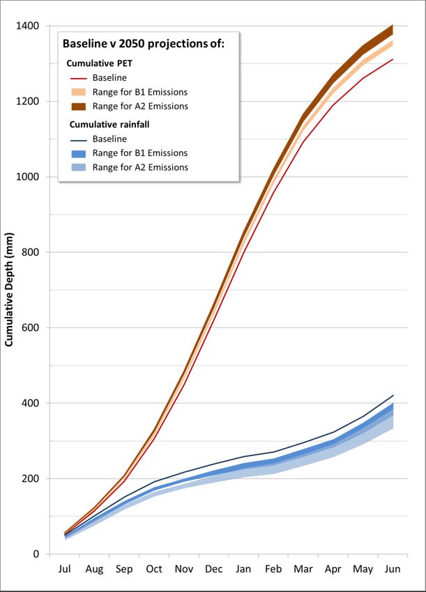
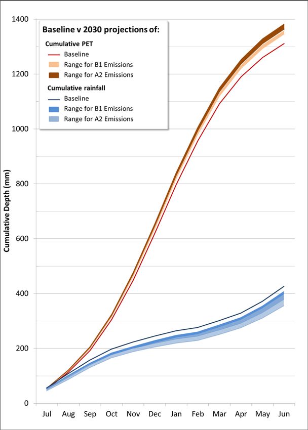
3.4. Rainfall, potential evapotranspiration and irrigation water deficit
Optimum crop growth can only occur when water is not limiting. The concept of ‘water deficit’ is commonly defined as a shortage of available water through the deficit between the rate of
incident rainfall and the rate of potential evapotranspiration. The cumulative water deficit over the course of the water-use year may give an indication of the amount of irrigation that would be
required to meet the water deficit. A range of water deficits has been estimated for the average water-use year for the range of projected climates at 2030 and at 2050 and also for the 1990
baseline period (Fig. 4). The range of projected water deficits is a reflection of the uncertainties in different GCMs and also the emissions scenario pathways that might play out in the future, as
discussed at the beginning of Section 2.

Figure 4. Comparison of cumulative baseline (1990) rain and PET with the range of 2030 and 2050 GCM projections for B1 and A2 emission scenarios.

Water deficits have also been presented as average monthly totals (Fig. 5), for the 12 projected future climate scenarios and also for the 1990 baseline period, and are shown only for the
irrigation period of September–April. An estimate of the total irrigation water required for the year is presented on the far right of each chart (note the two different scales on each of the two
vertical axes).

.
Figure 5. Monthly average water deficits (PET minus Rainfall) plus total water deficit through the irrigation season (Sep–Apr) for the BCCR, MIROC-H and
CSIRO Mk 3.5 GCMs relative to the 1990-baseline period

3.5. CHILLING
Many perennial crops require a period of ‘chilling’, during dormancy, to trigger flower bud development and a synchronised
bud break. While chilling requirements are both crop and variety-specific, the response to insufficient chill is consistent across
most crops and includes a reduced and protracted bud break which in turn can bring about a cycle of biennial bearing. The
projected change in chilling has been evaluated using two different chill accumulation models (Figs 6 and 7). Both models
make use of disaggregated hourly observations of daily temperature between May and September. ‘Chill hours’ are the
accumulation of hours where the observed temperature is less than 7.2 °C (Sect. 2.4.). ‘Richardson Chill Units’ are calculated
using a more-complex model, designed to account for the relative contribution of different temperatures on chill accumulation
(Sect. 2.4.). While each model accounts for the impact of warming differently, both reflect a reducing trend in chill
accumulation, when comparing the 12 future scenarios against the 1990 baseline period.

Figure 6. Projected change in dormancy breaking ‘chill hours’ (Sect. 2.4). Comparison of baseline (1990)
scenario to those of BCCR, MIROC-H and CSIRO Mk 3.5 GCMs at two time horizons and two emission
scenarios.

Figure 7. Projected change in dormancy breaking ‘Richardson chill units’ (Sect. 2.4). Comparison of
baseline (1990) scenario to those of the BCCR, MIROC-H and CSIRO Mk 3.5 GCMs at two time horizons and
two emission scenarios.

DEWNR Technical note 2013/09 16

4. CROP RESPONSE TO PROJECTED CLIMATE CHANGE SCENARIOS
The results tables presented in this section (Tables 5–10) are intended to indicate potential implications of the direction of
change in the projected future climate of the NAP over the longer term (e.g. increasing heatwave frequency in the future as a
result of climate change, and what is the likely impact of this change on a particular crop type). In view of this, the results
reported here are based on the MIROC-H GCM under the high-emissions scenario at the more-distant time horizon of 2050.
The MIROC-H GCM was selected here as it satisfies the requirements outlined by Clarke et al. (2011) necessary for classification
as a ‘most likely’ case GCM (refer Appendix B). An indication of the short-term impacts (i.e. 2030) — or impacts according to
the alternative (BCCR, CSIRO Mk3.5) GCMs — can be deduced by reading off projections of climate change from the different
GCMs, emissions scenarios and time horizons listed in Tables 2–4 and substituting these data into Tables 5–10.

DEWNR Technical note 2013/09 17

4.1. Potatoes
The South Australian potato industry occupies approximately 11 900 ha and produces an average annual crop of over 300 000
tonnes (ABS, 2007). The NAP potato growing region is an important part of the SA industry supplying 14% of the state’s
production. Almost all the NAP crop is marketed as fresh product, making quality as important an issue as yield for local
growers. Both yield and quality are closely linked to the prevailing climate.

Temperature influences potato yields both directly, through daily effects on growth rates, and indirectly, through seasonal
effects on the length of the crops growth cycle (Kooman, 1994) (Fig. 8). While potatoes are known for their adaptability to a
wide range of growing temperatures, particularly during periods of longer day length, their growth slows significantly when the
daily average temperature is below 5 °C or above 21 °C (Haverkort & Verhagen, 2008) and their photosynthetic capacity halts
completely at temperatures below 2 °C and above 35 °C (Fig. 9). In order to continue cropping in spring and autumn,
producers will likely need to source cultivars with growth cycles suited to shorter and warmer winter and longer and hotter
summer periods. It is likely that cultivar selection criteria for NAP potato producers will need to include tolerance to reduced
water availability and temperature extremes, particularly heat.

 35

 30

 25
 Average monthly temperature (°C)

 21 °C
 20

 15

 10
 Period of 'ideal' average temperature projected to
 decrease by 13-35 days.
 5 5 °C

 0
 Jan Feb Mar Apr May Jun Jul Aug Sep Oct Nov Dec

 1990 T°C Avg Baseline (1990) 2030 T°C Avg Range 2050 T°C Avg Range

Figure 8. Effect of projected increase in average monthly TAvg on ‘optimum’ potato growing conditions

Figure 9. Average monthly TMax and TMin projections for baseline (1990), 2030 and 2050 climate scenarios
with daily thresholds for potato photosynthetic capacity and pre-harvest soil temperature

DEWNR Technical note 2013/09 18

Table 5. Significance of MIROC-H (‘most-likely’ case) climate projection for NAP Potato production.
 Climate 1990 v 20504 Significance for Potato production
 parameter Change projected by MIROC-H
 GCM with A2 emission scenario 
 Mean TAvg projected to increase by 7% Length of growth cycle likely to be compressed with potential
 temperature (1990 = 16.7 °C, 2050 = 17.9 °C) negative implications on tuber size (Franke et al., 2013).
 Higher temperatures assumed to favour foliar rather than tuber
 growth.
 Optimum growth period, where TAvg = 5-21 °C, projected to
 decrease by up to 35 days by 2050 (Fig. 8).
 Current climate allows for spring and autumn cropping
 (PotatoesSA, 2013). Projected change is likely to favour the
 autumn cropping period (winter harvest).
 Greater care may be required when targeting spring crops
 (summer harvest). For example, there may be an increased
 dependence on pre-harvest irrigation events to bring soil
 temperature close to ideal harvest temperature of 12–18 °C.
 Harvesting outside this range increases bruising and
 microbiological decays (Johnstone, 2012).
 The potential shift to warmer growing seasons may increase pest
 and disease pressure as higher temperatures allow more cycles of
 pathogen multiplication (Haverkort & Verhagen, 2008).
 Extreme heat Extreme heat days projected to Photosynthetic capacity reduces when temperatures exceed 30 °C
 days 1 increase by 38% and ceases completely when greater than 35 °C (Franke et al.,
 & (1990 = 24 days/y, 2050 = 33 2013).
 Heatwaves 2 days/y) Extended periods of high temperatures may increase leaf
 Heatwaves projected to increase by senescence with deleterious implications for photosynthesis and
 56% yield.
 (1990=0.9 events/y, 2050=1.4 Tuber initiation may be inhibited at higher temperatures.
 events/y) Increased soil moisture deficits and elevated soil temperatures
 may be experienced. Both may be exacerbated by reduced leaf
 cover.
 Frost 3 Frost events projected to reduce by Reduced risk of frost is favourable for this frost sensitive crop.
 30% Some potato cultivars present symptoms at temperatures as high
 (1990 = 3.8 days/y, 2050 = 2.8 as 3 °C (Wale et al., 2008).
 days/y) Plants can recover from exposure to frost, but successive frost
 events will have negative implications for sizing and quality.
 Despite a reduced incidence of frost on the NAP, the likelihood of
 compressed phenology may mean that frost sensitive growth
 stages remain at risk.
 Mean rainfall Rainfall projected to reduce by 5% While potatoes are intolerant to waterlogging, they do require a
 & (1990 = 424 mm/y, 2050 = 402 steady supply of water throughout the growing season.
 PET mm/y) Low soil moisture during tuber initiation results in fewer tubers.
 Low soil moisture during the bulking phase results in small,
 PET projected to increase by 6% misshapen tubers.
 (1990 =1311 mm/y, 2050 =1392 Low moisture availability also increases the potential for poor
 mm/y) quality through secondary growths, scab and hollow heart.
 Producers will likely need to source additional volumes of
 irrigation water to satisfy plant water requirements.
 Soil salinity may become more prominent if increased volumes of
 low quality water are applied. This may be exacerbated if there is
 reduced occurrence of winter leaching rain.
 Refer to Table 2 for more complete description of change projected by the MIROC-H GCM
1 Extreme heat days = days where TMax >35 °C
2 Heatwave = five consecutive extreme heat days

3 Frost events = days where T
 Min

4.2. Olives
South Australia’s prevailing climate has long been seen as ideal for olive production, particularly given its similarity to that of
the Mediterranean Basin where most of the world’s olives are grown (Sweeney, 2006). Over 900 ha of the NAP is currently
planted to olives, which accounts for more than 20% of the state’s planting (ABS, 2007), and is largely operated under small to
medium sized holdings of fewer than 10 000 trees. Almost all olives from the NAP region are destined for oil production.

The ideal daily temperature range for olive growth is between 15–34 °C, with performance declining when daily maximum
exceeds 40 °C or the daily minimum drops below 5 °C (Taylor & Burt, 2007). Given the tolerance of the olive plant to heat, and
its preference for a long hot growing season, the NAP olive industry is likely to remain viable despite the projected increases in
temperature (Fig. 10). However, increasing temperatures imply reduced chilling through the dormancy period (Figs 6 & 7).
Most olive varieties have low chilling requirements, with average July temperatures below 10-12 °C often being adequate
(Kailis & Harris, 2007). Baseline conditions show that the NAP only narrowly meets the chilling requirement for most olive
varieties and a warming climate will put further pressure on this chill period (Fig. 11). Furthermore, projections from the
MIROC-H GCM under a high-emissions scenario suggest that the frequency of days where the maximum temperatures exceed
40 °C is projected to almost double, from 4.8 days/y in the 1990 baseline period to 9.4 days/y by 2050. Maintaining plant water
status through these extreme heat events will be important in producing commercial parcels of fruit.

Figure 10. Average monthly TMax and TMin projections for baseline (1990), 2030 and 2050 climate scenarios
with daily temperature thresholds for olive growth. Refer to Table 6 for frequency of daily heat events.
 35

 30

 25
 Average monthly temperature (°C)

 20

 15
 Olives require July
 TAvg < 12 °C for
 10 successful flowering

 5 Dormancy breaking 'chill' period
 projected to decrease by 20-45 days

 0
 Jan Feb Mar Apr May Jun Jul Aug Sep Oct Nov Dec

 1990 T°C Avg Baseline (1990) 2030 T°C Avg Range 2050 T°C Avg Range

Figure 11. Projected increase in TAvg is likely to compress the dormancy breaking chill period for olives.

DEWNR Technical note 2013/09 20

Table 6. Significance of MIROC-H (‘most-likely’ case) climate projection for NAP Olive production.

Climate 1990 v 20504 Significance for Olive production
parameter Change projected by MIROC-H
 GCM with A2 emission scenario 
Mean TAvg projected to increase by 7% Olives are well adapted to warmer climates, ideal temperature
Temperature (1990 = 16.7 °C, 2050 = 17.9 °C) range 15- 34 °C (Taylor and Burt, 2007).
 Temperatures cooler than 10 °C can impede pollination (Kailis and
 Harris, 2007) and so warmer spring temperatures are likely to
 improve fruit set.
 Potential for advanced and compressed phenology if climate
 warms. Compressed growing season may lead to early harvest.
Extreme heat Extreme heat days projected to While olives prefer long hot growing season, performance declines
days 1 increase by 38% at temperatures greater than 40 °C. Such conditions are projected
& (1990 = 24 days/y, 2050 = 33 to almost double in frequency by 2050 (1990 = 4.8 days/y >40 °C,
Heatwaves 2 days/y) 2050 = 9.4 days/y >40 °C)
 Heatwaves projected to increase by Despite increased frequency of extreme heat days, the tree’s
 56 % adaptability to warmer climates makes the olive one of the crops
 (1990=0.9 events/y, 2050=1.4 least susceptible to a projected warming climate.
 events/y) Increased water requirements.
Frost 3 Frost events projected to reduce by Olives can tolerate severe frosts through dormancy but are
 30% particularly sensitive to it during flowering.
 (1990 = 3.8 days/y, 2050 = 2.8 While the frequency of frost events is projected to decline in the
 days/y) future, the drying climate may increase frost severity.
 Advancing phenology may result in olives remaining susceptible to
 frost events, the result being reduced yields.
Chilling Dormancy breaking chill period Successful flowering and fruit set requires a period of chilling
 projected to decrease by between through dormancy. Average July temperatures below 10-12 °C is
 20 and 45 days (Fig 11) adequate for most varieties (Kailis and Harris, 2007).
 Insufficient chill results in uneven and delayed bud break.
 Particularly warm winters may see complete bud failure (i.e.
 increases in July Tavg imply an increase in the frequency of years
 where July Tavg is above 12°C).
Mean rainfall Rainfall projected to reduce by 5% Projected decreases in rainfall may result in reduced risk from some
& (1990 = 424 mm/y, 2050 = 402 diseases (e.g. phytophthora root rot, olive leaf spot and
PET mm/y) anthracnose fruit rot).
 There may be an increased risk of diseases that favour dry
 PET projected to increase by 6% conditions and water stressed plants (eg- charcoal root rot).
 Reduced rainfall through winter means less opportunity for pre-
 (1990 =1311 mm/y, 2050 =1392
 season filling of soil profile. Adequate soil moisture in spring is
 mm/y)
 essential for flower and fruit set.
 Extended periods of water stress could impact olive flowering,
 shoot growth and fruit quality.
 Producers will need to consider the availability of irrigation water
 to satisfy potentially increasing plant water requirements.
 Soil salinity may become more prominent if increased volumes of
 low quality irrigation water are applied. The issue may be
 exacerbated if there is a reduced occurrence of winter leaching rain
 events.
Rain near Rain near harvest to reduce by 23% While unseasonal or extreme rain events are difficult to predict,
harvest (1990 = 4.4 days, 2050 = 3.4 days) projections for reduced rainfall through autumn is a favourable
 trend for olive oil producers. Oil yields can be compromised by
 high rain in autumn (Taylor and Burt, 2007).
 Refer to Table 4 for more complete description of change projected by the MIROC-H GCM
1 Extreme heat days = days where TMax >35 °C
2 Heatwave = five consecutive extreme heat days

3 Frost events = days where T
 Min

4.3. Grapes
Wine grapes are planted to approximately 600 ha on the NAP. While representing only a small component of the state’s total
grape crush, the estimated value of the 2013 crush was significant for the region at greater than $3M (PGIBSA, 2013). In 2013,
the total intake of grapes from the NAP was over 3800 tonnes, 62% of which were red varietals comprising largely Shiraz
(PGIBSA, 2013).

One of the more significant implications of a changing climate for the wine industry is the potential for advanced vine
phenology. For recent Australian vintages, advanced phenology has equated to a rate of change in maturity of 9.3 ±2.67 days
per °C (Petrie & Sadras, 2008). For NAP vines, this could mean an advancement of up to 18 days by 2050, for the ‘worst-case’
GCM projection under a high-emissions scenario. The advanced maturity is largely driven by an earlier onset of berry ripening
(Sadras & Petrie, 2011) and means that the ripening process is likely to occur during warmer times of the year. Ripening under
warmer conditions influences acid levels, the accumulation of sugars as well as complicating the development of berry flavour
and colour. These changes imply impacts to the flavour balance and alcohol content of the wine. Advanced maturity also has
implications for harvest and winery operations, as production will be impacted by multiple parcels of fruit coming from large
plantings of overlapping varieties.

 Powdery mildew case study
 This case study has been included as an example of the type of projection and analysis possible when well
 defined climatic determinants are available for issues of relevance to crop performance.
 While wet weather is not required for the development of powdery mildew, its growth is hastened when
 relative humidity is >40 %. The ideal temperature range for powdery mildew growth is between 20 and 28 °C.
 While extreme heat days may slow growth, the cooler nights that follow these hot days are frequently within
 the ideal temperature range (Magarey, 2010). The result being that a warming climate may favour the
 development of powdery mildew and related diseases.
 The cumulative duration of hours where temperature and humidity met the ideal growing conditions for
 powdery mildew (THourly Avg 20 – 28 °C, RHDaily Avg >40 %) were compared between baseline and GCM scenarios.
 Hourly temperature data was disaggregated, from downscaled GCM data as per the method described by
 Linvill (1990).

 Table CS1. Average number of hours per day (Oct-Apr) where climatic conditions suit the
 growth of powdery mildew on grape vines. Projections of three GCM’s at two time horizons,
 2030 and 2050, and two emission scenarios, B1 and A2.

 Baseline 2030 2050
 GCM
 (1990) B1 A2 B1 A2
 BCCR (hours/day) 6.66 6.90 6.69 7.08
 Change from baseline (%) 8.1 12.0 8.5 14.8
 CSIRO Mk3.5 (hours/day) 6.78 7.06 6.81 7.31
 6.16
 Change from baseline (%) 10.1 14.6 10.5 18.6
 MIROC-H (hours/day) 6.63 6.84 6.66 7.01
 Change from baseline (%) 7.5 11.0 8.1 13.8

 Despite a drying climate, all GCM’s projected an increase in the conditions conducive to powdery mildew
 growth, moving from a baseline of 6.16 hours per day to between 6.63 and 7.31 hours per day per growing
 season, dependent on GCM scenario. This result highlights the importance of continued vigilance in the
 application of protective cover sprays from early in the season.

DEWNR Technical note 2013/09 22