Brief communication: How does complex terrain change the power curve of a wind turbine?
←
→
Page content transcription
If your browser does not render page correctly, please read the page content below
Wind Energ. Sci., 7, 1527–1532, 2022
https://doi.org/10.5194/wes-7-1527-2022
© Author(s) 2022. This work is distributed under
the Creative Commons Attribution 4.0 License.

               Brief communication: How does complex terrain
                  change the power curve of a wind turbine?
                 Niels Troldborg, Søren J. Andersen, Emily L. Hodgson, and Alexander Meyer Forsting
                      DTU Wind and Energy Systems, Frederiksborgvej 399, 4000, Roskilde, Denmark
                                       Correspondence: Niels Troldborg (niet@dtu.dk)

                                     Received: 14 March 2022 – Discussion started: 5 April 2022
                              Revised: 15 June 2022 – Accepted: 24 June 2022 – Published: 20 July 2022

       Abstract. The power performance of a wind turbine in complex terrain is studied by means of large eddy
       simulations (LESs). The simulations show that the turbine performance is significantly different compared to
       what should be expected from the available wind. The reason for this deviation is that the undisturbed flow field
       behind the turbine is non-homogeneous and therefore results in a very different wake development and induction
       than seen for a turbine in flat homogeneous terrain.

1   Introduction                                                    curve (Brodeur and Masson, 2008; Nam et al., 2004; Bor-
                                                                    raccino et al., 2017). However, to the best of our knowledge,
The power curve of a wind turbine shows the relationship            Oh and Kim (2015) are so far the only ones to investigate
between its power output and the undisturbed wind speed at          whether the power curve of a turbine is identical in flat and
hub height. In combination with estimates of the wind re-           complex terrain. They analysed the actual measured power
source, the power curve is used to predict the expected en-         curve of five wind turbines in a wind farm at a complex site
ergy yield of a wind turbine at a candidate site. Thus, the         and found large differences between the turbines as well as
power curve is one of the most important characteristics of a       with the power curve guaranteed by the manufacturer. They
wind turbine and therefore is also typically guaranteed by the      used the different power curves to predict the annual energy
manufacturer. Power performance verification tests are usu-         production (AEP) and found that the estimates based on the
ally conducted in flat homogeneous terrain where the undis-         measured curves could be up to 17.8 % lower than when us-
turbed wind speed is approximated by measuring sufficiently         ing the guaranteed power curve. A disadvantage of using
far upstream (typically 2.5 rotor diameters). In complex ter-       field measurements to analyse power performance in com-
rain this approach is invalid because the upstream flow in          plex terrain is that there inevitably will be uncertainties in the
this case is not homogeneous. Instead it is common practice         predicted power curve. The biggest uncertainty lies in deter-
to perform a site calibration prior to erecting the turbine in      mining the free-stream velocity, but a turbine may also per-
which the wind speed at the location of the turbine is related      form differently than expected due to, for example, erosion,
to the corresponding wind speed measured at some upstream           icing or blade surface contamination. In addition the stochas-
location.                                                           tic nature of the wind resource requires very long measure-
   An alternative to site calibration is to use a nacelle-          ment periods to obtain converged statistics.
mounted lidar to measure at several ranges closer to the rotor         Simulations on the other hand do not have these issues
and make proper corrections of the measured flow to account         and therefore are ideal for studying power curves and how
for the induction effect (Borraccino et al., 2017).                 they may change in complex terrain. Furthermore, it has been
   In either case the idea is to establish the free-stream con-     shown that simulations using both RANS (Allen et al., 2020;
ditions at the position of the turbine. Most work on wind tur-      Sessarego et al., 2018) and large eddy simulation (LES) (Liu
bine power performance verification in complex terrain fo-          et al., 2021; Yang et al., 2018; Shamsoddin and Porté-Agel,
cuses on how to establish a robust and accurate free-wind-
speed estimate and thereby reduce the scatter in the power

Published by Copernicus Publications on behalf of the European Academy of Wind Energy e.V.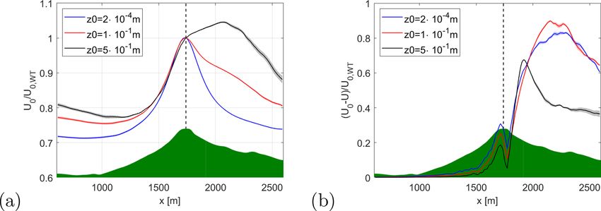
1528 N. Troldborg et al.: How does complex terrain change the power curve of a wind turbine?
2017) are reasonably accurate at predicting the power perfor- sub-grid stresses are modelled using the closure by Deardorff
mance of wind turbines in complex terrain. (1980).
However, the question as to how the terrain impacts the
power curve of a wind turbine still remains unanswered. The 3 Results
objective of the present work is to answer this question by
conducting LES of the power performance of a wind turbine In the following we present results from a series of simula-
in complex terrain and comparing this with the correspond- tions where u∗ is varied between 0.2 and 0.6 m s−1 and the
ing predictions in flat terrain. roughness height is varied between 2×10⁻⁴ and 0.5 m. More
details about the wind turbine inflow characteristics for each
case are provided in the Appendix. In each case we simulate
2 Methodology
1.5 h of real-time flow but only analyse the last hour in order
to get rid of any initial transients. Each 1 h simulation is split
In the following we consider a DTU 10 MW wind turbine
into 6 × 10 min sections from which we compute ensemble-
(Bak, 2013) operating in both flat and complex terrain. This
averaged 10 min statistics and evaluate the variability via the
turbine has a diameter of 178.34 m and a hub height of 119 m.
standard error of the mean.
The complex terrain is based on the topography at the site of
Figure 1 shows the power curve of the turbine in com-
Perdigão in Portugal consisting of two parallel ridges, and
plex and flat terrain as predicted by AD LES and standalone
the turbine is in this case placed on top of the first ridge.
Flex5, respectively (markers). The inflow for the standalone
The ratio between ridge height and turbine diameter is 1.5.
Flex5 simulations is extracted from the LES cases without
The curvilinear grid used to resolve the terrain is described
the turbine included. As reference (black lines), the power
in Berg et al. (2017) except that here it is extended with a
curves predicted by both methods at uniform laminar inflow
flat region after the terrain where the turbulence is allowed to
are also included. Note that the AD-LES reference curve is
dampen out before exiting the domain.
computed on a cubic grid as described by Hodgson et al.
The dimensions of both computational domains are Lx ×
(2021) but with a grid resolution which is similar to the one
Ly × Lz = 8480 m × 2560 m × 3081 m, where subscripts x,
used here for resolving the terrain.
y and z refer to the streamwise, spanwise and vertical di-
The power predicted by AD LES in flat terrain (below
rections, respectively. In both cases the number of grid cells
rated wind speed) is about 10 % higher than what is found us-
in each direction is 512 × 256 × 256. In the first part of the
ing standalone Flex5, but in both cases the predictions are in
domains (x ≤ 4640 m) and close to the surface, the grid cells
good agreement with their respective reference power curves.
have dimensions dx = dy = 2dz = 10 m. The cells are gently
The difference between AD LES and Flex5 is primarily due
stretched in the vertical direction and for x > 4640 m; they
to the rather coarse grid resolution used here (Hodgson et al.,
are also stretched towards the outlet boundary.
2021).
The inlet to the simulations is determined in a separate pre-
In the complex-terrain case, the power predicted by
cursor simulation where the flow is driven over a flat rough
AD LES differs significantly from both the reference power
surface by a constant pressure gradient and the flow is as-
curve and the Flex5 predictions. In most cases the AD LES
sumed fully neutral. The precursor grid is 5120 m long and
predicts a power output which is 10 %–15 % below the refer-
has a streamwise grid spacing of dx = 10 m, while its cross-
ence power curve, but in one case it is more than 30 % be-
section is identical to the inlet boundary of the main grids. In
low and in another case the power is above the reference
the precursor the friction velocity is 0.3 m s−1 and the rough-
power curve. This behaviour can be explained by the non-
ness height is z0 = 2 × 10⁻⁴ m. However, a wide range of
homogeneous development of the free-stream flow field be-
different inflow conditions are generated by transforming the
hind the turbine and how it is affected by surface roughness:
data from the simulation as follows:
a deceleration in the free-stream flow behind the turbine will
org org
! cause a slower transport velocity of the wake and therefore a
new new u 1 z0
u = u∗ org + ln new , (1) larger induction in the rotor plane, which in effect will reduce
u∗ κ z0 the power output of the turbine compared to the flat-terrain
counterpart. Conversely, an acceleration of the free-stream
where superscript “org” refers to the original precursor field. flow field behind the turbine should augment the expected
The above transformation is valid for rough-wall boundary power output.1 This mechanism is not captured by the Flex5
layers at high Reynolds numbers in which the roughness ele- simulations because it inherently assumes the turbine to op-
ments are much smaller than the boundary-layer height (Cas- erate in a homogeneous flow.
tro, 2007).
The wind turbine is modelled as an actuator disc (AD)
combined with the aero-elastic model Flex5 (Øye, 1996). All 1 Alterations in transport velocity have also previously been
simulations are carried out as LESs using the incompressible identified to change the rotor induction in wind farms and complex
Navier–Stokes solver EllipSys3D (Sørensen, 1995), and the terrain (Meyer Forsting et al., 2016, 2017).
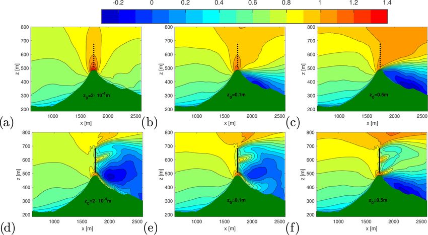
Wind Energ. Sci., 7, 1527–1532, 2022 https://doi.org/10.5194/wes-7-1527-2022N. Troldborg et al.: How does complex terrain change the power curve of a wind turbine? 1529 Figure 1. Power curve of DTU 10 MW turbine in flat (a) and complex (b) terrain as predicted by AD LES and Flex5. Note that the error bars indicating the standard error of the mean are included but are barely visible. Figure 2. Contours of the mean streamwise velocity without (a–c) and with (d–f) the turbine included at different surface roughness levels. The velocities are scaled with the free-stream velocity at the hub position of the wind turbine. To verify this explanation, Fig. 2 shows contours of the and, as shown in Fig. 2f, this causes a weaker wake, leading mean streamwise velocity with and without the turbine in- to lower induction in the rotor plane. Consequently the power cluded for the three cases at wind speeds between 8.5 and increases above the reference power as expected. 9.5 m s−1 , which are highlighted in Fig. 1. These cases As the roughness is decreased the separated region behind mainly differ by their surface roughness, which in effect the ridge becomes smaller and smaller, and eventually the causes a very different free-stream flow field behind the tur- flow becomes nearly attached to the terrain surface. In the bine as seen in Fig. 2a–c. two lower-roughness cases the flow therefore decelerates im- At z0 = 0.5 m there is a large separated region behind the mediately downstream of the turbine, and as seen in Fig. 2d ridge, which acts as a barrier and therefore pushes the flow and e this leads to stronger wakes; hence the power output passing over the hill upwards. As a consequence the free- reduces compared to the flat-terrain counterpart. stream velocity initially accelerates downstream of the rotor, https://doi.org/10.5194/wes-7-1527-2022 Wind Energ. Sci., 7, 1527–1532, 2022
1530                                 N. Troldborg et al.: How does complex terrain change the power curve of a wind turbine?

Figure 3. Free-stream velocity (a) and induced velocity (b) along the centreline of the turbine at different roughness heights. The velocities
are scaled with the free-stream velocity at the position of the wind turbine. The shaded area indicates the standard deviation of the mean. The
vertical dashed line indicates the position of the turbine.

   The strong impact that the flow development in the lee of
                                                                                         16
the ridge has on the wake and induction is consistent with the                           27
                                                                          Cp,max =                ,                                        (3)
findings by Meyer Forsting et al. (2016).                                            (1 − a0 )2
   In order to obtain a more quantitative impression of the
                                                                          which is lower than the Betz limit when a0 < 0.
mechanisms described above, Fig. 3 shows the free-stream
                                                                             Besides the topography itself, our work also shows that the
velocity (U0 ) and induction (U0 − U ) along the centreline
                                                                          power performance is strongly governed by the roughness of
of the turbine for the three cases shown in Fig. 2. The fig-
                                                                          the terrain. Although not investigated in the present work,
ure clearly shows that the induction in the rotor plane corre-
                                                                          we expect that atmospheric stability will also have a very
lates with the level of acceleration/deceleration of the free-
                                                                          strong impact on the performance of the turbine because it
stream velocity downstream of the turbine: a strong deceler-
                                                                          affects the level of separation behind the hill and hence also
ation leads to strong induction and vice versa.
                                                                          the extent to which the wake follows the terrain as shown by
                                                                          Menke et al. (2018).
4   Discussion                                                               The consequence of the above findings is that a site cali-
                                                                          bration may not be sufficient when verifying the power per-
The results presented above show us that the power curves of              formance of turbines in complex terrain. Even in cases where
a turbine in complex and flat terrain may differ significantly            the bias shown here in practice will average out during a full
from each other. Although it may seem surprising at first                 site calibration campaign (due to variations in atmospheric
glance, this is qualitatively in good agreement with the work             stability and wind conditions and seasonal changes in rough-
of Oh and Kim (2015). In addition, there is no contradiction              ness), it is clear that disregarding the downstream develop-
between this finding and some of the theories on diffuser-                ment will lead to increased uncertainties in the power curve
augmented rotors. For example Jamieson (2009) showed that                 verification. In general the power curve of a turbine is site
the theoretical maximum power coefficient of a turbine in a               specific, and hence in principle a performance verification
diffuser is                                                               should be carried out for each individual site or at least a
           16                                                             proper correction should be adopted. This not only pertains
Cp,max =      (1 − a0 ) ,                                        (2)      to turbines in complex terrain but will apply whenever the
           27
                                                                          ambient flow is non-homogeneous, including in wind farms,
where 16/27 is recognized as the Betz limit and a0 is the                 as also shown by Meyer Forsting et al. (2017).
induction parameter due to the diffuser at the position of the
rotor. Since the diffuser produces a speed-up (a0 < 0), Eq. (2)
                                                                          5   Conclusions
predicts an augmented performance of the turbine. However,
in Eq. (2) the power coefficient is based on the undisturbed              The power performance of a DTU 10 MW turbine located in
velocity far upstream, U0 . To express the performance anal-              complex terrain has been studied via large eddy simulations.
ogously to the complex-terrain case, we need to base the                  The simulations revealed that the power curve for the turbine
power coefficient on the free-stream velocity at the position             was significantly different than for the same turbine in flat
of the rotor, i.e. U0 (1−a0 ). In that case the maximum achiev-           homogeneous terrain. The reason for this difference is that
able power coefficient becomes                                            the undisturbed velocity in the region behind the turbine be-
                                                                          comes non-homogeneous at the complex site, and therefore

Wind Energ. Sci., 7, 1527–1532, 2022                                                          https://doi.org/10.5194/wes-7-1527-2022
N. Troldborg et al.: How does complex terrain change the power curve of a wind turbine? 1531
the wake deviates significantly from that generated when the Code and data availability. The simulations are performed using
turbine is operating in flat terrain. Thus, the answer to the proprietary software, but the presented data can be made available
question posed in the title is that if the terrain causes a de- by contacting the corresponding author. The reason that the code is
celeration of the free-stream flow behind the turbine then it not publicly available is that it is research code developed at DTU
leads to underperformance of the turbine, whereas the oppo- that is normally only distributed under licence.
site is true for a downstream flow acceleration. The magni-
tude of the power curve modification depends on how much
Author contributions. NT performed the simulations and drafted
the free-stream flow varies behind the turbine, which again
the article. SJA and AMF contributed to the idea and methodology.
depends on both the roughness and terrain topography. As ELH and SJA performed code validation. SJA, ELH and AMF sup-
a consequence the power curve cannot be seen as a unique ported the analysis and review and edited the manuscript
characteristic of a turbine but will be site specific.
Appendix A: Characteristics of wind turbine inflow Competing interests. The contact author has declared that none
of the authors has any competing interests.
Tables A1 and A2 show some characteristics of the inflow
seen by the wind turbine for each case. The entities in the ta-
bles are the friction velocity u∗ , roughness height z0 , hub ve- Disclaimer. Publisher’s note: Copernicus Publications remains
locity Uhub , turbulence intensity TI, vertical inflow angle θ , neutral with regard to jurisdictional claims in published maps and
shear exponent α and veer φ. Both α and φ are computed institutional affiliations.
from the velocities at lower and upper tip height.
As seen there is a mild sensitivity of the results to friction
velocity for a given roughness. This is unexpected because Acknowledgements. We would like to thank Hans Ejsing Jør-
gensen for leading the project.
the flow should be Reynolds independent. However, it can
be explained by (1) limited effective grid resolution, which
affects the sub-grid-scale turbulence level, and (2) statistical
Financial support. This research has been supported by Ener-
sensitivity, which stems from the fact that the averaging time gistyrelsen (grant no. 64019-0519).
is the same in all cases and therefore the number of flow-
through times varies with friction velocity.
Review statement. This paper was edited by Sandrine Aubrun
Table A1. Inflow characteristics for each case in complex terrain. and reviewed by Javier Sanz Rodrigo and one anonymous referee.
Case u∗ z0 Uhub TI θ α φ
[m s−1 ] [m] [%] [◦ ] [◦ ]
References
1 0.2 2 × 10⁻⁴ 9.3 2.4 1.8 −0.14 0.2
2 0.25 1 × 10⁻¹ 5.9 4.8 5.8 −0.079 2.9
Allen, J., King, R., and Barter, G.: Wind Farm Simu-
3 0.3 1 × 10⁻¹ 7.0 4.6 6.1 −0.076 2.5
lation and Layout Optimization in Complex Terrain, J.
4 0.4 1 × 10⁻¹ 9.4 5.2 5.8 −0.076 2.6
Phys.: Conf. Ser., 1452, 012066, https://doi.org/10.1088/1742-
5 0.45 1 × 10⁻¹ 10.6 5.3 5.6 −0.080 2.7
6596/1452/1/012066, 2020.
6 0.5 1 × 10⁻¹ 11.7 5.5 5.6 −0.079 2.8
Bak, C.: Description of the DTU 10 MW Reference Wind Tur-
7 0.6 1 × 10⁻¹ 14.1 5.9 5.4 −0.079 2.6
8 0.5 5 × 10⁻¹ 8.7 7.0 11.0 −0.015 6.9
bine, Tech. rep., DTU Wind Energy Report-I-0092, Technical
University of Denmark, https://rwt.windenergy.dtu.dk/dtu10mw/
dtu-10mw-rwt (last access: 18 July 2022), 2013.
Berg, J., Troldborg, N., Sørensen, N., Patton, E. G., and Sullivan,
Table A2. Inflow characteristics for each case in flat terrain. P. P.: Large-Eddy Simulation of turbine wake in complex terrain,
J. Phys.: Conf. Ser., 854, 012003, https://doi.org/10.1088/1742-
Case u∗ z0 Uhub TI θ α φ 6596/854/1/012003, 2017.
[m s−1 ] [m] [%] [◦ ] [◦ ] Borraccino, A., Wagner, R., Vignaroli, A., and Meyer Forsting,
A.: Power performance verification in complex terrain
1 0.2 2 × 10⁻⁴ 6.0 4.8 −0.11 0.11 0.22
using nacelle lidars: the Hill of Towie (HoT) cam-
2 0.25 2 × 10⁻⁴ 7.5 5.1 −0.00 0.10 0.31
3 0.3 2 × 10⁻⁴ 9.0 5.2 −0.03 0.10 0.47
paign, no. 158 in DTU Wind Energy E, DTU Wind
4 0.35 2 × 10⁻⁴ 10.5 5.5 −0.01 0.097 0.45 Energy, Denmark, https://orbit.dtu.dk/en/publications/
5 0.4 2 × 10⁻⁴ 12.0 5.6 −0.01 0.097 0.40 power-performance-verification-in-complex-terrain-using-nacelle-l
6 0.5 5 × 10⁻¹ 5.3 13.0 −0.01 0.18 1.6 (last access: 18 July 2022), 2017.
Brodeur, P. and Masson, C.: Numerical site calibration over com-
plex terrain, J. Solar Energ. Eng., 130, 0310201–03102012,
https://doi.org/10.1115/1.2931502, 2008.
https://doi.org/10.5194/wes-7-1527-2022 Wind Energ. Sci., 7, 1527–1532, 20221532 N. Troldborg et al.: How does complex terrain change the power curve of a wind turbine? Castro, I.: Rough-wall boundary layers: Mean Nam, Y., Yoo, N., and Lee, J.: Site calibration for the wind tur- flow universality, J. Fluid Mech., 585, 469–485, bine performance evaluation, KSME Int. J., 18, 2250–2257, https://doi.org/10.1017/S0022112007006921, 2007. https://doi.org/10.1007/BF02990229, 2004. Deardorff, J.: Stratocumulus-capped mixed layers derived from a Oh, H. and Kim, B.: Comparison and verification of the three-dimensional model, Bound.-Lay. Meteorol., 18, 495–527, deviation between guaranteed and measured wind turbine https://doi.org/10.1007/BF00119502, 1980. power performance in complex terrain, Energy, 85, 23–29, Hodgson, E. L., Andersen, S. J., Troldborg, N., Forsting, A. M., https://doi.org/10.1016/j.energy.2015.02.115, 2015. Mikkelsen, R. F., and Sørensen, J. N.: A Quantitative Com- Øye, S.: FLEX4 Simulation of Wind Turbine Dynamics, in: Pro- parison of Aeroelastic Computations using Flex5 and Actu- ceedings of 28th IEA Meeting of Experts Concerning State of the ator Methods in LES, J. Phys.: Conf. Ser., 1934, 012014, Art of Aeroelastic Codes for Wind Turbine Calculations, Lyngby, https://doi.org/10.1088/1742-6596/1934/1/012014, 2021. 1996. Jamieson, P.: Beating betz: Energy extraction limits in a con- Sessarego, M., Shen, W. Z., van der Laan, M. P., Hansen, K. S., and strained flow field, J. Solar Energ. Eng., 131, 0310081–0310086, Zhu, W. J.: CFD simulations of flows in a wind farm in complex https://doi.org/10.1115/1.3139143, 2009. terrain and comparisons to measurements, Appl. Sci. (Switzer- Liu, Z., Lu, S., and Ishihara, T.: Large eddy simulations of wind land), 8, 788, https://doi.org/10.3390/app8050788, 2018. turbine wakes in typical complex topographies, Wind Energy, 24, Shamsoddin, S. and Porté-Agel, F.: Large-Eddy Simulation of 857–886, https://doi.org/10.1002/we.2606, 2021. Atmospheric Boundary-Layer Flow Through a Wind Farm Menke, R., Vasiljević, N., Hansen, K., Hahmann, A., and Mann, J.: Sited on Topography, Bound.-La. Meteorol., 163, 1–17, Does the wind turbine wake follow the topography? A multi- https://doi.org/10.1007/s10546-016-0216-z, 2017. lidar study in complex terrain, Wind Energ. Sci., 3, 681–691, Sørensen, N. N.: General Purpose Flow Solver Applied to https://doi.org/10.5194/wes-3-681-2018, 2018. Flow over Hills, Phd thesis, Risø-R-827(EN), Risø National Meyer Forsting, A., Bechmann, A., and Troldborg, N.: A numerical Laboratory, https://backend.orbit.dtu.dk/ws/portalfiles/portal/ study on the flow upstream of a wind turbine in complex terrain, 12280331/Ris_R_827.pdf (last access: 18 July 2022), 1995. J. Phys.: Conf. Ser., 753, 032041, https://doi.org/10.1088/1742- Yang, X., Pakula, M., and Sotiropoulos, F.: Large-eddy simulation 6596/753/3/032041, 2016. of a utility-scale wind farm in complex terrain, Appl. Energy, Meyer Forsting, A., Troldborg, N., and Gaunaa, M.: The flow 229, 767–777, https://doi.org/10.1016/j.apenergy.2018.08.049, upstream of a row of aligned wind turbine rotors and 2018. its effect on power production, Wind Energy, 20, 63–77, https://doi.org/10.1002/we.1991, 2017. Wind Energ. Sci., 7, 1527–1532, 2022 https://doi.org/10.5194/wes-7-1527-2022
You can also read