Breakfast Canyon Discovered in Honeybee Hive Weight Curves - MDPI
←
→
Page content transcription
If your browser does not render page correctly, please read the page content below
insects
Article
Breakfast Canyon Discovered in Honeybee Hive
Weight Curves
Niels Holst 1, *      and William G. Meikle 2
 1   Department of Agroecology, Aarhus University, Forsøgsvej 1, 4200 Slagelse, Denmark
 2   Carl Hayden Bee Research Center, 2000 E Allen Rd, Tucson, AZ 85719, USA;
     William.Meikle@ARS.USDA.GOV
 *   Correspondence: niels.holst@agro.au.dk; Tel.: +45-22-28-33-40

 Received: 9 October 2018; Accepted: 24 November 2018; Published: 1 December 2018

 Abstract: Electronic devices to sense, store, and transmit data are undergoing rapid development,
 offering an ever-expanding toolbox for inventive minds. In apiculture, both researchers and
 practitioners have welcomed the opportunity to equip beehives with a variety of sensors to monitor
 hive weight, temperature, forager traffic and more, resulting in huge amounts of accumulated data.
 The problem remains how to distil biological meaning out of these data. In this paper, we address the
 analysis of beehive weight monitored at a 15-min resolution over several months. Inspired by an
 overlooked, classic study on such weight curves we derive algorithms and statistical procedures to
 allow biological interpretation of the data. Our primary finding was that an early morning dip in the
 weight curve (‘Breakfast Canyon’) could be extracted from the data to provide information on bee
 colony performance in terms of foraging effort. We include the data sets used in this study, together
 with R scripts that will allow other researchers to replicate or refine our method.

 Keywords: monitoring; time series; analysis; segmented linear regression; diurnal; neonicotinoid

1. Introduction
     In 1922 Hambleton [1] assigned laborers the task of measuring the weight of two beehives over
several months at precise hourly intervals, continuously, day and night. The high-precision scales
(±10 g) yielded a unique insight into the daily pattern of hive weight change, resulting from the
interplay between the honeybee colony and its surroundings. Hambleton [1] identified a pattern which
he summarized in a graph, displaying a series of line segments with clearly defined shifts in slope
(Figure 1). After sunrise he found a ‘morning loss’ (from A to B) interpreted as the recruitment of
foragers. The morning loss would end abruptly as foragers began returning, thus creating a steady rate
of net gain (B to D) due to incoming nectar. He acknowledged that the course of weight change from
B to D would vary according to weather and the availability of nectar sources. Between sunset and
sunrise (from D to E) he found a constant ‘nocturnal loss’ rate attributed to evaporation and respiration.
     The within-day dynamics of beehive weight was not studied further until 70 years later when
Buchmann and Thoenes [2] repeated the procedure of Hambleton [1], albeit using electronic scales
linked to data loggers. Without recognizing the precedence in Hambleton’s work, they identified the
same daily pattern during nectar flows as seen in Figure 1. Later, Meikle et al. [3–5] analyzed more
extensive data sets of continuously monitored beehive weight but daily variation was reduced to a
simple sine wave curve without going into any details of the daily pattern.

Insects 2018, 9, 176; doi:10.3390/insects9040176                              www.mdpi.com/journal/insects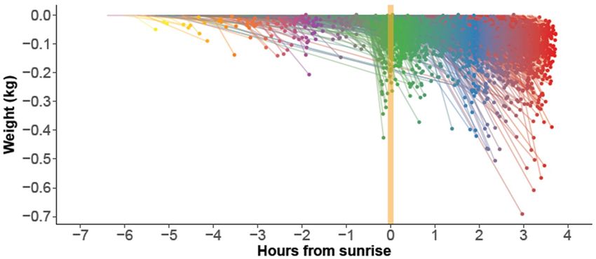
Insects 2018, 9, 176 2 of 11
Insects 2018, 9, x FOR PEER REVIEW 2 of 11
Figure1.1.Hambleton’s
Figure Hambleton’s Graph
Graph [1]
[1] with
with Breakfast
Breakfast Canyon
Canyon added
added shows
showsthe
thedaily
dailypattern
patternofofbeehive
beehive
weight during a nectar flow. Abrupt changes in slope occur at A, B, D and E. The canyon has adepth
weight during a nectar flow. Abrupt changes in slope occur at A, B, D and E. The canyon has a depth
(kg)equal
(kg) equaltotothe
theweight
weightatatAAminus
minusthe
the weight
weight at
at B.
B.
Thework
The workpresented
presentedhereherebegan
beganasaswe wewere
wereintrigued
intriguedby byaaregular
regularpattern
patternfound
foundininthe
theweight
weightof
of continuously monitored beehives in Southern Arizona. On many mornings,
continuously monitored beehives in Southern Arizona. On many mornings, there would be a distinct there would be a
distinct dip in weight. This we dubbed ‘Breakfast Canyon’ after a nearby locality,
dip in weight. This we dubbed ‘Breakfast Canyon’ after a nearby locality, only later realizing that the only later realizing
that thelow
canyon canyon
pointlow point corresponded
corresponded to the pointto the point
B of B of Hambleton
Hambleton (Figure 1).(Figure 1).
Continuous weight curves logged at a frequency of
Continuous weight curves logged at a frequency of 1 h or less is one 1 h or less is oneofof several
several measures
measures used
used for
for automatic monitoring of beehive status [6]. If the hive resides constantly
automatic monitoring of beehive status [6]. If the hive resides constantly on a scale, this monitoring on a scale, this
monitoring method is nonintrusive. The logged readings of total hive weight are directly linked to
method is nonintrusive. The logged readings of total hive weight are directly linked to the accumulation
the accumulation of honey and pollen stores, which is an important measure of bee colony
of honey and pollen stores, which is an important measure of bee colony performance. In addition, the
performance. In addition, the daily amplitude of weight change has been used to infer bee colony
daily amplitude of weight change has been used to infer bee colony size [4,5]. Recently, the within-day
size [4,5]. Recently, the within-day pattern of weight changes was analyzed using segmented linear
pattern of weight changes was analyzed using segmented linear regression [7]. It was concluded that
regression [7]. It was concluded that the early morning weight loss was mostly due to foragers
the early morning weight loss was mostly due to foragers leaving.
leaving.
Here we will address three questions: (i) Is it possible to extract consistently the salient features of
Here we will address three questions: (i) Is it possible to extract consistently the salient features
Hambleton’s Graph from beehive weight curves? Are the extracted parameters useful for (ii) describing
of Hambleton’s Graph from beehive weight curves? Are the extracted parameters useful for (ii)
honeybee colony behavior and for (iii) diagnosing neonicotinoid stress? Of these questions, the first two
describing honeybee colony behavior and for (iii) diagnosing neonicotinoid stress? Of these
explores thethe
questions, quality andexplores
first two usefulnesstheof the extracted
quality parameters,
and usefulness of thewhile the last
extracted one forms
parameters, a hypothesis
while the last
that can be rigorously tested.
one forms a hypothesis that can be rigorously tested.
We
Weused
usedtwo twoearlier-published
earlier-publisheddatadata sets
sets [4]
[4] for the analysis
for the analysisfrom
fromwhich
whichwe weestimated
estimatedthree
threedaily
daily
parameter values for each beehive: (1) nocturnal loss rate (kg/h), (2) depth of
parameter values for each beehive: (1) nocturnal loss rate (kg/h), (2) depth of Breakfast Canyon (kg) Breakfast Canyon (kg)
(Figure 1), and (3) daily weight gain (kg/d). Questions (i) and (ii) were explored
(Figure 1), and (3) daily weight gain (kg/d). Questions (i) and (ii) were explored graphically while for graphically while
for question
question (iii)
(iii) thethe three
three parameters
parameters were
were used
used asasresponse
responsevariables,
variables,regressed
regressed uponthe
upon thelevel
levelofof
neonicotinoid stress brought upon the honeybees in the experiments [4].
neonicotinoid stress brought upon the honeybees in the experiments [4]. The three parameters wereThe three parameters were
successfully extracted by a common
successfully extracted by a common R script R script and provided detailed information on honeybee
provided detailed information on honeybee colony colony
behavior,
behavior,iningeneral,
general,asaswell
wellasasunder
underneonicotinoid
neonicotinoid stress.
stress.
2. Materials and Methods
2.1. Beehive Data Sets
Details of the two experiments that generated the data used in this paper are described elsewhere
[4]. Both data sets originate from experiments conducted in the desert climate near Tucson, Arizona,
Insects 2018, 9, 176                                                                               3 of 11

2. Materials and Methods

2.1. Beehive Data Sets
      Details of the two experiments that generated the data used in this paper are described
elsewhere [4]. Both data sets originate from experiments conducted in the desert climate near Tucson,
Arizona, USA to assess the effect of a neonicotinoid insecticide (imidacloprid) supplied regularly in
syrup fed to the bees. Hive weights were monitored continuously at 15-min intervals.
      The first data set (2014) encompassed 12 beehives for the period 20 April to 17 November 2014.
Treatments began 15 July with control (0 ppb), low (5 ppb) and high (100 ppb) doses of insecticide fed
in 1:1 sugar syrup with four beehives in each treatment group. The second data set (2015) encompassed
16 beehives for the period 2 May to 14 August 2015. Treatments began 10 July with control (0 ppb),
low (5 ppb), medium (20 ppb) and high (100 ppb) doses of insecticide, again with four beehives in
each treatment group. In the 2015 data set, data from one medium treatment hive were discarded due
to wild animal disruption. The experiment as a whole was cut short due to robbery by a black bear.

2.2. Data Preparation
     Data from dates when the hives had been manipulated (e.g., by feeding or hive inspection) were
discarded from the analysis. Likewise, dates with unexplained, sudden gains in weight were discarded;
presumably these were days with heavy rainfall. A few abrupt changes in weight remained, usually due
to the checking of equipment; data from these hive × date instances were also discarded. The logged
weight was sometimes punctuated by aberrant readings: one or two readings clearly disjoint from
readings before and after. These instances were detected algorithmically by the magnitude of weight
change, both relatively (kg/h) and absolutely (kg) (see details in the noise_drop function found in the
bc-general.R script in File S2). The disjoint readings were considered missing values. The time stamp of
all measurements was transformed from local time to solar time by which solar noon coincides with
12:00; the same algorithm [8] was used to estimate the time of sunrise.

2.3. Parameter Estimation
     The whole procedure described in the following was automatized in an R script (available
in File S2). To describe the daily weight pattern, we used the segmented linear regression (SLR)
procedure found in the R package ‘segmented’ [9]. SLR estimates n linear regression lines, joined at
n − 1 breakpoints. An SLR with n = 4 segments was carried out for each hive × instance separately
on data from midnight to 4 h after sunrise. The ‘segmented’ package uses a stochastic method to
search for a solution and thus will not always give the same outcome. Therefore, the analysis was
replicated n = 30 times. If the analysis failed all N times, we tried again with n = 60, then n = 120 and
lastly n = 240 times. If no solution was found then the analysis was abandoned for that hive × date
instance. Usually more than one solution was found, in which case the solution with the highest r2 was
chosen. Examples of the estimated SLR models are shown in Figure 2. The same procedure, just with
n = 3 segments, was also carried out but failed to detect many Breakfast Canyon instances obvious to
the eye (results not shown).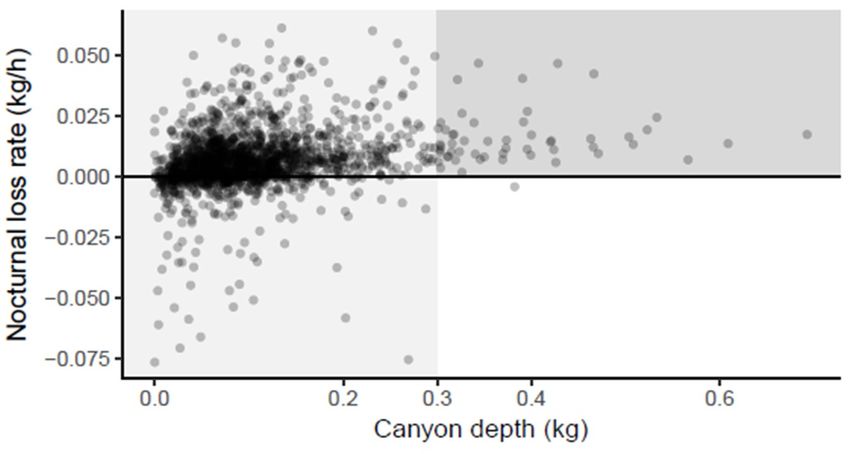
Insects 2018, 9, 176 4 of 11
Insects 2018, 9, x FOR PEER REVIEW 4 of 11
p
Figure 2. Typical course of the segmented linear regression (SLR) models. For each of the 15 types, the
Figure 2. Typical course of the segmented linear regression (SLR) models. For each of the 15 types,
model with the median r2 value was selected as typical and shown above, identified by date and hive
the model with the median r2 value was selected as typical and shown above, identified by date and
number. The four segments are shown in different colours while the underlying black curve shows the
hive number. The four segments are shown in different colours while the underlying black curve
weight during 24 h. Light vs. dark background shows day vs. night. The inset graphical keys refer
shows the weight during 24 h. Light vs. dark background shows day vs. night. The inset graphical
to Figure 3.
keys refer to Figure 3.
For each hive × date instance, the SLR model was evaluated for concordance with the Hambleton
For each hive × date instance, the SLR model was evaluated for concordance with the Hambleton
diagram (Figure 1): An SLR was considered a Breakfast Canyon (BC) SLR, if one of the line segments
diagram (Figure 1): An SLR was considered a Breakfast Canyon (BC) SLR, if one of the line segments
with a negative slope was followed by one with a positive slope, constituting the two line segments
with a negative slope was followed by one with a positive slope, constituting the two line segments
A-B and B-D in Hambleton’s Graph (Figure 1). These could be segments 2-3 or 3-4 but not 1-2, because
A-B and B-D in Hambleton’s Graph (Figure 1). These could be segments 2-3 or 3-4 but not 1-2, because
segment
segment 1 starts at at
1 starts midnight
midnight (ruling
(rulingoutout
that thethe
that canyon
canyon could
couldcommence
commence at midnight).
at midnight). In the
In the3-43-4
case,
segment 2 could2possibly
case, segment have a negative
could possibly slope even
have a negative slopesteeper than segment
even steeper 3, indicating
than segment that segment
3, indicating that
2 formed
segment 2 formed the true onset of the canyon. If so, segments 2-3-4 formed the canyonbottom
the true onset of the canyon. If so, segments 2-3-4 formed the canyon with the with the still
between segment 3-4.
bottom still between segment 3-4.
For every
For every BCBCSLRSLRmodel,
model,thethe
nocturnal
nocturnal loss rate
loss (kg/h)
rate (kg/h)was
wasestimated
estimatedasasthe thenegative
negativeslopeslopeofofthe
longest segment ending at the rim of Breakfast Canyon (point A in Figure 1) or
the longest segment ending at the rim of Breakfast Canyon (point A in Figure 1) or earlier. Canyon earlier. Canyon depth
(kg) was(kg)
depth estimated according
was estimated to Figureto1.Figure
according For hive × date
1. For hiveinstances that hadthat
× date instances no BChadSLR,
no BCtheSLR,
nocturnal
the
loss rate andloss
nocturnal canyon depth
rate and weredepth
canyon considered missing. missing.
were considered
ToTo estimatethe
estimate theweight
weight atat midnight,
midnight, aaparabolic
paraboliccurve
curvewaswas fitfit
bybylinear regression
linear regressionto the
to data at
the data
at midnight ±1 h. This resulted in a robust interpolation of weight at 24:00; however, if less than
midnight ±1 h. This resulted in a robust interpolation of weight at 24:00; however, if less than three
observations
three werewere
observations available in theininterval
available then weight
the interval at midnight
then weight was considered
at midnight was consideredmissing. The
missing.
weight
The weightgain (kg/d)
gain (kg/d)forfor
a particular
a particularhive
hive× date
× dateinstance
instancewaswasfound
found as as
thethe
increase
increasein in
thethe
estimated
estimated
midnight
midnight weightfrom
weight fromoneonemidnight
midnightto tothe
thenext.
next.
2.4.
2.4. StatisticalAnalysis
Statistical Analysis
TheThequality
qualityofofthe
theestimated
estimated nocturnal
nocturnal loss rates
rates and
and canyon
canyondepths
depthswas
wasverified
verifiedvisually
visuallybyby
plotting the corresponding extracted line segments. Any line segments with unrealistically
plotting the corresponding extracted line segments. Any line segments with unrealistically steep slopes steep
slopes
were were identified
identified and discarded
and discarded fromofthe
from the rest therest of the The
analysis. analysis. The between
relations relationsthe
between the three
three parameters
parameters
(nocturnal loss(nocturnal lossdepth
rate, canyon rate, canyon depth
and weight andwere
gain) weight gain) were
explored explored
in three pairwisein scatterplots
three pairwise
with
the aim to hypothesize on plausible explanations for any patterns found. This explorativefound.
scatterplots with the aim to hypothesize on plausible explanations for any patterns This
analysis was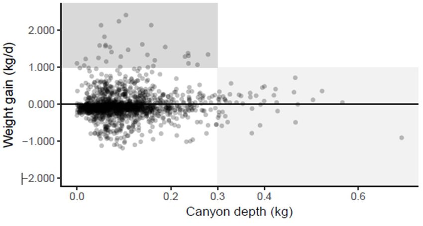
Insects 2018,
Insects 2018, 9,
9, 176
x FOR PEER REVIEW 55 of
of 11
11
explorative analysis was followed by a formal statistical procedure to test if the level of neonicotinoid
followed
stress hadbyana impact
formal on
statistical procedure
any of the to test if the level of neonicotinoid stress had an impact on
three parameters.
any ofWe
theapplied
three parameters.
a linear mixed model, once for each of the 3 parameters for each year; a total of 6
We applied
analyses. a linear
The model was mixed model,
formulated in Ronce
usingforthe
each of function:
‘lme’ the 3 parameters for each year; a total of
6 analyses. The model was formulated in R using the ‘lme’ function:
lme(fixed = Parameter ~ Treatment ∗ Period, random = ~Date|Hive,
correlation
lme(fixed = Parameter ∼ = corCAR1(form
Treatment = ~Date|Hive))
∗ Period, random =∼ Date|Hive,
where Parameter designates one of the three parameters (Breakfast Canyon depth, daily
correlation = corCAR1(form =∼ Date|Hive))
weight gain or nocturnal loss rate), Treatment had 3 levels in 2014 and 4 levels in 2015, and
wherePeriod had 2designates
Parameter levels designating before
one of the threeor after the onset
parameters of theCanyon
(Breakfast neonicotinoid
depth, treatment for gain
daily weight
that year.
or nocturnal lossThe random
rate), argument
Treatment tells that
had 3 levels Hiveand
in 2014 is 4the subject
levels repeated
in 2015, by Date.
and Period hadThe
2 levels
correlation argument specifies the autocorrelation model, which estimated the correlation
designating before or after the onset of the neonicotinoid treatment for that year. The random argument
coefficient
tells that Hive is(ϕ)
thebetween model residuals
subject repeated by Date.1Thedaycorrelation
apart. Additional
argumentdetails are given
specifies in File S1:
the autocorrelation
Section 1.
model, which estimated the correlation coefficient (φ) between model residuals 1 day apart. Additional
details are given in File S1: Section 1.
3. Results
3. Results
After discarding data from dates disturbed by rain and hive manipulations, a total of 3750 hive
× date instances
After remained
discarding (2014:dates
data from 2204,disturbed
2015: 1546). The and
by rain segmented regression procedure
hive manipulations, a total of successfully
3750 hive ×
estimated
date 3742remained
instances 4-segmented
(2014:SLRs.
2204,Thus, it failed
2015: 1546). Theinsegmented
only eight regression
cases. However,
procedurefor successfully
some of the
estimated SLRs,
estimated the nocturnalSLRs.
3742 4-segmented loss rate wasitimpossibly
Thus, failed in onlylarge. By experimentation,
eight cases. However,afor threshold
some ofofthe 3.4
s.d. from the
estimated average
SLRs, was found
the nocturnal losstorate
detect
wasthese cases. The
impossibly large.detected 15 hive × dateainstances
By experimentation, thresholdhad a loss
of 3.4 s.d.
>97 g/h
from theoraverage
a gain >84
wasg/h, both
found to unlikely
detect theseto occur at The
cases. night. They were
detected removed,
15 hive × datereducing
instancesthehaddata set
a loss
finally to 3727 instances. Typical examples of the 3727 SLR models are shown in
>97 g/h or a gain >84 g/h, both unlikely to occur at night. They were removed, reducing the data set Figure 2.
Depending
finally on the Typical
to 3727 instances. course of the segments
examples (Figure
of the 3727 SLR 3), 1904 are
models of the 3727
shown in SLRs
Figure(51%)
2. allowed
estimation
Dependingof canyon
on thedepth
courseand thereby
of the nocturnal
segments (Figureloss rate as
3), 1904 of well. TheSLRs
the 3727 remaining 3727 − 1904
(51%) allowed = 1823
estimation
SLRs,
of for which
canyon a Breakfast
depth and thereby Canyon
nocturnalfeature could
loss rate not be
as well. Theidentified,
remainingwere3727dominated
− 1904 = 1823by segments
SLRs, for
with negative
which a Breakfastslopes (Figure
Canyon 3); i.e.,
feature couldlosses
not persisted fromwere
be identified, the dominated
night until by
4 hsegments
after sunrise
withwhen the
negative
analysis ended.
slopes (Figure 3); i.e., losses persisted from the night until 4 h after sunrise when the analysis ended.
Figure 3. The 15 types of SLR models that best described the weight curves with each type characterized
Figure 3. The 15 types of SLR models that best described the weight curves with each type
by a sequence of positive and negative slopes. The number found of each type is shown. Breakfast
characterized by a sequence of positive and negative slopes. The number found of each type is shown.
Canyon segments are shown in red—in some cases (a: 174; b: 35) it was extended by one segment to
Breakfast Canyon segments are shown in red—in some cases (a: 174; b: 35) it was extended by one
the left (not shown in red).
segment to the left (not shown in red).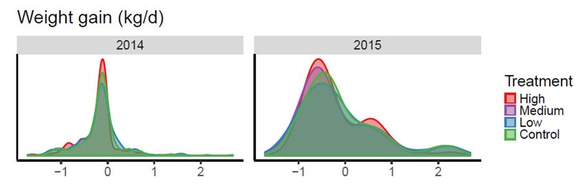
Insects 2018, 9, 176 6 of 11
Insects 2018, 9, x FOR PEER REVIEW 6 of 11
The nocturnal loss segments had mostly negative slopes indicating, indeed, a weight loss (Figure 4
The nocturnal loss segments had mostly negative slopes indicating, indeed, a weight loss (Figure
top). Weight gains during the night caused by rain had been filtered out before the analysis, so the
4 top). Weight gains during the night caused by rain had been filtered out before the analysis, so the
instances of slight nightly weight gains must have other explanations, maybe light rains or moisture
instances of slight nightly weight gains must have other explanations, maybe light rains or moisture
uptake from the air.
uptake from the air.
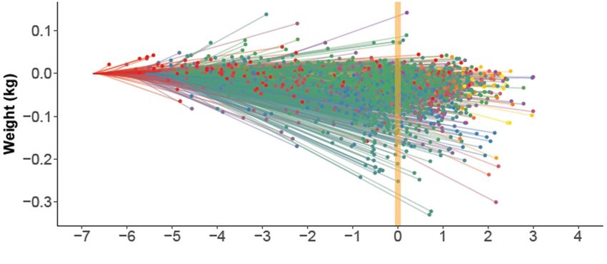
The onset of Breakfast Canyon (point A in Figure 1) mostly occurred at 12 hour before sunrise
The onset of Breakfast Canyon (point A in Figure 1) mostly occurred at ½ hour before sunrise or
or later (Figure 4 bottom). Canyon bottoms (point B in Figure 1) reached in this interval were also
later (Figure 4 bottom). Canyon bottoms (point B in Figure 1) reached in this interval were also the
the deepest.
deepest.
Figure 4. Extracted line segments (n =
= 3727)
3727) used to estimate nocturnal
nocturnal loss rate (top) and Breakfast
Canyon depth (bottom).
(bottom). They
They correspond
correspond to
to lines
lines D-E
D-E and
and A-B,
A-B, respectively, in Hambleton’s Graph
(Figure 1). All segments were translated to begin at zero weight. Line segments and endpoints were
color-coded according to the hour of the segment’s beginning to aid
aid the
the visualization.
visualization.
The scatter
scatter plots
plotsofofthe
thethree
threeestimated
estimated parameters
parameters were inspected
were inspectedfor visual patterns
for visual whichwhich
patterns were
highlighted
were by background
highlighted by background shading (Figure
shading 5). As5).these
(Figure patterns
As these were were
patterns inspired by the
inspired bydata, they
the data,
cannot
they undergo
cannot statistical
undergo hypothesis
statistical testing but
hypothesis onlybut
testing serve to develop
only serve to plausible
develop biological
plausible inferences
biological
and hypotheses.
inferences and hypotheses.
A deep Breakfast Canyon (>0.3 (>0.3 kg)
kg) was
was never
never followed
followed by by a large daily weight gain (>1 (>1 kg)
kg)
(Figure 5 top, light shading). This could be the the result
result of foragers,
foragers, which
which on on days
days with
with scarce
scarce resources
resources
would spend more time scouting, thus extending and deepening the canyon before they returned
with empty
emptycrops.
crops.InIn contrast,
contrast, shallow
shallow canyons
canyons (depth
(depth < 0.30.3(>0.3 kg)
kg) only
only occurred
occurredafterafternights
nightswith
withaadistinct
distinctweight
weightloss
loss(Figure
(Figure5
middle, dark shading). If the weight loss was caused by drying nectar, foragers
5 middle, dark shading). If the weight loss was caused by drying nectar, foragers might have been might have been cued
to leave
cued in high
to leave in numbers
high numbersanticipating yet another
anticipating day ofday
yet another highof nectar flow. flow.
high nectar
The nocturnal loss rate was always high when the weight gain during the previous day had been
large (>0.6 kg) (Figure 4 bottom, dark shading right). This would be expected since most of the gain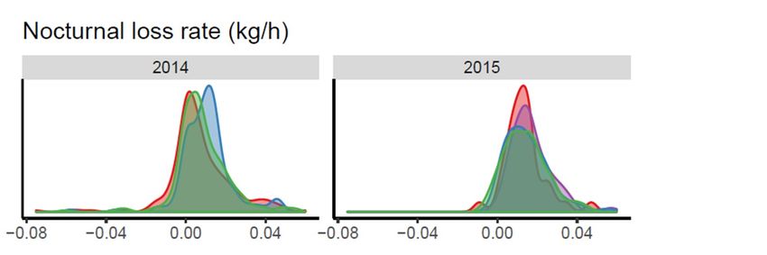
Insects 2018, 9, 176                                                                                             7 of 11

       The nocturnal loss rate was always high when the weight gain during the previous day had7been
Insects 2018, 9, x FOR PEER REVIEW                                                                               of 11
large (>0.6 kg) (Figure 4 bottom, dark shading right). This would be expected since most of the gain
would be
would     be due
             due to
                  tonectar,
                      nectar,the
                              themain
                                   mainsource
                                         sourceforfor
                                                    evaporation
                                                      evaporationduring  thethe
                                                                    during   night.  However,
                                                                                 night.  However,a tremendous
                                                                                                      a tremendousloss
the  day   before  (more  than  1 kg), as well led  to high losses at night (Figure  4 bottom,   dark
loss the day before (more than 1 kg), as well led to high losses at night (Figure 4 bottom, dark shadingshading  left).
Apparently,
left).          thesethese
       Apparently,     hiveshives
                              suffered  a sustained
                                    suffered           weight
                                             a sustained       loss loss
                                                            weight  fromfrom
                                                                          the previous    dayday
                                                                               the previous    thatthat
                                                                                                     lasted  intointo
                                                                                                          lasted   the
night.
the      For For
     night.   intermediate   weight
                   intermediate       gainsgains
                                  weight    during   the day
                                                   during  the(Figure 4 bottom,
                                                                day (Figure       light shading),
                                                                             4 bottom,             rates of rates
                                                                                          light shading),    gains of
                                                                                                                    as
well   as losses  occurred  the  following  night.
gains as well as losses occurred the following night.

      Figure
      Figure 5.
              5. Scatter
                 Scatter plots
                         plots of
                               of parameter
                                  parameter values
                                              values estimated  for each
                                                     estimated for  each hive
                                                                         hive ×× date
                                                                                 date instance
                                                                                       instance (n
                                                                                                (n ==3732).
                                                                                                     3732). Weight
                                                                                                            Weight
      gain is shown   either for  the
      gain is shown either for the samesame  day (top) or for the day before  (bottom).  Light  and  dark  shading
                                                                                          Light and dark shading
      shows
      shows patterns
              patterns explained
                        explained inin text.

     When the three parameters were applied as response variables for the neonicotinoid treatments
(Figure 6), the treatment with the highest concentration pushed the distribution towards lower values
for Breakfast Canyon depth, making it shallower. The statistical treatment (see File S1: Section 1)
supported this result (p = 0.003 for both years). The other two parameters seemed not to react to the
treatment.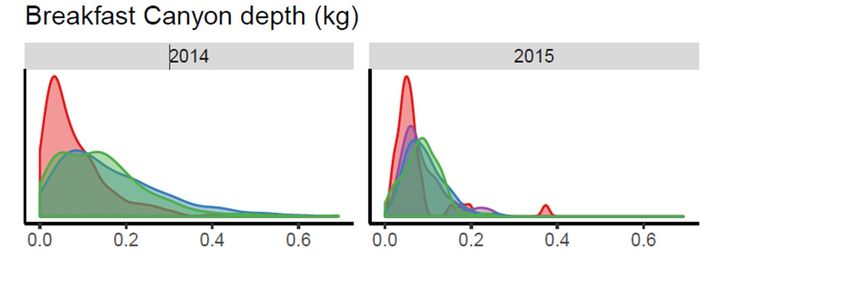
Insects 2018, 9, 176                                                                                            8 of 11

       When the three parameters were applied as response variables for the neonicotinoid treatments
(Figure 6), the treatment with the highest concentration pushed the distribution towards lower values
for Breakfast Canyon depth, making it shallower. The statistical treatment (see File S1: Section 1)
supported this result (p = 0.003 for both years). The other two parameters seemed not to react to
the  treatment.
 Insects 2018, 9, x FOR PEER REVIEW                                                             8 of 11

      Figure 6.6. Density
      Figure      Density plots
                            plots of
                                  of daily
                                     daily parameter
                                           parameter values
                                                     values estimated
                                                            estimated in
                                                                      in the
                                                                         the period
                                                                             period after
                                                                                     after pesticide
                                                                                           pesticide treatment.
                                                                                                     treatment.
      The
      The area under each curve equals one. In 2014 there was no medium treatment. Formal statistics
          area   under   each  curve  equals one. In 2014 there was no medium    treatment.   Formal   statistics
      presented
      presentedin  inFile
                      FileS1:
                           S1:Section
                              Section1.1.
4. Discussion
 4. Discussion
      The obvious statistic to extract from beehive weight curves is the daily weight gain e.g., [10,11].
      The obvious statistic to extract from beehive weight curves is the daily weight gain e.g., [10,11].
Easily calculated as the weight difference between subsequent midnights, it is directly related to
 Easily calculated as the weight difference between subsequent midnights, it is directly related to the
the hoarding of honey and therefore relevant both to the understanding of honeybee ecology and
 hoarding of honey and therefore relevant both to the understanding of honeybee ecology and to
to monitoring of honeybee colony performance. However, through segmented linear regression
 monitoring of honeybee colony performance. However, through segmented linear regression and
and subsequent algorithmic analysis, we successfully extracted more detailed information from the
 subsequent algorithmic analysis, we successfully extracted more detailed information from the daily
daily weight curves, ultimately obtaining consistent estimates of two features of Hambleton’s Graph
 weight curves, ultimately obtaining consistent estimates of two features of Hambleton’s Graph
(Figure 1), namely nocturnal loss rate and Breakfast Canyon (BC) depth.
 (Figure 1), namely nocturnal loss rate and Breakfast Canyon (BC) depth.
      The weight changes of a beehive result as a summation of several concurrent processes: nectar
      The weight changes of a beehive result as a summation of several concurrent processes: nectar
inflow and evaporation, fluctuations in honey and pollen stores, base and heating respiration, worker
 inflow and evaporation, fluctuations in honey and pollen stores, base and heating respiration, worker
mortality, precipitation, dew, and physical exchanges of humidity between the air and the beehive
 mortality, precipitation, dew, and physical exchanges of humidity between the air and the beehive
construction. Pollen stores tend to be short-lived and are not usually stockpiled during periods of
 construction. Pollen stores tend to be short-lived and are not usually stockpiled during periods of
 ample pollen resources [12,13]. Hence, pollen collection effort is driven by the current demand of the
 brood [14] and by its availability; the collected pollen is readily consumed. Nectar, on the other hand,
 is collected both to cover the current energetic demands of the colony and to process and store as
 honey. This is the basis for ‘nectar flows’, i.e., periods with a steady increase in honey stores. Overall,
 colonies usually recruit more foragers for nectar collection than for pollen collection [14].
Insects 2018, 9, 176                                                                                  9 of 11

ample pollen resources [12,13]. Hence, pollen collection effort is driven by the current demand of the
brood [14] and by its availability; the collected pollen is readily consumed. Nectar, on the other hand, is
collected both to cover the current energetic demands of the colony and to process and store as honey.
This is the basis for ‘nectar flows’, i.e., periods with a steady increase in honey stores. Overall, colonies
usually recruit more foragers for nectar collection than for pollen collection [14].
     Hambleton [1] expected his graph (Figure 1) to apply only to periods of nectar flow. In our study,
we identified his graph by a distinctive BC which we found in 51% of the cases. Since we consider
nectar flows to have been present less than 20% of the time, Hambleton’s Graph seems applicable also
outside nectar flows.
     Base respiration will, in general, change only slowly as the colony changes in size and distribution
among life stages. In the desert climate of the experiments reported here, respiration must have
risen every night to maintain hive temperature in face of the cold outdoors. Total respiration rates
of 30−50 g/day have been reported from beehives overwintered at 3–5 ◦ C [15]; we would expect
these respiration rates to apply roughly to our hives a well. Water carried in by the bees to cool the
hive would not register on the scale, as water is not stored but brought to evaporation immediately.
Rain was a rare event but major rainfall events could be detected and were removed from the data set
to reduce noise. Thus, disregarding minor showers and physical changes of humidity, major weight
changes in these experiments must have been caused by honeybee traffic, together with nectar inflow
and its transformation into honey, which involves water evaporation.
     The proportion of a bee colony that are foragers varies from 4.1% to 9.6%—larger during nectar
flows [16]. The average weight of a worker honeybee has been reported at 115 mg [17] and 128 mg [3].
BC depth varied (Figure 5 top) with a median value of 85 g and a 95% percentile of 249 g. Assuming an
average weight of 122 mg for a bee, we get a median BC depth corresponding to 85/0.122 = 697 bees
and a 95% percentile of 249/0.122 = 2041 bees. Assuming further that the 95% percentile applies to
nectar flow periods, we get an estimate of the total colony size of 2041/0.096 = 21,260 bees. If the
median BC depth applies to non-nectar flow periods, which were dominant during the observation
periods, we get a total of 697/0.041 = 17,000 bees. The adult bee population in these experiments was
typically in the 2–4 kg range [4], corresponding to a colony size of 16,400–32,800 bees (122 mg per bee).
Thus, the estimated BC depths are consistent with the hypothesis that BC was caused by bees leaving.
     The mechanisms connecting daily weight gain, nocturnal loss rate and BC depth (Figure 5) were
interpreted in terms of honeybee biology. Nocturnal weight gains were not unusual. This points to
moisture taken up by the hive structure (made of wood) and by open pollen and nectar cells during
the desert night when the relative humidity of the air is rising. In Southern France, empty wooden
hives will fluctuate as much as 200 g in weight between night and day [18]; however, in an occupied
beehive the fluctuation will likely be less due to the microclimate-regulating habit of the honeybees.
     Scout bees will return and recruit foragers through their waggle dance, probably resulting on any
given day in a focus on a few high-yielding patches [19]. A potential forager will instead become a
scout, the longer time it waits without meeting a recruiting (dancing) bee [20]. In the event that a food
patch persists, foragers are likely to remember this and will continue to exploit the same patch without
further scouting [21]. These mechanisms will make scouts and foragers out of most of the honeybees
leaving during the BC period. If abundant resources are found nearby, the bees will return quickly.
This will lead to a shallow BC and a high weight gain on the same day. This mechanism was supported
by our data, in which a deep BC never coincided with a high weight gain (Figure 5 top, light shading).
     In the original paper [4] presenting the data reused here, it was found that the ‘high’ neonicotinoid
treatment reduced both colony size and average frame weight. We found a reduced BC depth for
the high treatment (Figure 6 and statistical analysis in File S1: Section 1), which indicates a lowered
foraging capacity of the bee colony. This result supports the original conclusion, that bee colonies were
weakened by the high treatment. In conclusion, BC depth might represent a new measure by which to
monitor bee colony strength.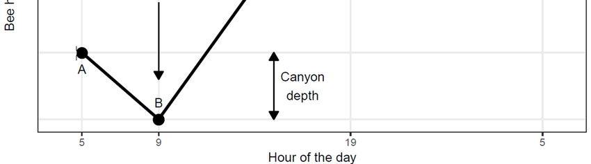
Insects 2018, 9, 176                                                                                           10 of 11

      We successfully estimated segmented linear regressions in agreement with Hambleton’s Graph
(Figure 1) even outside nectar flows. The shape of this graph, however, may vary among climates.
Cooler mornings would delay the onset of Breakfast Canyon. A colony placed near a superabundant
nectar resource, such as a commercial field of oilseed rape, might shorten the foraging trip as much as
to fill up the Breakfast Canyon with returning scouts and foragers, so fast that the canyon would not
show; its detection relies on a delay until the first successful bees return.
      In rainy locations, it might be difficult to achieve an undisturbed time series of hive weight.
For hives not in some kind of shelter, foraging activity between rain showers would be difficult to
filter out from weight fluctuations due to the accumulation of rain on the hive and subsequent drying.
For research purposes, the hive and scale should be protected by a rain cover. In addition, hives made
of water-inert materials, such as plastic foam, would reduce the noise produced by fluctuations in hive
moisture content.
      The collection of a variety of sensor data (weight, temperature, humidity, acoustics, digital vision)
from honeybee hives has received much attention recently [6]. However, there is a lack of methods to
turn the accumulated body of data into biologically meaningful information. The method described
here is a step towards establishing a toolbox to turn beehive sensor data into valuable research and
monitoring information.

Supplementary Materials: The following are available online at http://www.mdpi.com/2075-4450/9/4/176/s1,
File S1: Application and R script documentation, File S2: R scripts and input files.
Author Contributions: Conceptualization, N.H. and W.G.M.; Methodology, N.H. and W.G.M.; Software, N.H.;
Validation, N.H.; Formal Analysis, N.H.; Investigation, N.H. and W.G.M.; Resources, W.G.M.; Data Curation,
N.H. and W.G.M.; Writing–Original Draft Preparation, N.H.; Writing–Review & Editing, N.H. and W.G.M.;
Visualization, N.H.
Funding: This research received no external funding.
Acknowledgments: Niels Holst was supported by a fellowship under the OECD Co-operative Research
Programme: Biological Resource Management for Sustainable Agricultural Systems.
Conflicts of Interest: The authors declare no conflicts of interest.

References
1.    Hambleton, J.I. The Effect of Weather upon the Change in Weight of a Colony of Bees during the Honey Flow; United
      States Department of Agriculture: Washington, DC, USA, 1925; pp. 1–52.
2.    Buchmann, S.L.; Thoenes, S.C. The electronic scale honey bee colony as a management and research tool.
      Bee Sci. 1990, 1, 40–47.
3.    Meikle, W.G.; Rector, B.G.; Mercadier, G.; Holst, N. Within-day variation in continuous hive weight data as a
      measure of honey bee colony activity. Apidologie 2008, 39, 694–707. [CrossRef]
4.    Meikle, W.G.; Adamczyk, J.J.; Weiss, M.; Gregorc, A.; Johnson, D.R.; Stewart, S.D.; Zawislak, J.; Carroll, M.J.;
      Lorenz, G.M. Sublethal effects of imidacloprid on honey bee colony growth and activity at three sites in the
      U.S. PLoS ONE 2016, 11, e0168603. [CrossRef] [PubMed]
5.    Meikle, W.G.; Weiss, M.; Stilwell, A.R. Monitoring colony phenology using within-day variability in
      continuous weight and temperature of honey bee hives. Apidologie 2015, 47, 1–14. [CrossRef]
6.    Meikle, W.G.; Holst, N. Application of continuous monitoring of honeybee colonies. Apidologie 2015, 46, 10–22.
      [CrossRef]
7.    Meikle, W.G.; Holst, N.; Colin, T.; Weiss, M.; Carroll, M.J.; McFrederick, Q.S.; BArron, A.B. Using within-day
      hive weight changes to measure environmental effects on honey bee colonies. PLoS ONE 2018, 13, e0197589.
      [CrossRef] [PubMed]
8.    NOAA. Solar Calculation Details. Available online: http://www.esrl.noaa.gov/gmd/grad/solcalc/
      calcdetails.html (accessed on 8 October 2018).
9.    Muggeo, V.M.R. Segmented: An R package to fit regression models with broken-line relationships. R News
      2008, 8/1, 20–25.
10.   Bayir, R.; Albayrak, A. The monitoring of nectar flow period of honey bees using sensor networks. Int. J.
      Distrib. Sens. Netw. 2016, 12, 1–8. [CrossRef]
Insects 2018, 9, 176 11 of 11
11. Smart, M.; Otto, C.; Cornman, R.; Iwanowicz, D. Using colony monitoring devices to evaluate the impacts of
land use and nutritional value of forage on honey bee health. Agriculture 2017, 8, 2. [CrossRef]
12. Carroll, M.J.; Goodall, C.R.; Brown, N.J.; Downs, A.M.; Sheehan, T.H.; Anderson, K.E. Honey bees
preferentially consume freshly-stored pollen. PLoS ONE 2017, 12, e0175933. [CrossRef] [PubMed]
13. Blaschon, B.; Guttenberger, H.; Hrassnigg, N.; Crailsheim, K. Impact of bad weather on the development of
the broodnest and pollen stores in a honeybee colony (Hymenoptera: Apidae). Entomol. Gen. 1999, 24, 49–60.
[CrossRef]
14. Pernal, S.F.; Currie, R.W. The influence of pollen quality on foraging behavior in honeybees (Apis mellifera L.).
Behav. Ecol. Sociobiol. 2001, 51, 53–68. [CrossRef]
15. Stalidzans, E.; Zacepins, A.; Kviesis, A.; Brusbardis, V.; Meitalovs, J.; Paura, L.; Bulipopa, N.; Liepniece, M.
Dynamics of weight change and temperature of Apis mellifera (Hymenoptera: Apidae) colonies in a wintering
building with controlled temperature. J. Econ. Entomol. 2017, 110, 13–23. [PubMed]
16. Danka, R.G.; Rinderer, T.E.; Hellmich, R.L.; Collins, A.M. Foraging population sizes of africanized and
european honey bee (Apis mellifera L.). Apidologie 1986, 17, 193–202. [CrossRef]
17. Harbo, J.R. Effect of brood rearing on honey consumption and the survival of worker honey bees. J. Apic. Res.
1993, 32, 11–17. [CrossRef]
18. Meikle, W.G.; Holst, N.; Mercadier, G.; Derouane, F.; James, R.R. Using balances linked to dataloggers to
monitor honey bee colonies. J. Apic. Res. 2006, 45, 39–41. [CrossRef]
19. Visscher, P.K.; Seeley, T.D. Foraging strategy of honeybee colonies in a temperate deciduous forest. Ecology
1982, 63, 1790–1801. [CrossRef]
20. Beekman, M.; Gilchrist, A.L.; Duncan, M.; Sumpter, D.J.T. What makes a honeybee scout? Behav. Ecol.
Sociobiol. 2007, 61, 985–995. [CrossRef]
21. Schürch, R.; Grüter, C. Dancing bees improve colony foraging success as long-term benefits outweigh
short-term costs. PLoS ONE 2014, 9, e104660. [CrossRef] [PubMed]
© 2018 by the authors. Licensee MDPI, Basel, Switzerland. This article is an open access
article distributed under the terms and conditions of the Creative Commons Attribution
(CC BY) license (http://creativecommons.org/licenses/by/4.0/).You can also read