BRAIN2DEPTH: Lightweight CNN Model for Classification of Cognitive States from EEG Recordings
←
→
Page content transcription
If your browser does not render page correctly, please read the page content below
BRAIN2DEPTH: Lightweight CNN Model for
                                              Classification of Cognitive States from EEG
                                                                Recordings

                                                         Pankaj Pandey1 and Krishna Prasad Miyapuram2
                                                                1
                                                                   Computer Science and Engineering,
arXiv:2106.06688v1 [cs.LG] 12 Jun 2021

                                                    2
                                                        Centre for Cognitive and Brain Sciences, IIT Gandhinagar
                                                            pankaj.p@iitgn.ac.in;kprasad@iitgn.ac.in

                                               Abstract. Several Convolutional Deep Learning models have been pro-
                                               posed to classify the cognitive states utilizing several neuro-imaging do-
                                               mains. These models have achieved significant results, but they are heav-
                                               ily designed with millions of parameters, which increases train and test
                                               time, making the model complex and less suitable for real-time analysis.
                                               This paper proposes a simple, lightweight CNN model to classify cogni-
                                               tive states from Electroencephalograph (EEG) recordings. We develop a
                                               novel pipeline to learn distinct cognitive representation consisting of two
                                               stages. The first stage is to generate the 2D spectral images from neural
                                               time series signals in a particular frequency band. Images are generated
                                               to preserve the relationship between the neighboring electrodes and the
                                               spectral property of the cognitive events. The second is to develop a
                                               time-efficient, computationally less loaded, and high-performing model.
                                               We design a network containing 4 blocks and major components include
                                               standard and depth-wise convolution for increasing the performance and
                                               followed by separable convolution to decrease the number of parame-
                                               ters which maintains the tradeoff between time and performance. We
                                               experiment on open access EEG meditation dataset comprising expert,
                                               nonexpert meditative, and control states. We compare performance with
                                               six commonly used machine learning classifiers and four state of the art
                                               deep learning models. We attain comparable performance utilizing less
                                               than 4% of the parameters of other models. This model can be employed
                                               in a real-time computation environment such as neurofeedback.

                                               Keywords: EEG · CNN · Deep Learning · Meditation · NeuroFeedback
                                               · Neural Signals

                                         1    Introduction

                                         Deep Learning (DL) has sparked a lot of interest in recent years among vari-
                                         ous research fields. The most developed algorithm, among several deep learning
                                         methods, is the Convolutional Neural network (CNN) [12,32]. CNNs have made a
                                         revolutionary impact on computer vision, speech recognition, and medical imag-
                                         ing to solve challenging problems that were earlier difficult using traditional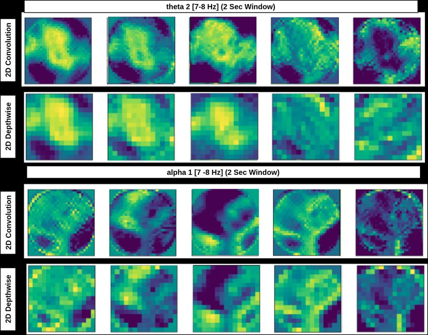
2       Pandey & Miyapuram

techniques. One of the complex problems was classification. In the short span of
4 years from 2012 to 2015, the ImageNet image-recognition challenge, which in-
cludes 1000 different classes in 1.2 million images, has consistently shown reduced
error rates from 26% to below 4% using CNN as the major component [21]. Iden-
tification of brain activity using CNNs has established remarkable performance
in several brain imaging datasets, including functional MRI, EEG, and MEG.
For example, Payan and Montana classified Alzheimer’s and healthy brains with
95% accuracy using 3D convolution layers on the ADNI public dataset contain-
ing 2265 MRI scans [25]. In the recent work, Dhananjay and colleagues imple-
mented three layers of CNN architecture to predict the song from EEG brain
responses with 84% accuracy, despite having several challenges such as having
low SNR, complex naturalistic music, and human perceptual differences [30].
However, all these models are building complex and deep networks without con-
sidering the limitation of time and resources. Two main concerns observed with
deep and wide architectures are having the millions of parameters that lead to
high computational cost and memory requirement. Therefore, this opens up the
opportunity to navigate the research to develop lightweight domain-specific ar-
chitectures for resource and time constraint environments. One such scenario is
a real-time analysis of EEG signals.
     EEG brain recordings have a high temporal resolution as well as a wide
variety of challenges such as low signal-to-noise ratio, noise can be of different
shape, for example, artifacts from eye movement, head movement, and electrical
line noise [20]. Hence, to extract significant features, it requires a sophisticated
and efficient method that considers the spatial information in depth. In recent
times, deep learning methods have been showing a significant improvement over
traditional machine learning algorithms. And, DL models have been expanding in
real-time computation also. Real-time analysis requires fast train as well as test
time. The major property that should hold in lightweight architecture is to design
the blocks, which reduces trainable parameters while maintaining state-of-the-
art performance [31]. A recent paper[30] on the classification of EEG signals has
introduced a significant performance by generating the time-frequency images
from EEG signals, but the proposed model is made of several components, which
loads the model with 5.8 million parameters. In this study, we have proposed a
novel pipeline to generate 2D images from EEG signals and develop a model that
produces comparable performance with state-of-the-art networks with minimum
time for training and testing and suitable for EEG classification tasks.

2     Related Studies
2.1   Cognitive Relevance
Meditation is a mental practice that enhances several cognitive abilities such
as enhancing attention, minimizing mind wandering, and developing sustained
attention [7]. EEG is the most widely used technique in the neuroscientific study
of meditation. EEG signals are decomposed into five frequency bands, including
delta (1-4Hz), theta (5-8 Hz), alpha (8-12 Hz), beta (13-30 Hz), and gamma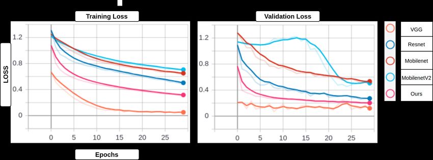
Brain2Depth:Lightweight CNN Model           3

Fig. 1. NeuroFeedback protocol: EEG signals are passed to the neural computational
toolbox, including preprocessing and analysis stages. Analysis pipeline comprises re-
quired computational algorithms, which generate feedback for the participant in real-
time with minimum lag.

(30-70 Hz). Several meditation studies report the importance of theta and alpha
waves for enhancing attention and are associated with several cognitive processes
[5]. These findings led the researchers to design a neurofeedback protocol [6] to
modulate oscillatory activities on the naive participants; a mechanism derives
from the focused-attention meditation technique. Neurofeedback is a process to
provide visual/audio feedback to a participant while recording his/her neural
responses in real-time, which develops skills to self-regulate electrical activity
of the brain, as shown in Fig.1. Previous studies on neurofeedback have shown
promising results to enhance performance, including athletes (archers improve
their shooting performance), musicians, professional dancers, and non-artists
to attain skills resembling visual artists [27]. NeuroFeedback requires a time-
efficient and high-performing computational technique in terms to classify the
different stages of brain responses.

2.2   Deep Learning Networks

There are four state-of-the-art architectures that have been the best way to
understand the significance of performance and light-weight architecture.
    Deep CNN Architectures: Deep CNNs (DCCN) have been introduced to
generate local low-level and mid-level feature learning in the initial layers and
high-level and global learning in the deeper layers. High-level features are the
combination of low and mid-level features. VGG is one of those DCNNs that
decreased the ImageNet error rate from 16% to 7% [29]. VGG expresses Visual
Geometry Group. They employed small convolution filters of size 3×3 in place
of the large filters comprising 11×11, 5×5 filters and observed the significant
performance with varying depth of the network. The use of small filters also
reduced the no of parameters, thus decreasing the number of computations.
ResNet50 is the next powerful and successful network after VGG, which stands
for residual networks having 50 layers [15]. ResNet was introduced to address
two problems. The network has the ability to bypass a layer if the present layer
could decrease performance and leads to overfitting, and this process is referred
to as identity mapping. Another significance is to allow an alternate shortcut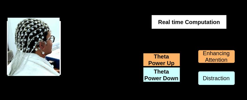
4      Pandey & Miyapuram

path for the gradient to flow that could avoid vanishing gradients problem [12].
ResNet decreased the error rate of 7%(VGG) to 3.6%.
    Lightweight CNN Architectures: MobileNet V1 was an early attempt to
introduce the lightweight model [16]. The remarkable performance of this model
was achieved by substituting the standard convolution operation with depthwise
separable convolution. This enhances the feature representation, which makes
the learning more efficient. The two primary components of depthwise separable
convolution are depthwise and pointwise convolution, which are introduced to
adjust channels and reduce parameters [18]. The stacking of these two compo-
nents generates novelty in the model. After this, another model proposed was
Mobilenet V2 [26]. Mobilenet V2 is the extension of Mobilenet V1. Sandler and
colleagues identified that non-linear mapping in lower-dimension increased infor-
mation loss. To address this problem, a significant module was introduced with
three consecutive operations. Initially, the dimension of feature maps is expanded
using 1×1 convolution, followed by, a depthwise convolution of 3×3 to retain the
abstract information. And in the last part, all the channels are condensed into
a definite size using 1×1 pointwise convolution. These transformations are pro-
cessed into a bottleneck residual block which is the core processing unit in place
of standard convolution.
    In our study, we use standard and depthwise convolution to enhance the per-
formance and depthwise separable convolution to make the model time-efficient.
The novelty of our work lies in the proposed pipeline to develop 2D plots from
EEG signals having 3 RGB channels representing power spectral, which pre-
serves the oscillatory information along with spatial position of electrodes. We
classify three cognitive states comprising expert, non-expert meditative states,
and control states (no prior experience of meditation). This paper discusses the
following components a) Our proposed pipeline b) Experimentation on Dataset
c) Comparative studies of ML and DL models d) Ablation Study

3     Data and Methods

3.1   Data and Preprocessing

We used two open-access repositories consisting of Himalayan yoga meditators
and controls [4,3]. In this research, we used EEG data of 24 meditators and 12
control subjects. Twenty-four meditators were further divided into two groups
comprising twelve experts and twelve non-experts. Data were captured using 64
channels Biosemi EEG system at the Meditation Research Institute (MRI) in
Rishikesh, India. Experimental design and complete description are mentioned
in the paper [5]. The expert group had an experience of a minimum of 2 hours
of daily meditation for one year or longer, whereas non-experts were irregu-
lar in their practice. Control subjects had no prior meditation experience and
were asked to pay attention to the breath’s sensations, including inhalation and
exhalation. A recent study [24] has shown the significant differences between ex-
pert and non-expert meditators and refers to as two distinct meditative states.
Brain2Depth:Lightweight CNN Model 5
Here, we refer to meditative and control states as cognitive states. As it in-
cludes cognitive components, such as involvement of attention during inhalation
and exhalation of breathing, practitioners engaging in mantra meditation which
enhances elements of sustained attention and language[5,22,2]. EEG data cor-
responding to breathing and meditation were extracted and preprocessed using
Matlab, and EEGLAB software [11]. We classified three states emerging from
expert, non-expert, and control groups, respectively.
EEG signals were downsampled at 256 Hz. A high pass linear FIR filter of
1 Hz was applied followed by removing the line noise artifacts at frequencies
of 50,100,150,200, 250. Artifact correction and removal were performed using
Artifact Subspace Reconstruction (ASR) method. Bad channels were removed
and spherical interpolation was performed for reconstructing the removed signal,
an essential step to retain the required signal. Data were re-referenced to aver-
age. Independent Components Analysis (ICA) was applied to classify the brain
components and to remove the artifacts, including eye blink, muscle movement,
signals generated from the heart, and other non-biological sources.
3.2 Methods
We divide the classification pipeline into two processing units. The first is to
create power spectral density 2D plots from neural responses, known as “Neural
Timeseries to 2D” and the second is to define the classification model term as
“2D to Prediction” as shown in Fig. 2.
1. Neural Timeseries to 2D: We divide the process of creating images from
EEG signals into the following three steps.
(a) Window Extraction: EEG time-series signals are extracted into windows
of 2, 4, and 6 seconds. For example, if a signal contains 24 seconds, we get
12, 6, and, 4 no of windows respectively. Varying window length identifies
the information content and plays a significant role in discriminating
the classes. In some applications, we have the luxury to extract varying
windows sizes depending on the task.
(b) Power Spectral Analysis: Power spectral density (PSD) is estimated for
the extracted window using the Welch method [13]. Welch’s method is
also known as the periodogram method for computing power spectrum,
the time signal is divided into successive blocks followed by creating a
periodogram for each block, and estimating the density by averaging.
Oscillatory cortical activity related to meditation primarily observes in
two frequency bands, theta (5-8Hz) and alpha (9-12Hz) [5]. These bands
are further subdivided into theta1(5-6Hz),theta2(7-8 Hz), and alpha1(9-
10Hz), alpha2(11-12Hz). For every channel, PSD is computed for the
mentioned four bands.
(c) Topographic (2D- 3 Channel) Plot: We use the topoplot function of the
EEGLAB that transforms the 3D projection of electrodes in a 2-D cir-
cular view using interpolation on a fine cartesian grid [14]. Topographic
plots were earlier implemented in Bashivan’s work [1], and they combined6 Pandey & Miyapuram
plots from three bands to form one image of three channels, whereas we
create one image of size 32 × 32 for each band having three RGB chan-
nels, and this might help to understand the significance of each band
in the specific cognitive task. This plot preserves the relative distance
between the neighboring electrodes and their underlying interaction, gen-
erating task-based latent representation using convolution.
(a)Neural TimeSeries Signals to 2D: Images are formed using power spectral analysis.
(b) 2D to Prediction: Images are fed into a deep learning network comprising of 4 blocks.
Fig. 2. Proposed pipeline for classification
2. 2D to Prediction: Our model comprises 4 Blocks as shown in Fig. 2 (b).
The first two blocks are introduced to capture deep feature information and
the third block for reducing the computation. The major components in
these three blocks are regular Conv2D, depthwise spatial Conv2D, depthwise
separable convolution, max pooling, ReLu(Rectified Linear Unit) activation
function, and batch normalization.Brain2Depth:Lightweight CNN Model 7
Conv2D to learn richer features at every spatial scale. Depthwise convolution
which acts on each input channel separately and extremely efficient to gen-
erate succinct representation [9]. Depthwise separable convolutions factorize
a regular convolution into a depthwise convolution and a (1,1) convolution
called a pointwise convolution [17]. This was initially introduced for generic
object classification [28] and later used in Inception models [19] to reduce
the computation in the first few layers. Kernel sizes for the initial two blocks
are 3×3 and 2×2 for standard 2D convolution with 64 filters and 2×2 for
Depthwise convolution. The third block comprises standard Conv2D and
depthwise separable convolution of kernel size 2×2 with 64 and 12 filters
respectively. ReLu activation is introduced in the initial two layers to pre-
pare the network to learn complex representations and to generate faster
convergence and better efficiency [23]. The output of ReLu is processed by
the Max Pooling operations for spatial sub-sampling, which downsample the
feature maps by generating features in patches of the feature map [9]. Batch
normalization is performed at last in the three blocks to minimize internal
covariate shift, which subsequently accelerates the training of deep neural
nets and enables higher learning rates [19].
Fourth block contains flatten, two dense layers and a softmax activation
function. A dense layer is employed to combine all the features learned from
previous layers where every input weight is directly connected to the output
of the next layer in a feed-forward fashion. Since we are doing multiclass
classification, the output layer has a softmax activation function. Softmax
as an activation function is used because the model requirement is to predict
only the specific class, which results in high probability. To find out the loss
of the model, categorical cross-entropy is used to predict the probability of
a class.
Deep learning models are trained using tensorflow(keras) [10] and machine
learning algorithms employ scikit learn library [8]. GPU NVIDIA GTX
1050(4GB RAM) are used for this study and the batch size are set to 30
because of memory constraints and kept the maximum epoch to 30 to main-
tain the timing constraint as well as to avoid overfitting and for optimal
training and validation loss.
4 Results and Discussion
This section discusses five measures a) performance of our model b) comparison
of time and parameters c) training and validation loss d)visualization of layers
e) ablation study
4.1 Performance
Baseline Methods: We compared the performance with commonly used classi-
fiers and state of the art deep learning models. We trained six machine learning
classifiers and tried several hyperparameters as shown in Table 1 and reported8 Pandey & Miyapuram
the maximum accuracy for all except NLSVM because it was around chance level.
We experimented with four state of the art deep learning models VGG16[29],
ResNet50[15], MobileNet[16], MobileNetv2[26] and keep block4 of our model as
the last block in all the models. These models are best suited for classification
tasks. We reported the cross-subject average accuracy using leave one out valida-
tion, eleven subjects from each condition were used for training and one subject
from each condition was used for testing and then reported the average accuracy
of 12 iterations. For example, in the 2-sec window, 9909 samples were used for
training and 1101 for validation and 813 samples for testing, this was iterated
for twelve times.
Table 1. Machine Learning Classifiers
Classifier Parameters
Linear SVM
penalty parameter C values: 0.1,0.5,1.5,5,20,40,80,120,150
(SVM)
Non Linear kernel: ’rbf’, upper bound on the fraction of margin errors
SVM (NLSVM) nu : 0.3,0.4,0.5, 0.6
algorithm = SAMME.R, no of estimators : 50, 100,200,250,
AdaBoost (AB)
300,400
Logistic
regularisation : l1, solver: saga
Regression (LR)
Linear
Discriminant threshold rank estimation = 0.0001
Analysis(LDA)
Random no of estimators: 50,100,150,200,250,300,400, min samples
Forest( RF) leaf:5, criterion: entropy
We obtained maximum accuracy 64.3% in theta1, 60.8% in theta2, 56.5% in
alpha1, and 56.1% in alpha2 for a 2-sec window using Random Forest Classifier
as shown in Fig. 3. Deep learning models completely outperformed traditional
ML techniques, we obtained 97.27% in VGG16, 91.01% in ResNet50, 90.75% in
MobileNet, 88.73% in MobilenetV2 and 94.57% in Brain2Depth(Ours) for theta1
in 2sec window as shown in Fig. 4. The minimum accuracy in traditional classi-
fiers might be due to utilizing the images directly for training by flattening the
images into a features matrix. There might be an improvement if we could have
tried with power spectral features but didn’t anticipate performance compara-
ble with DL models. This cannot preserve the spatial position as the topo plot
does. However, when compared our model with DL models showed comparable
performance in all windows.Brain2Depth:Lightweight CNN Model 9 Fig. 3. Performance of ML Models: Classification of three cognitive states; expert, non-expert meditative states, and control. Each box indicates five accuracy values representing classifiers mentioned in the right top corner. Bold text represents the maximum value in the box. Fig. 4. Performance of CNNs: Each column of a box represents accuracy, precision, recall, and f1-score, and row indicates the CNN network mentioned on the right top corner.
10 Pandey & Miyapuram
4.2 Parameters and Time
Parameters define the complexity of a model, we tried to keep our model simple
and explainable so that each block can be understood easily. We compared the
parameters and time for training and testing. Brain2Depth demonstrated com-
parable performance while using parameters which were only 0.52% of VGG16,
0.32% of ResNet50, 2.28% of MobileNet, and 3.16% of MobileNetV2. The train-
ing and testing time of our model for 9909 samples and 813 samples were 84.882
and 0.152 seconds whereas the mobilenet took the minimum time in all four
models, which were 214.989 and 0.44 seconds. Fast training may help to develop
a model fast with millions of images and make a quick deployment. Minimum
test time is most important in real-time prediction.
Table 2. The number of trainable parameters in each network with train and test
time, respectively.
Testing per
Model Parameters Training Time(s) Testing time(s)
sample(ms)
VGG16 14780739 652 0.473 0.582
ResNet50 23850371 847.483 1.119 1.376
MobileNet 3360451 214.989 0.44 0.541
MobileNetV2 2422339 258.503 0.702 0.863
Ours 76627 84.882 0.152 0.187
Table 3. Test performance of each iteration on theta1 band of 2-sec window: Training
performed on 33 subjects and testing on 3 subjects, including all conditions. Bold
values represents two best performance.
Model 1 2 3 4 5 6 7 8 9 10 11 12
VGG16 0.839 0.915 0.957 0.985 0.996 1 0.998 0.988 0.998 0.999 0.997 1
RESNET50 0.701 0.617 0.834 0.934 0.975 0.989 0.975 0.939 .989 .998 .988 0.99
Mobilenet 0.619 0.689 0.786 0.935 0.974 0.996 0.981 0.946 0.986 0.993 0.998 0.988
MobilenetV2 0.626 0.674 0.7 0.864 0.935 0.975 0.985 0.931 0.985 0.996 0.994 0.982
Ours 0.797 0.852 0.865 0.946 0.987 0.997 0.998 0.915 1 0.999 0.996 0.998
4.3 Training vs Performance Tradeoff
ResNet, MobileNet, and MobileNetV2 performed a little low when compared
with VGG and Brain2Depth for a 2-sec window in theta1 . We further explored
the subjectwise performance to understand the differences. We found that accu-
racy dropped significantly for one and two iterations as shown in the Table 3. In
the next step, we investigated training and validation loss to verify whether this
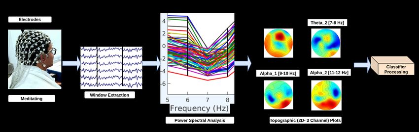
happened because of overfitting or underfitting. Fig. 5 shows that training lossBrain2Depth:Lightweight CNN Model 11 is high for three comparatively with others too. This shows that it may require more training rounds for this specific case however our model demonstrates that with moderate training it may perform well. And ResNet is a heavy architecture it may also require a large number of training samples. Hence with optimal time, our network can be trained efficiently even though the training sample can be noisy or varying samples. Fig. 5. Training and validation loss of the first iteration in theta1 band of 2-sec window with respect to all networks. Fig. 6. Visualization of Block1 Layers: Intermediate representation of standard and depthwise convolution layers in theta2 (7-8 Hz) and alpha1 (9-10 Hz) bands for expert meditators. 4.4 Visualization We have visualized the intermediate CNN outputs in block1 for two frequency bands i.e. theta2 and alpha1. Fig. 6 shows the outputs of five filters for 2D con-
12      Pandey & Miyapuram

volution and depthwise convolution in the expert condition. Layers have learned
the different features, more specifically in theta2, the frontal region has shown
the heightened contribution as compared with alpha1. This has also been studied
in meditation research on the role of the frontal midline region in the experienced
meditators [5].

Table 4. Ablation Study: Performance evaluation on 2-sec window with (A) several
changes in the number of filters and kernel sizes from block1 to block3. (B) change the
order of Relu, Batch Normalization, and Max pooling (C) modify layer with another
layer.

4.5   Ablation and Performance Studies
We provide detailed ablation and performance studies. We exploited our model
in the following three ways and reported the significant observations.
 1. Variation in Filters: Different level of granularity in the learning represen-
    tation depends on the size and number of filters. Small-size filters generate
    fine-grained information, whereas large-size filters represent coarse-grained
    information. We varied the number of filters and their sizes into three blocks
    as shown in Table 4 A. We kept the two blocks intact and changed the left
    block and observed the performance. No. of parameters ranged from 49K
    to 91K, and observed performance changes with varying parameters. Even
    with 53K parameters in block1, we found a significant performance above
    90% in all the bands. This shows that our presented model can be further
    customized according to the need.
 2. Swapping of components: We swapped the positions of batch normaliza-
    tion, Relu, and max-pooling. We didn’t observe any significant differences
    as shown in Table 4 B.
Brain2Depth:Lightweight CNN Model 13
3. Change in layers: In each block, we replaced one layer type with another layer
as shown in Table 4 C. We replaced depthwise convolution with standard
convolution. We observed a slight improvement by (1-2)% in all the frequency
bands however parameters got double and increased the training timing by
7 seconds. Hence, this suggests that the model can be efficiently fine-tuned
according to the availability of the resources and other constraints such as
time.
5 Conclusion
This study exhibits a pipeline for the EEG classification task, incorporating steps
to create topo images from EEG signals and a lightweight CNN model. In several
medical domains, heavy deep architectures are not required, and a simple model
is needed to produce similar results with less time. Our proposed study shows
state-of-the-art performance while using only 0.52% and 3.16% parameters of the
VGG and MobileNetV2 network, leading to a significant reduction in train and
test time. Our model can be efficiently deployed in several real time protocols
and effectively suited for resource constraint environment.
6 Acknowledgement
We thank SERB and PlayPower Labs for supporting PMRF Fellowship. We
thank FICCI to facilitate this PMRF Fellowship. We thank Kushpal, Pragati
Gupta and Nashra Ahmad for their valuable feedback.
References
1. Bashivan, P., Rish, I., Yeasin, M., Codella, N.: Learning representations
from eeg with deep recurrent-convolutional neural networks. arXiv preprint
arXiv:1511.06448 (2015)
2. Basso, J.C., McHale, A., Ende, V., Oberlin, D.J., Suzuki, W.A.: Brief, daily
meditation enhances attention, memory, mood, and emotional regulation in non-
experienced meditators. Behavioural brain research 356, 208–220 (2019)
3. Braboszcz, C., Cahn, B.R., Levy, J., Fernandez, M., Delorme, A.: Increased gamma
brainwave amplitude compared to control in three different meditation traditions.
PLoS One 12(1), e0170647 (2017)
4. Brandmeyer: Bids-standard: bids-standard/bids-examples, https://github.com/
bids-standard/bids-examples/tree/master/eeg_rishikesh
5. Brandmeyer, T., Delorme, A.: Reduced mind wandering in experienced medita-
tors and associated eeg correlates. Experimental brain research 236(9), 2519–2528
(2018)
6. Brandmeyer, T., Delorme, A.: Closed-loop frontal midlineθ neurofeedback: A novel
approach for training focused-attention meditation. Frontiers in Human Neuro-
science 14, 246 (2020)14 Pandey & Miyapuram
7. Brandmeyer, T., Delorme, A., Wahbeh, H.: The neuroscience of meditation: classifi-
cation, phenomenology, correlates, and mechanisms. In: Progress in brain research,
vol. 244, pp. 1–29. Elsevier (2019)
8. Buitinck, L., Louppe, G., Blondel, M., Pedregosa, F., Mueller, A., Grisel, O., Nic-
ulae, V., Prettenhofer, P., Gramfort, A., Grobler, J., Layton, R., VanderPlas, J.,
Joly, A., Holt, B., Varoquaux, G.: API design for machine learning software: expe-
riences from the scikit-learn project. In: ECML PKDD Workshop: Languages for
Data Mining and Machine Learning. pp. 108–122 (2013)
9. Chollet, F.: Xception: Deep learning with depthwise separable convolutions. In:
Proceedings of the IEEE conference on computer vision and pattern recognition.
pp. 1251–1258 (2017)
10. Chollet, F., et al.: Keras (2015), https://github.com/fchollet/keras
11. Delorme, A., Makeig, S.: Eeglab: an open source toolbox for analysis of single-trial
eeg dynamics including independent component analysis. Journal of neuroscience
methods 134(1), 9–21 (2004)
12. Dhillon, A., Verma, G.K.: Convolutional neural network: a review of models,
methodologies and applications to object detection. Progress in Artificial Intel-
ligence 9(2), 85–112 (2020)
13. EEGLAB: Sccn: sccn/eeglab, https://github.com/sccn/eeglab/blob/develop/
functions/sigpro\cfunc/spectopo.m
14. EEGLAB: Sccn: sccn/eeglab, https://sccn.ucsd.edu/~arno/eeglab/auto/
topoplot.html
15. He, K., Zhang, X., Ren, S., Sun, J.: Deep residual learning for image recognition. In:
Proceedings of the IEEE conference on computer vision and pattern recognition.
pp. 770–778 (2016)
16. Howard, A.G., Zhu, M., Chen, B., Kalenichenko, D., Wang, W., Weyand, T., An-
dreetto, M., Adam, H.: Mobilenets: Efficient convolutional neural networks for
mobile vision applications. arXiv preprint arXiv:1704.04861 (2017)
17. Howard, A.G., Zhu, M., Chen, B., Kalenichenko, D., Wang, W., Weyand, T., An-
dreetto, M., Adam, H.: Mobilenets: Efficient convolutional neural networks for
mobile vision applications. arXiv preprint arXiv:1704.04861 (2017)
18. Hua, B.S., Tran, M.K., Yeung, S.K.: Pointwise convolutional neural networks. In:
Proceedings of the IEEE Conference on Computer Vision and Pattern Recognition.
pp. 984–993 (2018)
19. Ioffe, S., Szegedy, C.: Batch normalization: Accelerating deep network training by
reducing internal covariate shift. arXiv preprint arXiv:1502.03167 (2015)
20. Jiang, X., Bian, G.B., Tian, Z.: Removal of artifacts from eeg signals: a review.
Sensors 19(5), 987 (2019)
21. Khan, A., Sohail, A., Zahoora, U., Qureshi, A.S.: A survey of the recent architec-
tures of deep convolutional neural networks. Artificial Intelligence Review 53(8),
5455–5516 (2020)
22. Lee, D.J., Kulubya, E., Goldin, P., Goodarzi, A., Girgis, F.: Review of the neural
oscillations underlying meditation. Frontiers in neuroscience 12, 178 (2018)
23. Nair, V., Hinton, G.E.: Rectified linear units improve restricted boltzmann ma-
chines. In: ICML (2010)
24. Pandey, P., Miyapuram, K.P.: Classifying oscillatory signatures of expert vs non-
expert meditators. In: 2020 International Joint Conference on Neural Networks
(IJCNN). pp. 1–7. IEEE (2020)
25. Payan, A., Montana, G.: Predicting alzheimer’s disease: a neuroimaging study with
3d convolutional neural networks. arXiv preprint arXiv:1502.02506 (2015)Brain2Depth:Lightweight CNN Model 15
26. Sandler, M., Howard, A., Zhu, M., Zhmoginov, A., Chen, L.C.: Mobilenetv2: In-
verted residuals and linear bottlenecks. In: Proceedings of the IEEE conference on
computer vision and pattern recognition. pp. 4510–4520 (2018)
27. Sho’ouri, N., Firoozabadi, M., Badie, K.: The effect of beta/alpha neurofeedback
training on imitating brain activity patterns in visual artists. Biomedical Signal
Processing and Control 56, 101661 (2020)
28. Sifre, L., Mallat, S.: Rigid-motion scattering for image classification. Ph. D. thesis
(2014)
29. Simonyan, K., Zisserman, A.: Very deep convolutional networks for large-scale
image recognition. arXiv preprint arXiv:1409.1556 (2014)
30. Sonawane, D., Miyapuram, K.P., Rs, B., Lomas, D.J.: Guessthemusic: song iden-
tification from electroencephalography response. In: 8th ACM IKDD CODS and
26th COMAD, pp. 154–162 (2021)
31. Wu, J., Tang, T., Chen, M., Wang, Y., Wang, K.: A study on adaptation lightweight
architecture based deep learning models for bearing fault diagnosis under varying
working conditions. Expert Systems with Applications 160, 113710 (2020)
32. Zhang, Q., Zhang, M., Chen, T., Sun, Z., Ma, Y., Yu, B.: Recent advances in
convolutional neural network acceleration. Neurocomputing 323, 37–51 (2019)You can also read