Bone Stress-Strain State Evaluation Using CT Based FEM
←
→
Page content transcription
If your browser does not render page correctly, please read the page content below
ORIGINAL RESEARCH
                                                                                                                                             published: 18 June 2021
                                                                                                                                    doi: 10.3389/fmech.2021.688474

                                           Bone Stress-Strain State Evaluation
                                           Using CT Based FEM
                                           Oleg V. Gerasimov 1, Nikita V. Kharin 1, Artur O. Fedyanin 2, Pavel V. Bolshakov 1,
                                           Maxim E. Baltin 2, Evgeny O. Statsenko 3, Filip O. Fadeev 4, Rustem R. Islamov 4,
                                           Tatyana V. Baltina 2 and Oskar A. Sachenkov 1*
                                           1
                                            Department of Theoretical Mechanics, Institute of Mathematics and Mechanics, Kazan Federal University, Kazan, Russia,
                                           2
                                            Department of Human and Animal Physiology, Institute of Fundamental Medicine and Biology, Kazan Federal University, Kazan,
                                           Russia, 3Laboratory of X-ray Tomography, Institute of Geology and Petroleum Technologies, Kazan Federal University, Kazan,
                                           Russia, 4Department of Medical Biology and Genetics, Kazan State Medical University, Kazan, Russia

                                           Nowadays, the use of a digital prototype in numerical modeling is one of the main
                                           approaches to calculating the elements of an inhomogeneous structure under the
                                           influence of external forces. The article considers a finite element analysis method
                                           based on computed tomography data. The calculations used a three-dimensional
                                           isoparametric finite element of a continuous medium developed by the authors with a
                                           linear approximation, based on weighted integration of the local stiffness matrix. The
                                           purpose of this study is to describe a general algorithm for constructing a numerical model
                          Edited by:       that allows static calculation of objects with a porous structure according to its computed
        Mohammad Hossein Heydari,          tomography data. Numerical modeling was carried out using kinematic boundary
 Shiraz University of Technology, Iran
                                           conditions. To evaluate the results obtained, computational and postprocessor grids
                       Reviewed by:
                          Jianing Wu,      were introduced. The qualitative assessment of the modeling data was based on the
      Sun Yat-Sen University, China        normalized error. Three-point bending of bone specimens of the pig forelimbs was
                Amir Putra Md Saad,
 Universiti Teknologi Malaysia (UTM),
                                           considered as a model problem. The numerical simulation results were compared with
                             Malaysia      the data obtained from a physical experiment. The relative error ranged from 3 to 15%, and
                 *Correspondence:          the crack location, determined by the physical experiment, corresponded to the area
                 Oskar A. Sachenkov        where the ultimate strength values were exceeded, determined by numerical modeling.
                       4works@bk.ru
                                           The results obtained reflect not only the effectiveness of the proposed approach, but also
                    Specialty section:     the agreement with experimental data. This method turned out to be relatively non-
         This article was submitted to     resource-intensive and time-efficient.
          Biomechanical Engineering,
               a section of the journal    Keywords: bone imaging, bone health, fracture risk, FEM, CT, CT/FEA
  Frontiers in Mechanical Engineering
            Received: 09 April 2021
           Accepted: 07 June 2021          INTRODUCTION
           Published: 18 June 2021
                              Citation:    At the moment, numerical modeling is the main calculation method in various fields of scientific
             Gerasimov OV, Kharin NV,      research. And the use of data from experimental samples’ images is the most promising approach to
          Fedyanin AO, Bolshakov PV,       describing the behavior of elements of inhomogeneous structures under external the influence
Baltin ME, Statsenko EO, Fadeev FO,        (Mithun and Mohammad, 2014; Marwa et al., 2018). This approach allows us to consider problems
            Islamov RR, Baltina TV and
                                           with multi-connected porous or inhomogeneous materials (Kayumov, 1999; Alberich-Bayarri et al.,
 Sachenkov OA (2021) Bone Stress-
      Strain State Evaluation Using CT
                                           2008; Kharin et al., 2019). This is especially true in clinical practice since it can significantly affect the
                           Based FEM.      quality of treatment (Kichenko et al., 2008; Kichenko et al., 2011; Maquer et al., 2015). Stress-strain
          Front. Mech. Eng 7:688474.       state is important in tasks to estimate bone remodeling, especially in the case of patient-based
    doi: 10.3389/fmech.2021.688474         implant design (Maslov, 2017; Borovkov et al., 2018; Maslov, 2020). There are several image-based

Frontiers in Mechanical Engineering | www.frontiersin.org                         1                                            June 2021 | Volume 7 | Article 688474
Gerasimov et al.                                                                                                                     CT Based FEM Application

approaches to determining the mechanical parameters of the                  MATERIALS AND METHODS
model. One of them is based on approximating the
inhomogeneity by constructing a distribution using the mean                 Computed Tomography Based Finite
intercept length method. With this approach, the physical                   Element
relations are expressed in terms of the tensor of elastic                   Let’s consider the region describing the volume of an object.
constants and the fabric tensor (Sachenkov et al., 2016;                    Additionally, there is digital data of the object. In the research
Kayumov et al., 2018; Yaikova et al., 2019). The next                       computed tomography data is understood as a digital
approach is based on reducing the material anisotropy to                    prototype. The data consists of a number of microvolumes
orthotropy by calculating constants from numerical                          with an average value of the Hounsfield unit. Usually, such data
experiments (Ruess et al., 2012; Ridwan-Pramana et al.,                     illustrated by a greyscale three-dimensional image. Each
2017; Chikova et al., 2018). Finally, the work presents a                   microvolumes (voxel) has dimensions Δx, Δy, Δz. Usually, a
third approach based on taking into account the material                    voxel is equal to a cube and the size depends on computed
properties by weighted integration of the global stiffness                  tomography resolution. The mechanical behavior of the object
matrix of the finite element mesh.                                           will be investigated by the finite element methods. In this case,
    Computed tomography is the main approach to                             the volume is consists of a number of finite element. To
reconstructing images of the investigated domain. Such a                    simulate the inhomogeneity continuum three-dimensional
process implies the creation of its digital prototype, which is a           eight-node finite element with bilinear interpolation was
three-dimensional array of numbers corresponding to the                     built. Using shape functions Nn in the local coordinate
material permeability in each microelement (voxel) of the                   system of the element (ξn, ηn, ζn) the displacement can be
volume. These values can be interpreted according to                        presented as follows:
Hounsfield’s quantitative scale of X-ray density. Modern                                     ⎪
                                                                                            ⎧   ⎪       ⎪     ⎪
                                                                                            ⎨u⎫ ⎬     8 ⎧
                                                                                                        ⎨ un ⎫⎬
computed tomography (CT) allows getting detailed                                      {ϑ}  ⎪ v ⎪  ⎪ vn ⎪Nn ξ n , ηn , ζ n             (2.1.1)
information not only about bone tissue state but also its                                   ⎩ ⎭ i1 ⎩ ⎭
                                                                                              w            wn
interaction with implants (Stock et al., 2002; Jones et al., 2007;
Vanlenthe et al., 2007). Using CT data the segmentation can                 where u, v, w are components of a displacement vector in
be performed. It’s a complicated process because it’s important to          global coordinate system x, y, z, and shape function looks like
restore not only geometry but also the inner structure of the organ         N n(ξ, η, ζ)  (1 + ξ · ξn ) (1 + η·ηn ) (1 + ζ·ζn)/8.
(Supplementary Material). Wherein restored geometry should                     The equations can be presented in matrix from:
be meshed for simulation. The quality of mesh influences a lot on
                                                                                                          {ϑ}  [N] ϑE                               (2.1.2)
simulation quality. A common approach is to use stratified
segmentation. E.g., separate geometry for cortical and                      where {ϑE}—vector of the node displacements, [N]—matrix of the
cancellous bone tissue in whole bone (Marcián et al., 2018;                 shape functions.
Carniel et al., 2019). Then, in simulation, each geometry can                  Let’s introduce strain and stress vectors:
be taken into account with different mechanical properties
(Marcian et al., 2017; Hettich et al., 2018; Kuchumov and                                    {ε}  εxx , εyy , εzz , εxy , εyz , εzx               (2.1.3)
Selyaninov, 2020). But these actions are laborious and modern
                                                                                             {σ}  σ xx , σ yy , σ zz , σ xy , σ yz , σ zx         (2.1.4)
research focused on ways to facilitate the segmentation (Moriya
et al., 2018). On other hand, the highest calculation accuracy is              Using strain-displacement equations strain vector can be
achieved by modeling each microvolume of a continuous                       determined (Zienkiewicz and Zhu, 1987):
medium with one finite element (Prez et al., 2014; Tveito
et al., 2017). However, in this case, the computational intensity                                    {ε}  L ξ, η, ζ {ϑ}                           (2.1.5)
increases excessively. In this regard, it makes sense to increase the
                                                                            where [L]—differentiation matrix.
finite element size so that it contains a certain amount of
                                                                              Using Hooke’s law stress vector can be found:
microvolumes (Nadal et al., 2013; Marco et al., 2015;
Giovannelli et al., 2017). In this case, each voxel can be                                             {σ}  [D({r})]{ε}                             (2.1.6)
considered as a neighborhood of the integration point of the
local stiffness matrix. However, the question of the number of              where [D]—elasticity matrix, {r}—vector in a point where
voxels in the element volume is still open. The same question is            elasticity matrix set.
open for applicability of finite element method (FEM) in casual                 In case of inhomogeneous media elasticity matrix can be
clinic practice (Viceconti et al., 2018).                                   rewritten in form:
    The purpose of the study is to implement the method of static                                [D({r})]  DB  · ω({r})                           (2.1.7)
calculation of problems based on samples of a porous structure. A
three-dimensional isoparametric linear element of a continuous              where [DB]—elasticity matrix of pure material, ω{r}—scalar
medium, built on the basis of computed tomography data, was                 function which determines inhomogeneity by digital
used as a finite element of the grid.                                        prototype data.

Frontiers in Mechanical Engineering | www.frontiersin.org               2                                              June 2021 | Volume 7 | Article 688474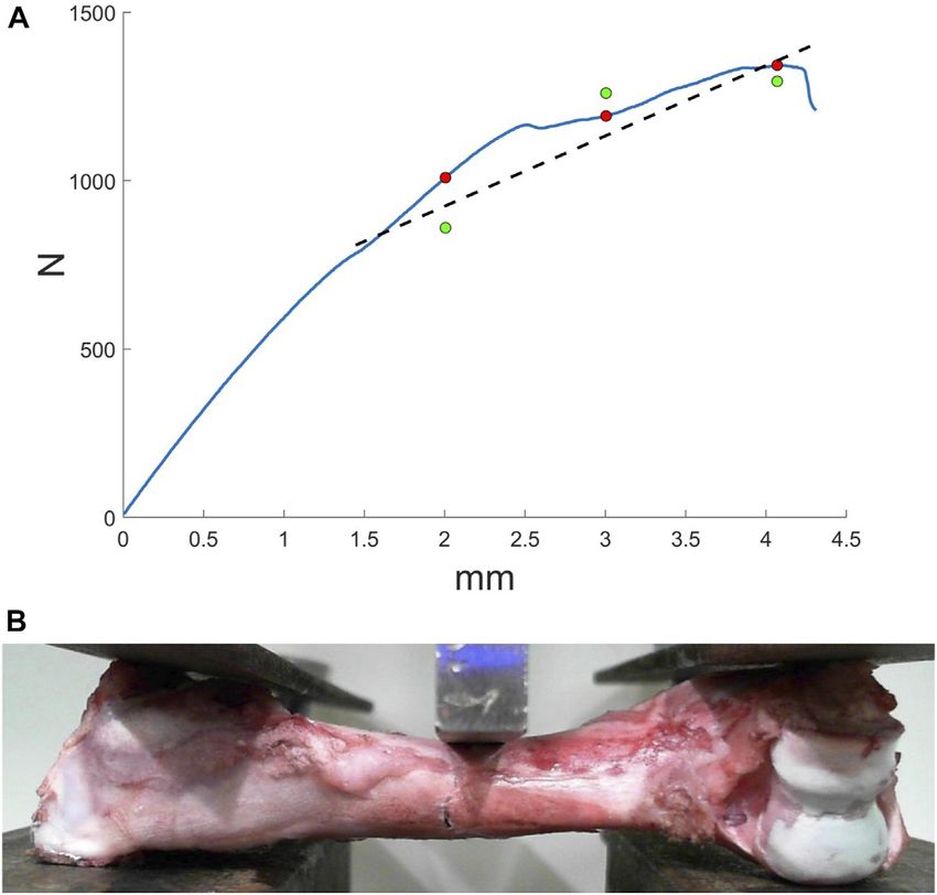
Gerasimov et al.                                                                                                              CT Based FEM Application

    The ω{r} function can be calculated using Hounsfield unit               Meshing and Segmentation
(HU) from CT data. And then strain vector can be rewritten as              Consider the global algorithm of the analysis of the bone. Input
follow:                                                                    data is presented as CT, where each value of HU can be
                                                                           interpreted as optical density and even can be recalculated to
                      {ε}  B ξ, η, ζ  · ω({r}) · {ϑ}      (2.1.8)
                                                                           elastic constants, and ultimate stress using equations (Rho et al.,
where matrix [B] is equal to [D ]·[L(ξ, η, ζ)].
                                          B                                1995):
  So stiffness matrix for an element can be denoted (Zienkiewicz                                    ρ  aρ + bρ · HU                            (2.2.1)
and Zhu, 1987):
                                                                                                   E  aE ρbE
                                                                                                                                                (2.2.2)
                                           T
           K E   ∭ 1−1 B ξ, η, ζ  [D]B ξ, η, ζ                                            [σ]  aσ ρ   bσ
                                                                                                                                                (2.2.3)

                        ξ, η, ζ ω ξ, η, ζ dξdηdζ
                    × J                                     (2.1.9)
                                                                           where coefficients a and b with the corresponding indices are
where |J(ξ, η, ζ)| is the Jacobian determinant of coordinate               determined from experiments or literature and can vary
transformation.                                                            depending on the type of bone tissue or organ.
   When node displacements are found using differentiation                    Bone is a heterogeneous porous material with an irregular
matrix and elasticity matrix strain and stress vectors can be              structure. The process of constructing a finite element mesh over
found. Using shape functions for every element stress function             the selected area implies segmentation of the initial CT data. In
can be approximated:                                                       this case, each finite element is associated with a certain area of
                                                                           the bone. Such subregions are characterized by a different
        σ E ξ, η, ζ  ∭V E {N}T σ E0  − σ i dV → min      (2.1.10)       distribution of bone substance, which can include both the
                                                                           cortical plate and the spongy substance. Thus, the proposed
where σi—node value of stress, {σE0}—vector if approximation               method for constructing the finite element mesh makes it
coefficients.                                                               possible to take into account the material anisotropy at the
   So average stress in each element can be found:                         level of modeling an individual finite element based on its CT
                        σ E  VE−1 ∭V E {N}T σ E0 dV      (2.1.11)       data. Figure 1 sequentially shows subvolumes with different
                                                                           levels of porosity. On the left side is the area with a highest
where VE—element’s volume.                                                 porosity (cancellous zone), on the right one is the part
   To estimate computational error the energy norm should be               corresponding to a cortical plate. A popular approach is to use
calculated. For this purpose at every element stress error should          segmentation to restore the geometry of an organ. But researchers
be calculated:                                                             face difficulty when investigating organs with irregular geometry
                                                                           and complicated inner structure, e.g., femur, where there are
                            Δσ in   σ an  − σ in     (2.1.12)       cortical and cancellous regions. The proposed method allows
where {σan}—average stress vector at node n, {σin}—stress vector of        taking into account such anisotropy properties indirectly. Based
node n of finite element i.                                                 on the developed FE it is offered to use regular mesh for the whole
    Then, for each element, the energy error is calculated as              CT space. Using a threshold filter for porosity the mesh can be
follows (Grassi et al., 2012; Giovannelli et al., 2017):                   clarified. Let’s call such a mesh computational grid. Then
                                                                           kinematic or/and static boundary conditions can be applied.
                1
             E  ∭V E {Δσ}T [D]−1 ω−1 {Δσ}dV E                             Then all local stiffness matrixes can be calculated using CT
              i
                                                            (2.1.13)
                2                                                          data. Assembling the global stiffness matrix is a casual task.
   Strain energy of the element can be calculated by equation:             After nodal displacements are found average stress and strain
                                                                           vector for each element can be found. Principal values, directions,
                           i 1                                             and von Mises yield was calculated for average stress and strain in
                          U  ∭V E {σ}T {ε}dV E             (2.1.14)
                             2                                             each element. To juxtapose stress-strain state and CT data
   Finally, the energy error can be normalized according to the            additional mesh was build. Let’s call such a mesh post-
strain energy:                                                             processing grid. Such a grid can be built as a contour of
                                                                   binarized CT data. So, results from the computational grid can
                                 E
                                   i                                       be interpolated to the post-processing grid.
                      ~ i
                      E       i     i ·100%           (2.1.15)               General algorithm
                             U +E
    So, the described approach allows taking into account the                 Input: CT data, boundary conditions
inhomogeneity of media in terms of the stiffness matrix. Analyses             Output: Post processing grid, nodal and element solutions
of stress-strain state should be held in terms of average stress and          1: generate regular mesh for hole CT space with given
strain. The quality of results can be judged by normalized energy             element size
error value. A more detailed description of the method and                    2: for each element in regular mesh
evaluation of element convergence depending on voxel                          3: if bone tissue relative content < bone threshold
number is given in the previous publications (Gerasimov et al.,               4: then delete element
2019; Gerasimov et al., 2021).                                                4: else compute local stiffness matrix according to CT data

Frontiers in Mechanical Engineering | www.frontiersin.org              3                                           June 2021 | Volume 7 | Article 688474
Gerasimov et al. CT Based FEM Application
FIGURE 1 | Three-dimensional visualization of CT data corresponding to different areas of the bone: porosity decreases from left to right, which, accordingly, leads
to an increase in the bone volume fraction.
4: End for reconstruction software was used. The sample fixed in the holder was
5: Save mesh as a computational grid placed on the rotating table of the X-ray computed tomography
6: Assembling the global stiffness matrix, apply boundary chamber at the optimum distance from the X-ray source. The survey
conditions and solve was carried out at an accelerating voltage of 90–100 kV and a current
7: Calculate stress and strain in elements 140–150 mA. After that three-point bending tests were carried out.
8: Generate post-processing grid using given HU threshold CT data was about 800–900 Mb, voxel size in the direction of
with given tolerance three Cartesian coordinate axes was equal to 0.2 mm. The data
9: Interpolate solution to post-processing grid dimension was equal to 7523. Based on CT data, an initial regular
finite element mesh was constructed. The computational grid
FEM software was implemented using C++ (g++ compiler). generation was based on the removal of elements with a bone
An Eight-node finite element with three degrees of freedom in substance content of less than 5%. In this case, the initial CT data
each node was realized. The algorithm was parallelized using was pre-binarized according to the specified threshold value:
OpenMP technology because of the high labor costs of integrating values less than the threshold value were equated to zero,
the local stiffness matrix. The solution of problems was carried out larger or equal—to one. Determination of the mechanical
on a computer with the following configuration: CPU—AMD Ryzen properties of bone tissue was based on the use of a similar
7 1700 with 8 physical and 16 logical cores with a frequency of binarization function. Young’s modulus for pure bone tissue
3.7 GHz, RAM—G. Skill Aegis 16 GB DDR4 3000 16GISB K2 C16 can be calculated by Eq. 2.2.2 and was equal to 30 GPa and
with a frequency of 2933 MHz, motherboard—MSI B350M Poisson’s ratio equal to 0.3. In calculations three-point bending
MORTAR. Post-processing was carried out using the ParaView simulation. The top and the bottom surfaces of the distal and the
software (Ahrens et al., 2005; Ayachit, 2015). proximal regions were fixed (marked by black lines in Figures
2A,C). Displacements in y negative direction were applied on the
Bending Test top surface of the medial region (marked by red arrows in Figures
Experiments were performed on six 15–20 kg male Vietnamese 2A,C) and were equal to 2, 3, and 4 mm, respectively. To verify
swine. Animals were placed in individual cages under standard the simulation results equivalent force was calculated. All steps of
laboratory conditions with unlimited access to food and water calculations from reading CT data to interpolate nodal and
and a 12 h day/night cycle. The protocol of the experiment, element solution to the post-processing grid took about 15 min.
including anesthesia, surgery, postoperative care, testing, and
euthanasia, was approved by the Animal Care Committee of
Kazan State Medical University (protocol #5 of 20 May 2020). All RESULTS AND DISCUSSION
experimental procedures were performed in accordance with the
standards to minimize animal suffering and the size of Two initial meshes with 10 and 5 mm element sizes were used.
experimental groups. Animals were included in experiments Normalized errors were analyzed for each result. Special attention
after a period of adaptation of at least 7 days. In experiments was paid to the value of normalized errors in elements where
bones of animals after contusion spinal injury were used. The maximum Von Mises stress appears. In Figure 2 distribution of
animals were sacrificed on the 8th week after a spinal cord injury normalized error (on computational grid) and Von Mises stress
(SCI). The euthanasia was performed under deep anesthesia by (on post processing grid) in forelimb is shown. It’s important to
overdosing on an inhalational narcosis agent (Isoflurane) (Fadeev understand correctly the meaning of the Von Mises stress in
et al., 2020). The bones of the fore and hind limbs were extracted. results. Averaging in element according to corresponding CT data
Bones were scanned by CT. Micro/nanofocal X-ray inspection change the understanding of the received value. In this case, we
system for CT and 2D inspections of Phoenix V | tome | X S240 was consider the element as a subvolume of the digital prototype with
used for scanning. The system is equipped with two X-ray tubes: unknown stress spatial distribution but a known mean value. It
microfocus with a maximum accelerating voltage of 240 kV power of means that falsely high and falsely low values can appear, that’s
320 W and nanofocus with a maximum accelerating voltage of 180 kV why normalized errors should be checked in the element. For
power of 15 W. For primary data processing and creating a volume both meshes maximum of normalized error appears in border
(voxel) model of the sample based on x-ray images, the datos|x elements where relative bone tissue content is low. It can be
Frontiers in Mechanical Engineering | www.frontiersin.org 4 June 2021 | Volume 7 | Article 688474Gerasimov et al. CT Based FEM Application FIGURE 2 | Distribution of normalized error and Von Mises stress: (A) normalized error for 10 mm mesh, (B) Von Mises stress for 10 mm mesh, (C) normalized error for 5 mm mesh, (D) Von Mises stress for 5 mm mesh. In (A,C) fixed regions marked by black lines and region where displacements were applied marked by red arrows. FIGURE 3 | Distribution of principal stresses and directions: (A), (B) 1st principal stress and direction, (C,D) 2nd principal stress and direction, (E,F) 3rd principal stress and direction. Frontiers in Mechanical Engineering | www.frontiersin.org 5 June 2021 | Volume 7 | Article 688474
Gerasimov et al.                                                                                                                              CT Based FEM Application

 FIGURE 4 | Results of three-point bending experiments: (A) force-displacement curve, where green markers indicate the equivalent force from the simulation, red
 markers correspond to the force form the experiment, dashed line—approximation of the equivalent force: (B) bone fracture formation.

explained by the stiffness matrix decrease in stiffness. It’s                          applied force in the same displacements (red markers in
important to notice that values of normalized error in regions                         Figure 4A). The relative error was from 3 to 15%. The region
of interest are below 50%. The maximum value of 50% is reached                         a crack appears in experiments matches the region in simulation.
in the location of kinematics boundary conditions are applied. In                      Of course, there were some deviations, which can be explained by
other regions, the normalized error is below 25%.                                      not accurate boundary conditions.
    Let’s focus on the task with 4 mm displacement applied and                             Despite the simple function for mechanical properties
consider the mesh with a 5 mm element size. The minimum of                             (binarization by threshold), adequate results were achieved. It can
normalized error (20%) and maximum of Von Mises (500 MPa)                              be explained by the stiffness matrix integration way. It proposes a
stress was in the region near applied loading (see Figures 2C,D).                      method to consider the bone tissue structure. In this case, nodal
For more detailed analyses principal stresses and directions were                      displacement in element conditioned not only by mechanical
found, which are shown in Figure 3. To estimate equivalent force                       properties but by material distribution. Previously it was shown
in displacements’ applied region 2nd principal stresses were used                      that bone volume fraction and material distribution influence much
(see Figures 3C,D). The integral of the stress vector in the region                    greater on mechanical properties than other morphological variables
multiplied by the area will consider as a reaction to equivalent                       (Maquer et al., 2015). To estimate the distribution approximation by
force. 1st and 3 days principal stresses describe the stress state of                  tensor is popular. But in practice, it means that at the first step such
the bone (see Figures 3A,B,E,F). Corresponding streamlines form                        tensor should be calculated, and then the tensors should be taken
an orthogonal system. It should be noticed that in the region of                       into account in mechanical model and simulation. The described
Von Mises maximum first principal stresses reach a maximum                              method allows taking into account structural properties indirectly by
value 400 MPa and 3 days principal—minimum −400 MPa. It                                stiffness matrix integration way. Add it costs less laborious.
explains the crack that appears in an experiment, cause the                                More than that, the proposed method allows using part of the
values exceed yield strength (Crenshaw et al., 1981; Imai, 2015).                      CT data space. In this case, the corresponding dimensions of the
    To verify simulation results equivalent force was compared                         initial mesh should be set. From a practical point of view after the
with force from three-point bending experiments. In Figure 4A                          region of interest is chosen boundary conditions should be applied.
force-displacement curve is shown. On curve marked values of                           So bone can be checked for strength. Typical loading cases can be
equivalent force (green markers in Figure 4A) and values of                            simulated. The quality of the solution can be estimated by

Frontiers in Mechanical Engineering | www.frontiersin.org                          6                                              June 2021 | Volume 7 | Article 688474
Gerasimov et al. CT Based FEM Application
normalized error. And analyses can be automated in terms of the AUTHOR CONTRIBUTIONS
normalized error and the stress invariants, e.g., Von Mises stress.
OG, NK, PB, TB, and OS design method, realized it on
programming language and wrote the manuscript. AF, MB,
CONCLUSION OS, FF, RI, ES, and TB conducted experimental data for
numerical calculation and contributed to manuscript writing.
The CT-based FEM method is introduced. A three-dimensional All authors have read and agreed to the published version of the
isoparametric linear element of a continuous medium, built on manuscript.
the basis of computed tomography data, presented. The general
algorithm to get the FE model is presented. For this purpose
computational and post-processing grids were introduced. To FUNDING
estimate the quality of simulation normalized error was used.
Three-point bending was simulated by the method and results This work was supported by the Russian Science Foundation
were compared with provided experiments. Received results (RSF grant No. 18-75-10027).
illustrate the effectiveness of the method.
ACKNOWLEDGMENTS
DATA AVAILABILITY STATEMENT
Special thanks to Interdisciplinary center for analytical
The raw data supporting the conclusion of this article will be microscopy of Kazan Federal University.
made available by the authors, without undue reservation.
SUPPLEMENTARY MATERIAL
ETHICS STATEMENT
The Supplementary Material for this article can be found online at:
The animal study was reviewed and approved by the Animal Care https://www.frontiersin.org/articles/10.3389/fmech.2021.688474/
Committee of Kazan State Medical University. full#supplementary-material
Gerasimov, O. V., Berezhnoi, D. V., Bolshakov, P. V., Statsenko, E. O., and
REFERENCES Sachenkov, O. A. (2019). Mechanical Model of a Heterogeneous Continuum
Based on Numerical-Digital Algorithm Processing Computer Tomography
Ahrens, J., Geveci, B., and Law, C. (2005). ParaView: An End-User Tool for Large Data. Russ. J. Biomech. 23 (1), 87–97.
Data Visualization, Visualization Handbook. Elsevier. ISBN-13: 978- Giovannelli, L., Ródenas, J. J., Navarro-Jiménez, J. M., and Tur, M. (2017). Direct
0123875822. Medical Image-Based Finite Element Modelling for Patient-specific Simulation
Alberich-Bayarri, A., Marti-Bonmati, L., Sanz-Requena, R., Belloch, E., and of Future Implantsfic Simulation of Future Implants. Finite Elem. Anal. Des.
Moratal, D. (2008). In Vivo Trabecular Bone Morphologic and Mechanical 136, 37–57. doi:10.1016/j.finel.2017.07.010
Relationship Using High-Resolution 3-T MRI. Am. J. Roentgenology 191 (3), Grassi, L., Schileo, E., Taddei, F., Zani, L., Juszczyk, M., Cristofolini, L., et al. (2012).
721–726. doi:10.2214/AJR.07.3528 Accuracy of Finite Element Predictions in Sideways Load Configurations for the
Ayachit, U. (2015). The ParaView Guide: A Parallel Visualization Application. Proximal Human Femurfinite Element Predictions in Sideways Load
Kitware. ISBN 978-1930934306. doi:10.1145/2828612.2828624 Configurations for the Proximal Human Femur. J. Biomech. 45 (2),
Borovkov, A. I., Maslov, L. B., Zhmaylo, M. A., Zelinskiy, I. A., Voinov, I. B., 394–399. doi:10.1016/j.jbiomech.2011.10.019
Keresten, I. A., et al. (2018). Finite Element Stress Analysis of a Total Hip Hettich, G., Schierjott, R. A., Ramm, H., Graichen, H., Jansson, V., Rudert, M., et al.
Replacement in Two-Legged Standing. Russ. J. Biomech. 22 (4), 382–400. (2018). Method for Quantitative Assessment of Acetabular Bone Defects.
doi:10.15593/RJBiomech/2018.4.02 J. Orthop. Res. 37 (1), 181–189. doi:10.1002/jor.24165
Carniel, T. A., Klahr, B., and Fancello, E. A. (2019). On Multiscale Boundary Imai, K. (2015). Computed Tomography-Based Finite Element Analysis to Assess
Conditions in the Computational Homogenization of an RVE of Tendon Fracture Risk and Osteoporosis Treatment. Wjgem 5 (3), 182–187. doi:10.5493/
Fascicles. J. Mech. Behav. Biomed. Mater. 91, 131–138. doi:10.1016/ wjem.v5.i3.182
j.jmbbm.2018.12.003 Jones, A., Arns, C., Sheppard, A., Hutmacher, D., Milthorpe, B., and
Chikova, T. N., Kichenko, A. A., Tverier, V. M., and Nyashin, Y. I. (2018). Knackstedt, M. (2007). Assessment of Bone Ingrowth into Porous
Biomechanical Modelling of Trabecular Bone Tissue in Remodelling Biomaterials Using MICRO-CT. Biomaterials 28 (15), 2491–2504.
Equilibrium. Russ. J. Biomech. 22 (3), 245–253. doi:10.15593/RJBiomeh/ doi:10.1016/j.biomaterials.2007.01.046
2018.3.01 Kayumov, R. A., Muhamedova, I. Z., Tazyukov, B. F., and Shakirzjanov, F. R.
Crenshaw, T. D., Peo, Jr. E. R., Lewis, A. J., and Moser, B. D. (1981). Bone Strength (2018). Parameter Determination of Hereditary Models of Deformation of
as a Trait for Assesing Mineralization in Swine: A Critical Review of Techniques Composite Materials Based on Identification Methodfication Method. J. Phys.
Involved. J. Ani Sci. 53 (3), 827–835. doi:10.2527/JAS1981.533827X Conf. Ser. 973 (1), 012006. doi:10.1088/1742-6596/973/1/012006
Fadeev, F., Eremeev, A., Bashirov, F., Shevchenko, R., Izmailov, A., Markosyan, V., Kayumov, R. A. (1999). Structure of Nonlinear Elastic Relationships for the Highly
et al. (2020). Combined Supra- and Sub-lesional Epidural Electrical Stimulation Anisotropic Layer of a Nonthin Shell. Mech. Compos. Mater. 35 (5), 409–418.
for Restoration of the Motor Functions after Spinal Cord Injury in Mini Pigs. doi:10.1007/BF02329327
Brain Sci. 10 (10), 744. doi:10.3390/brainsci10100744 Kharin, N., Vorob’yev, O., Bolshakov, P., and Sachenkov, O. (2019). Determination
Gerasimov, O., Kharin, N., Statsenko, E., Mukhin, D., Berezhnoi, D., and of the Orthotropic Parameters of a Representative Sample by Computed
Sachenkov, O. (2021). Patient-Specific Bone Organ Modeling Using CT Tomography. J. Phys. Conf. Ser. 1158 (3), 032012. doi:10.1088/1742-6596/
Based FEM. Lecture Notes Comput. Sci. Eng. in press. 1158/3/032012
Frontiers in Mechanical Engineering | www.frontiersin.org 7 June 2021 | Volume 7 | Article 688474Gerasimov et al. CT Based FEM Application Kichenko, A. A., Tverier, V. M., Nyashin, Y. I., Simanovskaya, E. Y., and Elovikova, Prez, M., Vendittoli, P-A., Lavigne, M., and Nuo, N. (2014). Bone Remodeling in A. N. (2008). Formation and Elaboration of the Classical Theory of Bone Tissue the Resurfaced Femoral Head: Effect of Cement Mantle Thickness and Interface Structure Description. Russ. J. Biomech. 12 (1), 66–85. Characteristic. Med. Eng. Phys. 36 (2), 185–195. doi:10.1016/ Kichenko, A. A., Tverier, V. M., Nyashin, Y. I., and Zaborskikh, A. A. (2011). j.medengphy.2013.10.013 Experimental Determination of the Fabric Tensor for Cancellous Bone Tissue. Rho, J. Y., Hobatho, M. C., and Ashman, R. B. (1995). Relations of Mechanical Russ. J. Biomech. 15 (4), 66–81. Properties to Density and CT Numbers in Human Bone. Med. Eng. Phys. 17 (5), Kuchumov, A. G., and Selyaninov, A. (2020). Application of Computational Fluid 347–355. doi:10.1016/1350-4533(95)97314-f Dynamics in Biofluids Simulation to Solve Actual Surgery Tasks. Adv. Intell. Ridwan-Pramana, A., Marcián, P., Borák, L., Narra, N., Forouzanfar, T., and Wolff, Syst. Comput. 1018, 576–580. doi:10.1007/978-3-030-25629-6_89 J. (2017). Finite Element Analysis of 6 Large PMMA Skull Reconstructions: A Maquer, G., Musy, S. N., Wandel, J., Gross, T., and Zysset, P. K. (2015). Bone Multi-Criteria Evaluation Approach. PLoS ONE 12, e0179325. doi:10.1371/ Volume Fraction and Fabric Anisotropy Are Better Determinants of Trabecular journal.pone.0179325 Bone Stiffness Than Other Morphological Variablesffness Than Other Ruess, M., Tal, D., Trabelsi, N., Yosibash, Z., and Rank, E. (2012). The Finite Cell Morphological Variables. J. Bone Miner. Res. 30 (6), 1000–1008. Method for Bone Simulations: Verification and Validationfinite Cell Method doi:10.1002/jbmr.2437 for Bone Simulations: Verification and Validation. Biomech. Model. Marcian, P., Florian, Z., Horačkova, L., Kaiser, J., and Borak, L. (2017). Mechanobiol. 11 (3-4), 425–437. doi:10.1007/s10237-011-0322-2 Microstructural FIfinite-Element Analysis of Influence of Bone Density and Sachenkov, O., Hasanov, R., Andreev, P., and Konoplev, Y. (2016). Determination Histomorphometric Parameters on Mechanical Behavior of Mandibular of Muscle Effort at the Proximal Femur Rotation Osteotomy. IOP Conf. Ser. Cancellous Bone Structure. Solid State Phenom 258, 362–365. doi:10.4028/ Mater. Sci. Eng. 158 (1), 012079. doi:10.1088/1757-899x/158/1/012079 www.scientific.net/SSP.258.362 Stock, S. R., Naik, N. K., Wilkinson, A. P., and Kurtis, K. E. (2002). X-ray Marcián, P., Horáčková, J. L. J., ZikmundKaiser, T., Borák, L., Zikmund, T., and Microtomography (microCT) of the Progression of Sulfate Attack of Cement Borak, L. (2018). Micro Finite Element Analysis of Dental Implants under Paste. Cement Concrete Res. 32 (10), 1673–1675. doi:10.1016/S0008-8846(02)00814-1 Different Loading Conditionsfinite Element Analysis of Dental Implants under Tveito, A., Jæger, K. H., Kuchta, M., Mardal, K.-A., and Rognes, M. E. (2017). A Different Loading Conditions. Comput. Biol. Med. 96, 157–165. doi:10.1016/ Cell-Based Framework for Numerical Modeling of Electrical Conduction in j.compbiomed.2018.03.012 Cardiac Tissue. Front. Phys. 5, 48. doi:10.3389/fphy.2017.00048 Marco, O., Sevilla, R., Zhang, Y., Ródenas, J. J., and Tur, M. (2015). Exact 3D Vanlenthe, G., Hagenmüller, H., Bohner, M., Hollister, S., Meinel, L., and Müller, Boundary Representation in Finite Element Analysis Based on Cartesian Grids R. (2007). Nondestructive Micro-computed Tomography for Biological Independent of the Geometryfinite Element Analysis Based on Cartesian Grids Imaging and Quantification of Scaffold-Bone Interaction In Vivo. Independent of the Geometry. Int. J. Numer. Meth. Engng 103 (6), 445–468. Biomaterials 28 (15), 2479–2490. doi:10.1016/j.biomaterials.2007.01.017 doi:10.1002/nme.4914 Viceconti, M., Qasim, M., Bhattacharya, P., and Li, X. (2018). Are CT-Based Finite Marwa, F., Wajih, E. Y., Philippe, L., and Mohsen, M. (2018). Improved USCT of Element Model Predictions of Femoral Bone Strengthening Clinically Useful?. Paired Bones Using Wavelet-Based Image Processing. IJIGSP 10 (9), 1–9. Curr. Osteoporos. Rep. 16, 216–223. doi:10.1007/s11914-018-0438-8 doi:10.5815/ijigsp.2018.09.01 Yaikova, V. V., Gerasimov, O. V., Fedyanin, A. O., Zaytsev, M. A., Baltin, M. E., Maslov, L. B. (2020). Biomechanical Model and Numerical Analysis of Tissue Baltina, T. V., et al. (2019). Automation of Bone Tissue Histology. Front. Phys. Regeneration within a Porous Scaffold. Mech. Sol. 55 (7), 1115–1134. 7, 91. doi:10.3389/fphy.2019.00091 doi:10.3103/S0025654420070158 Zienkiewicz, O. C., and Zhu, J. Z. (1987). A Simple Error Estimator and Adaptive Maslov, L. B. (2017). Mathematical Model of Bone Regeneration in a Porous Procedure for Practical Engineerng Analysis. Int. J. Numer. Meth. Engng. 24 (2), Implant. Mech. Compos. Mater. 53 (3), 399–414. doi:10.1007/s11029-017- 337–357. doi:10.1002/nme.1620240206 9671-y Mithun, K. P. K., and Mohammad, M. R. (2014). Metal Artifact Reduction from Conflict of Interest: The authors declare that the research was conducted in the Computed Tomography (CT) Images Using Directional Restoration Filter. absence of any commercial or financial relationships that could be construed as a IJITCS 6 (6), 47–54. doi:10.5815/ijitcs.2014.06.07 potential conflict of interest. Moriya, T., Roth, H. R., Nakamura, S., Oda, H., Nagara, K., Oda, M., et al. (2018). Unsupervised Segmentation of 3D Medical Images Based on Clustering and Copyright © 2021 Gerasimov, Kharin, Fedyanin, Bolshakov, Baltin, Statsenko, Deep Representation Learning. Prog. Biomed. Opt. Imaging - Proc. SPIE 10578, Fadeev, Islamov, Baltina and Sachenkov. This is an open-access article 1057820. doi:10.1371/journal.pone.0188717 distributed under the terms of the Creative Commons Attribution License (CC Nadal, E., Ródenas, J. J., Albelda, J., Tur, M., Tarancón, J. E., and Fuenmayor, F. J. BY). The use, distribution or reproduction in other forums is permitted, provided the (2013). Efficient Finite Element Methodology Based on Cartesian Grids: original author(s) and the copyright owner(s) are credited and that the original Application to Structural Shape Optimizationfficient FIfinite Element publication in this journal is cited, in accordance with accepted academic practice. Methodology Based on Cartesian Grids: Application to Structural Shape No use, distribution or reproduction is permitted which does not comply with Optimization. Abstract Appl. Anal. 2013, 1–19. doi:10.1155/2013/953786 these terms. Frontiers in Mechanical Engineering | www.frontiersin.org 8 June 2021 | Volume 7 | Article 688474
You can also read