BOBBLE: OCEAN-ATMOSPHERE INTERACTION AND ITS IMPACT ON THE SOUTH ASIAN MONSOON
←
→
Page content transcription
If your browser does not render page correctly, please read the page content below
BoBBLE: ocean-atmosphere interaction
and its impact on the South Asian
monsoon
Article

Published Version

Vinayachandran, P. N., Matthews, A. J., Kumar, K. V.,
Sanchez-Franks, A., Thushara, V., George, J., Vijith, V.,
Webber, B. G. M., Queste, B. Y., Roy, R., Sarkar, A.,
Baranowski, D. B., Bhat, G. S., Klingaman, N. P. ORCID:
https://orcid.org/0000-0002-2927-9303, Peatman, S. C.,
Parida, C., Heywood, K. J., Hall, R., Kent, B., King, E. C.,
Nayak, A. A., Neema, C. P., Amol, P., Lotliker, A., Kankonkar,
A., Gracias, D. G., Vernekar, S., Souza, A. C. D., Valluvan, G.,
Pargaonkar, S. M., Dinesh, K., Giddings, J. and Joshi, M.
(2018) BoBBLE: ocean-atmosphere interaction and its impact
on the South Asian monsoon. Bulletin of the American
Meteorological Society, 99 (8). pp. 1569-1587. ISSN 1520-
0477 doi: https://doi.org/10.1175/BAMS-D-16-0230.1 Available
at https://centaur.reading.ac.uk/75355/

It is advisable to refer to the publisher’s version if you intend to cite from the
work. See Guidance on citing .

To link to this article DOI: http://dx.doi.org/10.1175/BAMS-D-16-0230.1

Publisher: American Meteorological Society

All outputs in CentAUR are protected by Intellectual Property Rights law,
including copyright law. Copyright and IPR is retained by the creators or other
copyright holders. Terms and conditions for use of this material are defined in
the End User Agreement .

www.reading.ac.uk/centaur

CentAUR
Central Archive at the University of Reading
Reading’s research outputs online
BoBBLE
                         Ocean–Atmosphere Interaction and
                       Its Impact on the South Asian Monsoon
           P. N. Vinayachandran, Adrian J. Matthews, K. Vijay Kumar, Alejandra Sanchez-Franks,
        V. Thushara, Jenson George, V. Vijith, Benjamin G. M. Webber, Bastien Y. Queste, R ajdeep Roy,
         Amit Sarkar, Dariusz B. Baranowski, G. S. Bhat, Nicholas P. Klingaman, Simon C. Peatman,
        C. Parida, K aren J. Heywood, Robert Hall, Brian King, Elizabeth C. Kent, Anoop A. Nayak,
        C. P. Neema, P. Amol, A. Lotliker, A. K ankonkar, D. G. Gracias, S. Vernekar, A. C. D’Souza,
              G. Valluvan, Shrikant M. Pargaonkar, K. Dinesh, Jack Giddings, and Manoj Joshi

                A field experiment in the southern Bay of Bengal was developed to generate new
                  high-quality in situ observational datasets of the ocean, air–sea interface, and
                                     atmosphere during the summer monsoon.

     T
        he Bay of Bengal (BoB) holds a prominent place                 the rim of the BoB, which is home to over a billion
        in the science of monsoons owing to its impacts                people. Maximum rainfall during the summer
        on the South Asian summer monsoon rainfall                     monsoon is received in the northeastern BoB and
     and its variability over the countries located along              the adjoining land area (Xie et al. 2006). Weather

AFFILIATIONS: Vinayachandran, Thushara, George, Vijith,* Bhat,         Reading, Reading, United Kingdom; Parida—Berhampur University,
Nayak, Neema, and Pargaonkar—Centre for Atmospheric and                Odisha, India; Amol—National Institute of Oceanography, CSIR,
Oceanic Sciences, Indian Institute of Science, Bangalore, India;       Visakhapatnam, India; Lotliker and Dinesh —Indian National Centre
Matthews —Centre for Ocean and Atmospheric Sciences, School of         For Ocean Information Services, Esso, Hyderabad, India; Valluvan —
Environmental Sciences, and School of Mathematics, University of       National Institute of Ocean Technology, Esso, Chennai, India
East Anglia, Norwich, United Kingdom; Kumar, K ankonkar, Gracias,      * CURRENT AFFILIATION: School of Marine Sciences, Cochin
Vernekar, and D’Souza—National Institute of Oceanography, CSIR,        University of Science and Technology, Kochi, India
Goa, India; Sanchez-Franks, King, and Kent—National Oceanog-           CORRESPONDING AUTHOR: P. N. Vinayachandran,
raphy Centre, Southampton, United Kingdom; Webber, Queste,             vinay@iisc.ac.in
Heywood, Hall, Giddings, and Joshi —Centre For Ocean and At-
mospheric Sciences, School of Environmental Sciences, University of    The abstract for this article can be found in this issue, following the table
East Anglia, Norwich, United Kingdom; Roy—National Remote Sens-        of contents.
ing Centre, Indian Space Research Organisation, Hyderabad, India;      DOI:10.1175/BAMS-D-16-0230.1
Sarkar—National Centre for Antarctic and Ocean Research, Esso,
                                                                       In final form 23 January 2018
Goa, India; Baranowski —Institute Of Geophysics, Faculty of Physics,   ©2018 American Meteorological Society
University of Warsaw, Warsaw, Poland; Klingaman and Peatman —          For information regarding reuse of this content and general copyright
National Centre for Atmospheric Science–Climate, University of         information, consult the AMS Copyright Policy.

     AMERICAN METEOROLOGICAL SOCIETY                                                                                AUGUST 2018                | 1569
Fig. 1. Climatology for the period 23 Jun–24 Jul. (a) Tropical Rainfall Measuring Mission (TRMM) Microwave
Imager (TMI) SST (1998–2014, shading, °C), TRMM rainfall (1998–2015, contours), and Ocean Surface Current
Analysis–Real Time (OSCAR; 1993–2015, vector arrows). (b) Archiving, Validation, and Interpretation of Satel-
lite Oceanographic Data (AVISO) MSLA (1993–2015, shading, cm), salinity from Argo (2005–15, contours), and
Advanced Scatterometer (ASCAT) surface winds (2008–15, vector arrows). (c),(d) As in (a) and (b), respectively,
but for the period 23 Jun–24 Jul 2016.

     systems that form over the BoB contribute substan-          Farther south, features of the ocean–atmosphere
     tially to rainfall over central India (Gadgil 2003).     system are somewhat different (Matthews et al. 2015),
     Several such systems breed over the BoB during each      yet intriguing. Climatologically, both the ocean and
     monsoon season because of the capacity of the BoB        atmosphere show contrasts between east and west.
     to recharge its sea surface temperature (SST) quickly    The SST is marked by a cold pool (Joseph et al. 2005;
     in the short sunny spells after the passage of each      Das et al. 2016) around Sri Lanka (Fig. 1a) compared
     disturbance (Shenoi et al. 2002; Bhat et al. 2001).      to the warmer water in the east. The sea surface sa-
     This rapid SST warming is facilitated by the thin        linity (SSS; Fig. 1b) is higher in the west than in the
     mixed layer maintained by freshwater input from          east (Vinayachandran et al. 2013). Most remarkably,
     rainfall and river runoff into the BoB (Vinayachan-      the western part of the southern BoB is marked by
     dran et al. 2002). These general features characterize   the intense monsoon current that flows into the BoB
     the BoB north of about 15°N.                             carrying higher-salinity Arabian Sea Water. The

1570 |      AUGUST 2018
atmosphere above the cold pool is characterized by a intraseasonal variation of monsoon currents. Earlier
minimum in seasonal total rainfall (Fig. 1a) and has hydrographic surveys (Murty et al. 1992) indicated
the lowest amount of low-level clouds in the region the flow of high-salinity water into the southern BoB.
(Shankar et al. 2007; Nair et al. 2011). The role of The intrusion of the summer monsoon current (SMC)
ocean dynamics and air–sea interaction processes into the BoB was described using geostrophic currents
in defining these large zonal and meridional varia- derived from expendable bathythermograph (XBT)
tions and the impact of these on monsoon rainfall datasets (Vinayachandran et al. 1999). The seasonal
elsewhere have received little attention. cycle and interannual variability of the thermocline
Several field experiments have been conducted along 6°N was explored using the XBT data (Yu
in the BoB to understand the response of the BoB 2003). Using shipboard observations made during the
to monsoons and its possible feedbacks (Bhat and CTCZ field campaign, Vinayachandran et al. (2013)
Narasimha 2007). Among the recent experiments, the described the existence of a salt pump in the southern
Bay of Bengal Monsoon Experiment (BOBMEX; Bhat BoB. Using acoustic Doppler current profiler (ADCP)
et al. 2001) focused on the coupled ocean–atmosphere moorings, Wijesekera et al. (2016c) obtained current
system in the northern BoB during the peak monsoon measurements from east of Sri Lanka for nearly two
months of July–September. The Joint Air–Sea Mon- years. Lee et al. (2016) reported observations using
soon Interaction Experiment (JASMINE) sampled multiple platforms, as a way to understand the cir-
the eastern Indian Ocean and southern BoB during culation and transport around Sri Lanka. Sustained
May and September 1997 (Webster et al. 2002). The ocean observation systems, the Research Moored Ar-
Continental Tropical Convergence Zone (CTCZ) ray for African–Asian–Australian Monsoon Analysis
experiment carried out under the Indian Climate and Prediction (RAMA; McPhaden et al. 2009) in
Research Program made observations of both the particular, have also contributed to the database
southern and northern BoB during 2009 and 2012 in this region. However, there is a major gap in the
(Rao et al. 2011; Vinayachandran et al. 2013; Jain et al. observations that are relevant to understanding the
2017). The Air–Sea Interaction Research Initiative complete ocean–atmosphere system during the sum-
(ASIRI) campaign covered both summer and winter mer monsoon.
monsoons and combined datasets from multiple The primary objective of the BoBBLE field program
platforms and model simulations (Wijesekera et al. was to characterize the ocean–atmosphere system in
2016b). These experiments have contributed signifi- the southern BoB, which is marked by contrasting
cantly toward our understanding of the processes at features in its eastern and western regions. One of
work during monsoons, but a large gap exists in our the major aims is to generate new high-quality in situ
knowledge base about the physical processes in the observational datasets of the ocean, air–sea interface,
southern BoB. The BoB Boundary Layer Experiment and atmosphere during the peak phase of the summer
(BoBBLE) focuses on the
less known, yet important,
southern BoB and com-
bines observations from
multiple instruments, in-
cluding five ocean gliders,
to obtain high-quality time
series observations of the
ocean, air–sea interface,
and atmosphere during
the peak period of the 2016
summer monsoon.
The first set of mea-
surements in the region
was carried out by Schott
et al. (1994) using current
meter moorings and ship
sections in the early 1990s,
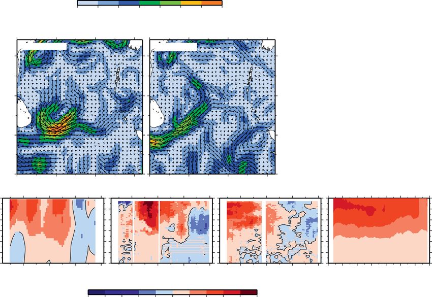
which provided a descrip- Fig. 2. R/V Sindhu Sadhana of CSIR National Institute of Oceanography, Goa,
tion of the annual cycle and India, which was used for the BoBBLE field program.
AMERICAN METEOROLOGICAL SOCIETY AUGUST 2018 | 1571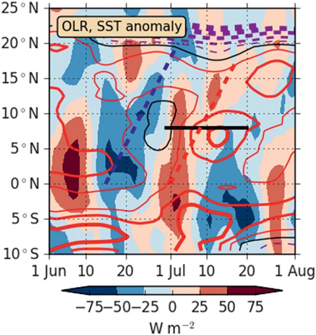
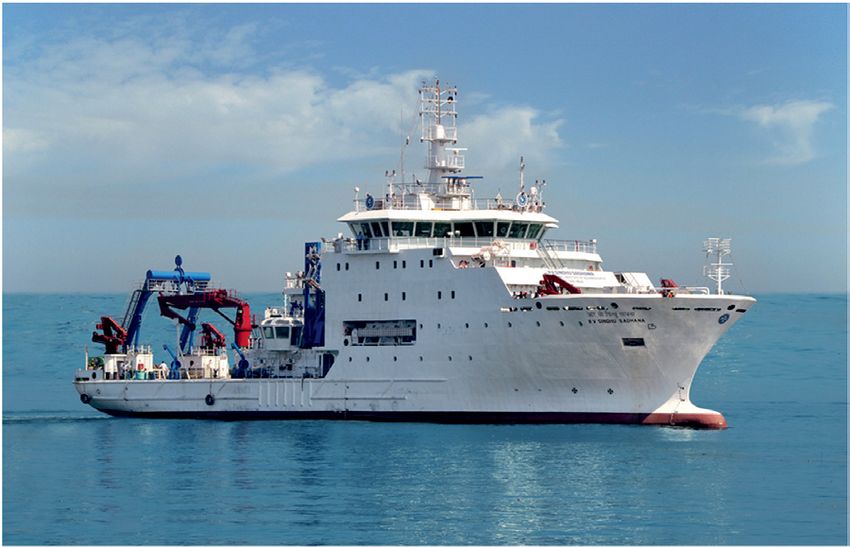
Fig . 3. (top) A map of the BoB and the cruise track
                                                                                   of the BoBBLE field program. SSS (shading) is from
20˚N                                                                               SMAP. (bottom) The section along which observations
            INDIA                                                                  were made during BoBBLE. The positions (black cir-
                                                                                   cles of TSW, Z1, Z2, Z3, and TSE) represent glider de-
                                BAY OF BENGAL
                                                                                   ployment locations (see Table 1 for details). Argo float
15˚N                                                                               deployments (see Table 2 for details), IOP, radiometer,
            Chennai                                                                and VMP profiling as well as water sampling were also
                                                                                   carried out at these locations. Stars indicate locations
                                                                                   where additional CTD profiles were measured during
10˚N                                 AR
                                                                                   the return leg of the cruise. At TSE, additionally, CTD
                                                                                   profiles were measured from 4 to 15 Jul 2016. Shading
                                TSW            TSE
                                                                                   indicates SST from Advanced Microwave Scanning
 5˚N                                                                               Radiometer for Earth Observing System (AMSR-E).

                                                                                   collected during the BoBBLE field program, the
         76˚E        80˚E     84˚E      88˚E         92˚E        96˚E      100˚E   details of which are given in the next section. The
                                                                                   “Meteorology and air–sea interaction” section and
       27       28      29      30      31     32           33      34       35
                                     SSS (PSU)                                     the “Oceanographic features of the southern BoB”
                                                                                   section describe air–sea interaction and the oceano-
                                                                                   graphic features of the southern BoB, respectively. We
                                                                                   conclude with a summary and outlook.
 9˚N

                                                                                   BoBBLE FIELD PROGRAM. The Research Vessel
 8˚N                                                                               (R/V) Sindhu Sadhana (Fig. 2) sailed from the port of
                      TSW Z1              Z2         Z3          TSE               Chennai, Tamil Nadu, India, on 24 June and returned
                                                                                   on 23 July 2016. The BoBBLE cruise was conducted
 7˚N
                                                                                   along the track shown in Fig. 3. Shipboard observa-
                                                                                   tions can be classified into two types: observations
 6˚N                                                                               made along the 8°N section from 85.3° to 89°E in the
   84˚E         85˚E         86˚E      87˚E          88˚E        89˚E      90˚E    international waters of the southern BoB and time
                                                                                   series observations were at 8°N, 89°E (referred to as
    28.8         29.0        29.2      29.4          29.6        29.8       30.0
                                      SST(oC)                                      TSE) for a period of 10 days, 4–15 July 2016. Ocean
                                                                                   glider deployments provided similar time series at
       monsoon. The overarching objectives of BoBBLE are                           locations marked as black circles in Fig. 3.
       to evaluate the role of ocean–atmosphere interac-                               Two shipboard ADCPs (operating at frequencies of
       tions in the simulation and prediction of the summer                        38 and 150 kHz), an automatic weather station (AWS),
       monsoon, to combine data and models to investigate                          and a thermosalinograph recorded data continuously
       the physical and biogeochemical processes under the                         during the cruise period. A Sea-Bird Electronics (SBE)
       monsoon forcing, and to determine the role of the                           911plus conductivity–temperature–depth (CTD)
       abovementioned processes in causing the synoptic-                           profiler measured vertical profiles and collected
       scale variability of the South Asian monsoon system.                        water samples at all points marked as stars in Fig. 3.
          The aim of this paper is to make the community                           Nominally, the casts were to a depth of 1,000 m.
       aware of the new dataset that has been acquired and                         At selected stations additional CTD casts extended
       to present a preliminary analysis of the observations                       all the way to the deep ocean floor. At TSE, CTD

 Table 1. Ocean glider deployments during the BoBBLE cruise. ID = identification.
 Glider ID            Waypoint                                     Deployed         Recovered     Instrumentation
    SG579             8°N, 86°E, then 8°N, 85°20´E                      30 Jun         20 Jul     CTD, dO2, Chl, backscatter, PAR
    SG534             8°N, 87°E                                          1 Jul         17 Jul     CTD, dO2, Chl, backscatter
    SG532             8°N, 88°E                                          2 Jul         16 Jul     CTD, dO2, Chl, backscatter
    SG620             8°N, 88°54´E                                       3 Jul         14 Jul     CTD, dO2, Chl, backscatter
     SG613            8°N, 89°06´E                                       4 Jul         15 Jul     CTD, microstructure shear, and temperature

1572 |           AUGUST 2018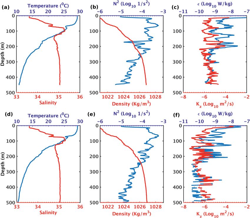
Table 2. Argo float deployments during the BoBBLE cruise.
No.    Argo float ID            Date       Time (UTC)         Lat (°N)    Lon (°E)     Notes
1      Navis OCR 0629       28 Jun 2016       1145              8          85.3        Daily profile surfacing at 1200 UTC
2      Apex STS 7599        30 Jun 2016       0910              8.04       86.05       Daily profile surfacing at 1500 UTC
3      Apex STS 7598        30 Jun 2016       0910              8.04       86.05       Daily profile surfacing at 0300 UTC
4      Navis OCR 0631        1 Jul 2016       1410              8.07       87.04       Daily profile surfacing at 1200 UTC
5      Apex STS 7597         1 Jul 2016       1410              8.07       87.04       Daily profile surfacing at 1500 UTC
6      Apex STS 7596         2 Jul 2016       0615              8          88          Daily profile surfacing at 1500 UTC
7      Navis OCR 0630        4 Jul 2016       1323              8.06       89.02       Daily profile surfacing at 1200 UTC

    observations were carried out to a depth of 500 m at      dataset covers a longer period than the BoBBLE field
    approximately 3-hourly intervals, with a once-daily       program, as there was a continuous Argo float pres-
    profile to 1,000 m. Four standard MetOcean drifting       ence in the BoB before the BoBBLE campaign, which
    buoys were also deployed during the BoBBLE field          was then significantly enhanced by the seven floats
    program.                                                  deployed during BoBBLE.
        Five ocean gliders were deployed during 1–19 July         To map mesoscale and submesoscale features,
    2016 along the 8°N transect (Table 1). All gliders        a Teledyne Oceanscience Underway CTD (uCTD),
    were equipped with a CTD package, enabling mea-           fitted with SBE conductivity–temperature (CT)
    surements of temperature and salinity with 0.5–1-m        sensors, was used for measuring temperature and
    vertical resolution from the surface to 1,000-m           salinity profiles while the ship was sailing at a speed
    depth. Four gliders were equipped with dissolved          of 6 kt (3.06 m s−1). Nominally, the uCTD probe was
    oxygen (dO2), chlorophyll fluorescence (Chl), and         allowed to profile vertically for 2 min in order to
    optical backscatter sensors. Additionally, one glider     achieve a drop rate of about 1.5–2.5 m s−1, covering
    (SG579) was equipped with a photosynthetically            a depth range of approximately 250 m, and the data
    active radiation (PAR) sensor, and another (SG613)        were binned at 1-m depth intervals.
    with microstructure shear and temperature sensors.            A vertical microstructure profiler (Rockland
    Individual dives lasted 3–4 h. In total, 462 dives were   Scientific VMP-250) comprising two shear probes,
    made. Optimally interpolated (OI) two-dimensional         one set of high-resolution microtemperature and
    (depth, time) gridded datasets (Matthews et al. 2014)     conductivity sensors and another set of standard
    were produced for each glider. The radii of influ-        CTD sensors, was operated at all glider stations along
    ence in the Gaussian weighting functions were 2 m         the transect as well as at TSE. At each station, two to
    and 3 h. The five depth–time OI datasets were then        three profiles were measured. At TSE, profiles were
    further combined into a single three-dimensional          measured at 0000, 0400, 0800, 1200, and 1700 UTC
    longitude–depth–time dataset, by linear interpola-        each day. In total, 138 casts were made, including
    tion in longitude, taking into account the movement       that at TSE.
    of the gliders with time.                                     To characterize the surface and subsurface light
        Seven Argo floats were deployed in the BoB along      field, bio-optical measurements were carried out with
    8°N, between 85.3° and 89°E (Table 2). As BoBBLE is       a Satlantic HyperPro II hyperspectral underwater ra-
    designed to target surface processes, all floats were     diometer (HUR) equipped with three sensors for light,
    programed to provide daily high-resolution profiles       an SBE Environmental Characterization Optics (ECO)
    of the top 500 m in a region where in situ surface data   triplet for fluorescence and colored dissolved organic
    are scarce. A second OI dataset was created using         matter (CDOM), and CTD sensors. The light sensors
    profiles from core Argo floats from the international     measured downwelling, upwelling, and total solar
    Argo program, BoBBLE Argo floats, glider profiles,        irradiance. The HUR was operated for 17 days under
    and the shipboard CTD. These OI data were mapped          cloud-free conditions between 0600 and 0700 UTC at
    using World Ocean Database climatology (Boyer             TSE, and along the 8°N transect between 0530 and
    et al. 2013) and gridded at 25 longitude grid points      0800 UTC. A total of 37 profiles were collected during
    at 8°N, from 83° to 95°E at 0.5° intervals. The time      BoBBLE. An inherent optical profiler (IOP) was used
    grid ran from 1 June 2016, before the BoBBLE field        for the measurement of light absorption and scattering
    campaign started, to 30 September 2016, with data         coefficients, backscattering coefficient, chlorophyll-a,
    from each day gridded separately. This combined OI        CDOM, turbidity, and PAR along with a CTD sensor.

    AMERICAN METEOROLOGICAL SOCIETY                                                              AUGUST 2018          | 1573
The IOP was operated at          Table 3. Details of shipboard meteorological instruments. Surface vari-
     TSE at 0130 and 0830 UTC         ables, including air temperature, SST, relative humidity, pressure, and
     each day.                        all four components of radiation, wind speed and direction, rain rate, and
         The meteorologica l          ship position, were continuously monitored by the AWS. Surface variables
     measurements includ-             were sampled at 10-s intervals, and 1-min averages (including true wind
     ed an AWS, an air–sea            speed and direction) were stored. The ship’s SBE SST sensor was placed at
                                      a depth of approximately 3.5 m below sea level (Weller et al. 2008).
     f lux obser ving system
     (Table 3), a nd rad io-          Parameter                               Range            Mean accuracy Resolution
     sondes. A LI-COR infra-          Wind speed (R. M. Young)                0.7–50 m s−1     0.2 m s−1 or 2% 0.1 m s−1
     red gas analyzer in con-         Wind direction (R. M. Young)            0°–360°                 3°           1°
     junction with the 3D sonic       Air temperature (YSI)                   0°–45°C               0.2°C       0.05°C
     anemometer–based eddy
                                      Relative humidity (Rotronic)            0%–100%                2%          0.5%
     covariance system and
                                      Atmospheric pressure (Honeywell)        850–1,050 hPa        0.1 hPa     0.01 hPa
     high-frequency response
                                                                                         −1                 −1
     ship motion sensors were         Optical rain gauge (Optical Scientific) 0–50 mm  h         0.4 mm   h    0.25  mm
                                                                                            −1
     installed at the bow, at a       Radiation (shortwave) (LI-COR)          0–300 mW cm            5%           —
     height of approximately          SST (SBE)                               0°–35°C                0.1°       0.05°C
     15 m above the sea surface
     and 6 m above the fore-
     castle deck. Sensible and latent turbulent heat fluxes 2003). Upper-air observations of temperature, pres-
     are estimated using the eddy covariance method sure, humidity, and wind were taken with Vaisala
     (Fairall et al. 1997; Edson et al. 1998; Dupuis et al. RS92 radiosondes, launched nominally at 0000 and
                                                                  1200 UTC every day. Additional launches were also
                                                                  made on some days to capture the diurnal cycle.

                                                                METEOROLOGY AND AIR–SEA INTER-
                                                                ACTION. Large-scale conditions over the BoB during
                                                                summer 2016. The all-India rainfall for 2016 had a
                                                                3% deficit relative to climatology (www.imd.gov.in),
                                                                ENSO conditions were near neutral, and SST anoma-
                                                                lies in the tropical Pacific and Indian Oceans were
                                                                modest (www.ospo.noaa.gov). The Indian Ocean
                                                                dipole (Saji et al. 1999) was in a negative state, with
                                                                slightly warmer-than-usual conditions in the eastern
                                                                Indian Ocean and cooler-than-usual conditions in
                                                                the west, representing an intensification of the usual
                                                                cross-basin gradient. Despite this, 2016 can be seen
                                                                as a representative monsoon season and is therefore
                                                                ideally suited for investigating its link with conditions
                                                                in the BoB.
                                                                    The mean monsoon winds during the observa-
                                                                tion period were steady southwesterlies (Fig. 1d)
                                                                and the SMC was intense with an axis oriented in
Fig. 4. Hovmöller diagram (averaged from 80° to 95°E) for       the southwest–northeast direction, to the east of Sri
anomalous 5-day running mean outgoing longwave radia-           Lanka (Fig. 1c). The mean SST was relatively cooler
tion (OLR; shading interval: 25 W m−2), SST (line contour       around the SMC with warmer water farther to the
interval: 0.2°C; negative contours: dashed purple, zero         west and east. The east–west SST contrast that is
contour: solid black, positive contours: solid red). The line   typically seen in the climatology (Fig. 1a) was not
at 8°N shows the timing of the BoBBLE ship and glider and       as well developed during the period of observations
Argo float deployments (solid black). Negative (positive)
                                                                (Fig. 1c). The mean SSS pattern was comparable to
OLR anomalies indicate convectively active (suppressed)
phase of BSISO. The main axis of northward propagation          climatology (Figs. 1b,d).
of the active (dashed blue) and suppressed (dashed red)             Intraseasonal variability had a significant effect
phases of the BSISO during Jun–Jul 2016.                        on the conditions observed during the BoBBLE

1574 |      AUGUST 2018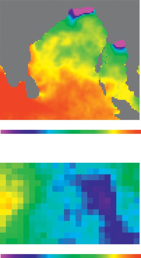
campaign. In June 2016 the
southern BoB was under the
influence of a convectively
active phase (Fig. 4) of the
boreal summer intraseason-
al oscillation (BSISO) (Lee
et al. 2013). This propagated
northward (dashed blue line
in Fig. 4) and was replaced
by a convec t ively sup-
pressed phase of the BSISO
during July 2016. Toward
the end of the deployment,
conditions returned to the
convectively active phase
with the incursion of the
next cycle of the BSISO.
Hence, the main BoBBLE
deployment sampled the
transition between the end
of one active BSISO event,
the subsequent suppressed
phase, and the initiation of
the active phase in the fol-
lowing BSISO event. This is
an ideal framework for ana-
lyzing the high-resolution
in situ observations made
during the BoBBLE cruise.

In situ measurements of air–
sea interaction. The time
series of surface fluxes and
atmospheric and ocean sur-
face conditions observed
from the ship are described
here, within the large-scale
context of the suppressed
phase of the BSISO in the
southern BoB. The focus
is on the period 4–15 July       Fig. 5. (a) Ship position as a function of time. Latitude (red line) and longitude
2016 when the ship was at        (blue line) are marked. The double-headed arrow shows the time series ob-
TSE (Fig. 5a). During this       servation period at TSE (8°N, 89°E). (b) SST from AWS and CTD at 3.4-m
period no precipitation was      depth. (c) Air temperature. (d) Surface (approximately 10 m) wind speed
observed. Cloud conditions       (red line) and radiosonde wind speed (black squares) at 975 hPa. (e) Surface
                                 net heat flux into the ocean. RS is radiosonde, Ta-sonic is sonic anemometer
were characterized by bro-
                                 temperature corrected for water vapor, and ECM and BM refer to turbulent
ken layers of mid- and high-     fluxes calculated using the eddy covariance and bulk methods, respectively;
level clouds and scattered       refer to text for other abbreviations.
small cumulus, with a gener-
ally high surface solar radia-
tion flux. The surface wind speeds during the first half in the latter half of the period, they decreased to 5 m s−1
of the period were 8–10 m s−1 (Fig. 5d), typical for the or below, with an associated reduction in the (cooling)
southern BoB during the summer monsoon. However, surface latent heat flux.

AMERICAN METEOROLOGICAL SOCIETY                                                            AUGUST 2018        | 1575
The high solar radiation flux and relatively low   the BSISO (Lee et al. 2013). Consequently, the net heat
     latent heat flux are consistent with conditions that  flux into the ocean was positive (Fig. 5e). This led to a
     prevail during the suppressed (calm, clear) phase of  steady increase in SST, from 28.0° to 29.5°C (Fig. 5b),
                                                                                     again consistent with the
                                                                                     developing oceanic condi-
                                                                                     tions typically found in the
                                                                                     suppressed BSISO phase.
                                                                                     Surface atmospheric tem-
                                                                                     perature (Fig. 5c) increased
                                                                                     in pace with the SST.
                                                                                         Deep atmospheric con-
                                                                                     vection broke out at the end
                                                                                     of the TSE period. From 16
                                                                                     July 2016 onward, deep con-
                                                                                     vective cloud systems with
                                                                                     intense precipitation, asso-
                                                                                     ciated with the next active
                                                                                     BSISO phase, were observed
                                                                                     from the ship. It should be
                                                                                     noted that at this time, the
                                                                                     ship had departed TSE and
                                                                                     was cruising westward on
                                                                                     the return leg of the 8°N
                                                                                     section (Fig. 5a); hence, the
                                                                                     sampling of these precipitat-
                                                                                     ing systems was not at a fixed
                                                                                     location. This deep convec-
                                                                                     tion was part of the next
                                                                                     active BSISO phase (Fig. 4).
                                                                                         The change in atmo-
                                                                                     spheric characteristics from
                                                                                     suppressed to active convec-
                                                                                     tion can clearly be seen in
                                                                                     the shipboard AWS time
                                                                                     series. The most notable
                                                                                     change is that air temper-
                                                                                     ature dropped on 15 July
                                                                                     and remained significantly
                                                                                     lower than SST from then
                                                                                     on (Figs. 5b,c). The air tem-
                                                                                     perature was much more
                                                                                     variable, with spikes of low
                                                                                     temperature followed by
                                                                                     a gradual recovery. Low-
                                                                                     temperature spikes are due
                                                                                     to evaporation from falling
                                                                                     raindrops in the subcloud
                                                                                     layer and formation of a pool
Fig. 6. (a) Longitude–time section of OI glider temperature at 1-m depth.            of cold air near the surface
The longitudes of the five gliders are shown (colored lines). (b) Average di-
                                                                                     (i.e., wet-bulb effect). Surface
urnal cycle of temperature for glider SG579 at the western end of the 8°N
section. Time of day is in local solar time (LST). (c) Longitude–time section        wind speed increases from
of temperature at 1-m depth for Jul–Sep 2016, based on OI Argo data. A               its minimum on 15 July
3-day moving mean has been applied to the Argo data.                                 (Fig. 5d) and shows large

1576 |      AUGUST 2018
Fig. 7. Sri Lanka dome. (a) AVISO MSLA (cm) for 30 Jun 2016 (contours) and wind stress curl (shading, N m−3)
from ASCAT averaged for the period 20 Jun–1 Jul 2016. (b) AMSR-E SST (shading, °C) averaged for the period
27–30 Jun 2016 overlayed on current vectors (m s −1) from OSCAR for 2 Jul 2016. (c) Temperature and (d) salinity
profiles that contrast the spatial structure of the SLD. Profiles were measured at a location to the north (black)
and east of the SLD (green), and inside the SLD (blue, red). Refer to Fig. 3 for the locations. Salinity profiles
show that the high-salinity core of the SMC (green curve) is absent in the regions of the SLD (blue and red).
variability. These are also likely due to gusts of cold, decreased (Fig. 6c) followed by a weaker warming from
dry air originating from the convective systems associ- mid-August to mid-September and a further cooling.
ated with the transition to an active phase of BSISO.
Overall, the shipboard measurements com OCEANOGRAPHIC FEATURES OF THE
prehensively captured the transition from the SOUTHERN BoB. The deployment of multiple
atmospheric convectively suppressed phase of the platforms has yielded an unprecedented description
BSISO during 4–15 July to the following convectively of the oceanographic features of the southern BoB
active phase. during the summer monsoon. In particular, a nearly
Glider measurements extend the analysis of one-month time series of physical and biogeochemi-
air–sea interaction along the entire 8°N section. The cal variables along a zonal section at 8°N has been
longitude–time section of ocean temperature at 1-m obtained. This section describes these features briefly.
depth (Fig. 6a) clearly shows the gradual warming
across the whole section from approximately 28.5°C SLD. The cyclonic circulation feature located to the east
on 3 July to up to 30.5°C on 13 July. Superimposed of Sri Lanka, caused by cyclonic wind stress curl above
on this are strong diurnal fluctuations, especially at the Sri Lanka dome (SLD; Fig. 7a), which is associated
the westernmost glider (SG579) and 88°E (SG532). with the doming of the thermocline (Vinayachandran
These represent the formation of surface diurnal and Yamagata 1998; Wijesekera et al. 2016a). The SLD
warm layers (Fig. 6b) that were previously diagnosed during BoBBLE is seen as a patch of negative mean
in the Indian Ocean by an ocean glider (Matthews sea level anomalies (MSLA; Fig. 7a), enclosed by the
et al. 2014). zero MSLA contour (thick line). The SLD was well
Argo floats extend the analysis even further to the developed during the survey with cyclonic circulation
end of the season. With the onset of the next active and cooler SST around it (Fig. 7b). The CTD profiles
phase of BSISO in mid-July, the temperature rapidly measured during BoBBLE captured the doming of the
AMERICAN METEOROLOGICAL SOCIETY AUGUST 2018 | 1577Fig . 8. Longitude–depth sections of temperature along 8°N using (a) CTD section during 30 Jun– 4 Jul 2016,
(b) glider data on 8 Jul 2016, (c) CTD section observed during 15–20 Jul 2016, and (d) OI Argo data on 24 Jul 2016.
thermocline with respect to its exterior. On 28 and 30 westward as the season progresses (Fig. 8c). It has
June 2016, CTD profiles were measured at locations been possible to delineate the changes in the east–
within the SLD, and on 1 July 2016 on its outer edge. west slope of the thermocline from early to mid-July
A comparison of these profiles shows that the thermo- because of these datasets generated by multiple in-
cline (taken as the depth of the 20°C isotherm; D20) struments (Fig. 8d).
within the dome is about 30 m shallower compared
to its exterior (Fig. 7c). The dome also shows distinct The summer monsoon current. The SMC flows east-
salinity characteristics (Fig. 7d). The subsurface high- ward to the south of India (Schott et al. 1994) and
salinity core that exists along with the SMC (see “The then turns to flow into the BoB (Murty et al. 1992;
high-salinity core” section) does not penetrate into the Vinayachandran et al. 1999, 2013). The SMC was
SLD. The near-surface salinity within the SLD is higher fully developed during the observation period with
compared to the north but lower than that in the east, near-surface speeds of 0.5–1 m s−1 (Figs. 9a,b). The
confirming its isolation from the influence of the SMC. circulation was characterized by a large cyclonic gyre
Along 8°N (Fig. 8), the thermocline (D20) within to the east of Sri Lanka that was fully developed by the
the dome is elevated relative to the region to the east. last week of June (Fig. 9a). The main axis of the SMC
The CTD and glider sections in early July (Figs. 8a,b) that flows northeastward into the BoB weakened and
correspond well during the season. The SLD moves moved westward by mid-July; in the process, the gyre
▶ Fig. 9. The SMC. Surface currents from OSCAR (vector, m s−1) overlaid on current speed (shading) on (a) 26
Jun and (b) 17 Jul 2016. (c) Trajectories of four drifting buoys deployed during the cruise. (d) Meridional geo-
strophic current referenced to 500 dbar, calculated using ship CTD salinity measured at every 25° longitude
along 8°N during 15–20 Jul 2016. (e) Meridional current measured using the ADCP during 30 Jun–4 Jul, and (f)
15–20 Jul 2016. (g) Time–depth meridional geostrophic current referenced to 500 dbar, at a nominal longitude
of 87.5°E, calculated using SG534 and SG532 glider data (Table 1).
1578 | AUGUST 2018AMERICAN METEOROLOGICAL SOCIETY AUGUST 2018 | 1579
Fig. 10. High-salinity core. (a) Vertical section of CTD
salinity along 8°N, measured during 30 Jun–4 Jul 2016,
at stations located 1° apart between 85.3° and 89°E.
(b) As in (a), but profiled during 15–20 Jul 2016 at stations
located 25° longitude apart. (c) Time–depth section of
salinity measured at TSE during 4–15 Jul 2016. High-
salinity (>35) core (contours) in (a)–(c). (d) Time–longi-
tude section of salinity averaged between 90 and 130 m
using glider data. (e) Time–longitude section of salinity
averaged between 90 and 130 m using Argo data.
elongated and shrank. Multiple filaments emanated was restricted to depths shallower than 200 m, in
from the SMC in different directions (Fig. 9b). One of agreement with previous observations (Wijesekera
them flowed toward the equator, another toward the et al. 2016a). ADCP profiles confirm the shallow na-
east, one toward the northeast, and another continued ture of the SMC (Figs. 9e,f). Between the two visits,
to the southeast. One of the drifting buoys deployed the SMC weakened and shifted westward, the latter
during the cruise at TSW (8°N, 85.3°E) Fig. 3) on 29 being consistent with the well-known process of
June traversed along the cyclonic gyre (Fig. 9c) but Rossby wave propagation across the BoB (McCreary
two drifters continued toward India. The drifter de- et al. 1996; Shankar et al. 2002). There is remarkable
ployed in the east (147132; Fig. 9c) moved southeast. agreement between the ADCP data and geostrophic
The BoBBLE section cut across the main branch currents. The time–depth section of the geostrophic
of the SMC, and the TSE location was located on the comp onent of the SMC derived from glider data
outer edge of the filament flowing to the northeast. (Figs. 9e,g) shows decreasing velocities, consistent
Geostrophic currents (Fig. 9d) showed high speeds with the weakening and westward propagation of
(>0.5 m s–1) near the surface and the northward flow the SMC.
1580 | AUGUST 2018Fig. 11. Changes in the temperature and salinity characteristics of the upper layer due to freshening. (top) First
freshening event (4–6 Jul 2016) described in the text. (bottom) Second freshening event (7–13 Jul 2016). Curves
in all panels indicate temperature (red), salinity (blue), density (black), and MLD (horizontal lines). The date
and time (UTC) of each profile is given above the respective panel. The situation (left) before and (middle)
during the freshening event, and (right) the peak of the freshening event.
The high-salinity core. The SMC carries high-salinity 100 m on 15 July, suggesting a steady supply of high-
water (>35.2 psu) from the Arabian Sea into the BoB. salinity water during the observation period. Glider
On encountering the lighter water of lower salin- (Fig. 10d) and Argo (Fig. 10e) observations reveal
ity, the Arabian Sea Water subducts beneath the temporal variations of the high-salinity core along
latter. The intrusion of high-salinity (35–35.6 psu) the 8°N section.
water occurs below the mixed layer, to a maximum
depth of about 200 m (Fig. 10). During 30 June–4 Freshening events and barrier-layer formation. The
July (Fig. 10a), the high-salinity core was confined 10-day time series at TSE captured two freshening
to 86°–89°E, between 25 and 175 m depth. At the events, one during 4–6 July and the other during
eastern end (at 89°E), the core thinned to about 25 m 8–9 July (Fig. 10c). These events led barrier layers to
thick. In contrast, at the western end, the profiles form between the base of the upper isohaline layer
measured inside the SLD did not show the presence and the base of the isothermal layer. The barrier layer
of Arabian Sea Water (Fig. 7d). At TSE, (Fig. 10b) the formed rapidly during the first event. The SSS on 4
core thickened from about 25 m on 4 July to about July dropped by 0.3 in 2 h, decreasing from 34.3 psu
AMERICAN METEOROLOGICAL SOCIETY AUGUST 2018 | 1581at 0530 UTC to 33.9 psu by 0730 UTC (Fig. 11). Since shallowing and barrier-layer formation occur to a
there was no rain locally, this drop in salinity is at- comparable degree, suggesting that the behavior of
tributed to horizontal advection. The mixed layer the southern BoB mixed layer is comparable to that
depth (MLD) decreased from 70 to 18 m, leading to of the north during the summer monsoon.
the formation of a barrier layer that was about 50 m
thick and had a temperature of 29°C. The upper layer Submesoscale observations. A uCTD was used for
warmed by about 0.3°C relative to the barrier layer measuring vertical profiles of temperature and sa-
below, during the following diurnal cycle. linity while the ship was in transit (details are in the
The second event occurred more gradually; the “BoBBLE field program” section). A uCTD section
SSS (MLD) decreased from 34.40 psu (75 m) on 7 July measured just after a spell of rain near TSE on 15
to 33.57 psu (35 m) on 13 July (Fig. 11). Consequently, July 2016 (Fig. 12a) captured the spatial scale of a
a new barrier layer formed that was about 40 m thick. low-salinity pool that formed as result of the rain
Periods of low SST coincided with higher salinity and event. The salinity within the fresh pool was lower
the SST increased after both freshening events. There by 0.1 psu compared to the region outside, and the
was also a distinct increase in the diurnal warming impact of rain was seen to a depth of 12 m. The width
of SST after the freshening. of this pool was 7 km. There was no apparent change
The barrier-layer formation at TSE is comparable in the temperature (Fig. 12b), and the isothermal layer
to that in the northern bay, where the influence of extended all the way to about 40 m despite the isoha-
river runoff and rainfall is more intense. Subsequent line layer being confined to the upper 10 m.
to the arrival of a fresh plume, the MLD decreased
from 30 to 10 m during the 1999 summer monsoon Microstructure measurements. Previous indirect dis-
(Vinayachandran et al. 2002), as a result of the de- sipation measurements inferred from Argo floats
crease in SSS by about 4 psu over a period of 7 days. in the central BoB suggested very low dissipation
Observations during 2009 (Rao et al. 2011) also rates in the 250–500-m-depth range (Whalen et al.
showed a similar decrease of SSS and MLD in one 2012). Recent direct dissipation measurements in the
day. It is quite remarkable that even in the southern northern and central BoB (Jinadasa et al. 2016) show
bay, where the direct influence of freshwater is much that the pycnocline is mostly decoupled from the
weaker compared to that in the north, the mixed layer low-salinity surface layer, with low turbulence in the
Fig. 12. uCTD observations of a rain-formed low-salinity pool. (a) Salinity along a 14-km section over which 21
vertical profiles were measured just after a spell of rain. Locations of uCTD profiles are indicated using aster-
isks marked at a depth of 55 m. Along the depth axis, the raw data are averaged into 1-m bins before plotting.
(b) Vertical profiles of temperature (black) and salinity (blue) measured outside (at x = 2 km, thick lines) and
inside (at x = 6 km, thin lines) the low-salinity pool.
1582 | AUGUST 2018deeper layer. Profiles from simultaneous casts of the and Kz were greater than 10 –8 W kg–1 and 10 –4 m2 s–1,
VMP-250 (Figs. 13a–c) and the microstructure glider respectively. Below the mixed layer, ε decreased to
(Figs. 13d–f) at locations separated by a few kilome- 10 –10 W kg–1 and Kz reduced to 10 –6 m2 s–1. The micro-
ters suggest a shallow mixed layer (approximately 20 structure data are consistent with the observations of
m thick) and a freshened upper layer (33.5 psu) com- Jinadasa et al. (2016) and Whalen et al. (2012).
pared to the thermocline region, where the salinity
is 35.25 psu, confirming that the two platforms are Biogeochemical observations. Light penetration and
sampling similar water columns. The 3-m binned chlorophyll . The glider SG579 (Table 1) equipped
profiles of turbulent kinetic energy dissipation rate with a PAR sensor provides a proxy for the shortwave
ε and vertical diffusivity Kz from the VMP (Fig. 13c) radiation flux. A sample profile (Fig. 14) shows a rapid
and the microstructure glider (Fig. 13f) suggest a decrease in radiation flux in the top 1–2 m, associ-
sporadic and intermittent nature of the mixing in ated with the absorption of the red light part of the
the water column. Within the mixed layer, the ε spectrum. Below this level PAR decreases much more
Fig. 13. Data from VMP-250 at 7°54'N and 89°06'E on 15 Jul 2016: (a) temperature (blue) and salinity (red), (b)
squared Brunt–Väisälä frequency (blue) and density (red), and (c) log10 of ε (blue) and log10 of K z (red). Near-
simultaneous data from glider SG613: (d) temperature (blue) and salinity (red), (e) N 2 (blue) and density (red),
and (f) log10 of ε (blue) and log10 of K z (red). The noise threshold of ε = 10 –10.5 W kg −1. The measured microstruc-
ture shear was used to infer ε and K z in the water column by assuming isotropic turbulence (Moum et al. 1995)
and a mixing efficiency of 0.2 (Osborn 1980). The upper 10 m of the VMP-250 data has been removed to avoid
contamination by the ship’s wake.
AMERICAN METEOROLOGICAL SOCIETY AUGUST 2018 | 1583slowly, associated with the absorption of the blue light high pCO2 compared to the atmospheric mixing
part of the spectrum. A double exponential curve was ratios, suggesting that the southern BoB is a possible
fitted, producing a scale depth of 0.3 m for red light, source of CO2 to the atmosphere during summer.
and 18 m for blue light. Collocated measurements of
chlorophyll concentration (Table 1) show a layer of SUMMARY AND OUTLOOK. During a typical
chlorophyll below 30 m (green line in Fig. 14), with summer monsoon season, discrete cloud bands peri-
near-zero values above this. The effects of chlorophyll odically form over the Indian Ocean and then migrate
absorption of solar radiation, and any subsequent ef- over the Asian landmass, culminating in rainfall
fect on SST, and through ocean–atmosphere interac- there. Such cloud bands can be embedded in large-
tions, a feedback onto precipitation, will be examined scale intraseasonal oscillations or manifest as synop-
during the project. tic monsoon depressions. The BoB is a key region for
the formation and propagation of these atmospheric
O2 and pCO2 . The dissolved oxygen at the surface systems. Thus, the variability of rainfall over the
ranged between 199 and 212 μmol kg−1 with the Asian landmass during the monsoon is closely linked
eastern part of the transect showing relatively higher to the exchange of heat and moisture taking place over
values (Fig. 15a). The surface pH (Fig. 15b), total the Indian Ocean. Hence, understanding the detailed
alkalinity (Fig. 15c), and partial pressure of CO2 physical processes of ocean–atmosphere interaction
(pCO2; Fig. 15e) exhibited a similar distribution. over the Indian Ocean, and the BoB in particular, is
The pH had a range of 8.071–8.168 units, whereas crucial for understanding and the successful model-
total alkalinity varied between 2,172 and 2,295 µmol ing and prediction of monsoon variability.
kg−1. Atmospheric CO2 (pCO2air) ranged between 386 BoBBLE was motivated by this need and was de-
and 409 µatm (Fig. 15d), where higher concentra- signed to investigate oceanographic conditions and
tions were associated with the station at 10°N, 85.3°E air–sea interaction over the hitherto little-known
(Fig. 3). This station also exhibited high pCO2 (pCOsw
2
) southern BoB during the summer monsoon. This pa-
with a range of 467–554 µatm. The low surface pH in per outlines the preliminary results from the BoBBLE
tandem with low alkalinity and high pCO2 at this sta- field program, which was aimed at collecting high-
tion suggest upwelled waters, presumably associated quality in situ observations from multiple platforms,
with the SMC. Overall, all sampling stations exhibited including an ocean research ship, five ocean gliders,
and seven specially config-
ured Argo floats.
The BoBBLE observa-
tions were made during July
2016, during a suppressed
phase of the BSISO when
the ocean and atmosphere
were being preconditioned
for an impending active
stage of the monsoon. Dur-
ing this period, which was
characterized by intense
solar radiation, the ocean
wa rmed a nd ex hibited
strong diurnal variability.
At the end of the BoBBLE
observation period, atmo-
spheric convection broke
out over the southern BoB
as part of the next, active
phase of a northward-prop-
agating BSISO. This active
Fig. 14. PAR profile (black dots) from a sample dive from glider SG579, near phase subsequently led to
midday on 6 Jul 2016. The best-fit double exponential curve is shown by the rainfall over India and the
black line. Chlorophyll concentration is shown by the green crosses and line. Asian landmass.
1584 | AUGUST 2018Fig. 15. Spatial variation of surface biogeochemical properties during BoBBLE: (a) dissolved oxygen; (b) pH; (c) total
alkalinity; and (d) pCO2air, pCO2sw, and the difference in air–sea pCO2 concentration. Water sampling was carried
out using an SBE CTD–rosette system fitted with 10-L Niskin bottles. Samples were collected along the 8°N
transect at locations (red stars) denoted in Fig. 3
The BoBBLE campaign has also made detailed of Earth Sciences, government of India, under its Monsoon
observations of the major oceanographic features of Mission program administered by the Indian Institute of
the southern BoB. Using multiple in situ platforms, Tropical Meteorology, Pune. We are indebted to the CSIR
the spatial and temporal evolution of features such as National Institute of Oceanography, Goa, India, for pro-
the SLD and the high-salinity core in the SMC have viding the R/V Sindhu Sadhana for BoBBLE. We greatly
been delineated using in situ datasets. Other obser- appreciate the encouragement by Dr. M. Rajeevan, secretary
vations include the formation of barrier layers in the of MoES, and Dr. S. S. C. Shenoi, director of INCOIS, and
southern BoB and details of the associated changes the support and cooperation of Dr. P. S. Rao (NIO) and the
in the mixed layer. The physical processes involved in captain, officers, and crew of the R/V Sindhu Sadhana. We
barrier-layer formation in the southern BoB contrast thank Dr. D. Shankar (NIO), Dr. R. Venkatesan (NIOT), Dr.
with those at work in the north. Tata Sudhakar (NIOT), Dr. Anil Kumar (NCOAR), Dr. M.
The next challenge for the BoBBLE program is to Ravichandran (INCOIS), and their team, for their support
incorporate the observational knowledge gained by for the field program. ASCAT wind data were obtained
the field program into physical process models and from IFREMER (www.ifremer.fr/cersat/en/data/data.htm);
to determine the sensitivity of the monsoon system to NCEP data from NOAA (www.esrl.noaa.gov/psd/; Kalnay
ocean–atmosphere interactions in the southern BoB. et al 1996); CERES downward longwave and shortwave
radiation data from NASA (https://ceres.larc.nasa.gov);
ACKNOWLEDGMENTS. BoBBLE is a joint MoES, OSCAR data from NASA (https://podaac.jpl.nasa.gov
India–NERC, U.K. program. The BoBBLE field program on /CitingPODAAC); AMSR-E products from Remote Sensing
board the R/V Sindhu Sadhana was funded by the Ministry Systems (www.remss.com/missions/amsr); KALPANA OLR
AMERICAN METEOROLOGICAL SOCIETY AUGUST 2018 | 1585from the Indian Institute of Tropical Meteorology (www Gadgil, S., 2003: The Indian monsoon and its variability.
.tropmet.res.in); TRMM rainfall data from NASA (http:// Annu. Rev. Earth Planet. Sci., 31, 429–467, https://doi
daac.gsfc.nasa.gov/precipitation); MSLA from Copernicus .org/10.1146/annurev.earth.31.100901.141251.
Marine and Environment Monitoring Service (CMEMS; Jain, V., and Coauthors, 2017: Evidence for the existence
http://marine.copernicus.eu/); gridded Argo data from the of Persian Gulf Water and Red Sea Water in the Bay
Global Data Assembly Centre (Argo GDAC); and SEANOE of Bengal. Climate Dyn., 48, 3207–3226, https://doi
and ERA winds, fluxes, and meteorological parameters from .org/10.1007/s00382-016-3259-4.
ECMWF (www.ecmwf.int/en/research/climate-reanalysis Jinadasa, S. U. P., I. Lozovatsky, J. Planella-Morató, J. D.
/era-interim). The core Argo profiles were collected and Nash, J. A. MacKinnon, A. J. Lucas, H. W. Wijesekera,
made freely available by the international Argo program and H. J. S. Fernando, 2016: Ocean turbulence and
and the national programs that contribute to it (www.argo mixing around Sri Lanka and in adjacent waters of
.ucsd.edu, http://argo.jcommops.org). NPK was supported the northern Bay of Bengal. Oceanography, 29 (2),
by NERC (NE/L010976/1). ASF, BGMW, and SCP were sup- 170–179, https://doi.org/10.5670/oceanog.2016.49.
ported by the NERC BoBBLE project (NE/L013835/1, NE/ Joseph, P. V., K. P. Sooraj, C. A. Babu, and T. P. Sabin,
L013827/1, NE/L013800/1). PNV was supported by the Min- 2005: A cold pool in the Bay of Bengal and its interac-
istry of Earth Sciences (MM/NERC-MoES-02/2014/002). tion with the active-break cycle of monsoon. CLIVAR
Participation of all Indian scientists were supported by the Exchanges, No. 34, International CLIVAR Project
MoES-BoBBLE project, and all others were supported by Office, Southampton, United Kingdom, 10–12.
the NERC-BoBBLE Project. We thank three anonymous Kalnay, E., and Coauthors, 1996: The NCEP/NCAR
reviewers for their thoughtful and constructive comments 40-Year Reanalysis Project. Bull. Amer. Meteor.
on the manuscript. Soc., 77, 437–471, https://doi.org/10.1175/1520-0477
(1996)0772.0.CO;2.
Lee, C. M., and Coauthors, 2016: Collaborative obser-
REFERENCES vations of boundary currents, water mass variabil-
Bhat, G. S., and R. Narasimha, 2007: Indian summer ity, and monsoon response in the southern Bay of
monsoon experiments. Curr. Sci., 93, 153–164. Bengal. Oceanography, 29 (2), 102–111, https://doi
—, and Coauthors, 2001: BOBMEX: The Bay of .org/10.5670/oceanog.2016.43.
Bengal Monsoon Experiment. Bull. Amer. Meteor. Lee, J.-Y., B. Wang, M. C. Wheeler, X. Fu, D. E. Waliser,
Soc., 82, 2217–2243, https://doi.org/10.1175/1520 and I.-S. Kang, 2013: Real-time multivariate indices
-0477(2001)0822.3.CO;2. for the boreal summer intraseasonal oscillation
Boyer, T. P., and Coauthors, 2013: World Ocean Data- over the Asian summer monsoon region. Climate
base 2013. NOAA Atlas NESDIS 72, 209 pp. Dyn., 40, 493–509, https://doi.org/10.1007/s00382
Das, U., P. N. Vinayachandran, and A. Behara, 2016: -012-1544-4.
Formation of the southern Bay of Bengal cold pool. Matthews, A. J., D. B. Baranowski, K. J. Heywood, P. J.
Climate Dyn., 47, 2009–2023, https://doi.org/10.1007 Flatau, and S. Schmidtko, 2014: The surface diurnal
/s00382-015-2947-9. warm layer in the Indian Ocean during CINDY/
Dupuis, H., C. Guerin, D. Hauser, A. Weill, P. Nacass, DYNAMO. J. Climate, 27, 9101–9122, https://doi
W. M. Drennan, S. Cloché, and H. C. Graber, 2003: .org/10.1175/JCLI-D-14-00222.1.
Impact of f low distortion corrections on turbu- —, and Coauthors, 2015: BoBBLE: Bay of Bengal
lent f luxes estimated by the inertial dissipation boundary layer experiment. CLIVAR Exchanges, No.
method during the FETCH experiment on R/V 68, International CLIVAR Project Office, Southamp-
L’Atalante. J. Geophys. Res., 108, 8064, https://doi ton, United Kingdom, 38–42.
.org/10.1029/2001JC001075. McCreary, J. P., W. Han, D. Shankar, and S. R. Shetye,
Edson, J. B., A. A. Hinton, K. E. Prada, J. E. Hare, and 1996: Dynamics of the East India Coastal Cur-
C. W. Fairall, 1998: Direct covariance flux estimates rent: 2. Numerical solutions. J. Geophys. Res., 101,
from mobile platforms at sea. J. Atmos. Oceanic 13 993–14 010, https://doi.org/10.1029/96JC00560.
Technol., 15, 547–562, https://doi.org/10.1175/1520 McPhaden, M. J., and Coauthors, 2009: R AMA:
-0426(1998)0152.0.CO;2. The Research Moored Array for African–Asian–
Fairall, C., A. White, J. Edson, and J. Hare, 1997: Integrat- Australian Monsoon Analysis and Prediction.
ed shipboard measurements of the marine boundary Bull. Amer. Meteor. Soc., 90, 459–480, https://doi
layer. J. Atmos. Oceanic Technol., 14, 338–359, https:// .org/10.1175/2008BAMS2608.1.
doi.org/10.1175/1520-0426(1997)0142.0.CO;2. Comparison of turbulence kinetic energy dissipation
1586 | AUGUST 2018rate estimates from two ocean microstructure profil- —, Y. Masumoto, T. Mikawa, and T. Yamagata, 1999: ers. J. Atmos. Oceanic Technol., 12, 346–366, https:// Intrusion of the southwest monsoon current into the doi.org/10.1175/1520-0426(1995)0122.0.CO;2. https://doi.org/10.1029/1999JC900035. Murty, V. S. N., Y. V. B. Sarma, D. P. Rao, and C. S. —, V. S. N. Murty, and V. Ramesh Babu, 2002: Obser- Murty, 1992: Water characteristics, mixing and vations of barrier layer formation in the Bay of Bengal circulation in the Bay of Bengal during southwest during summer monsoon. J. Geophys. Res., 107, 8018, monsoon. J. Mar. Res., 50, 207–228, https://doi https://doi.org/10.1029/2001JC000831. .org/10.1357/002224092784797700. —, D. Shankar, S. Vernekar, K. K. Sandeep, P. Amol, C. Nair, A. K. M., K. Rajeev, S. Sijikumar, and S. Meenu, P. Neema, and A. Chatterjee, 2013: A summer mon- 2011: Characteristics of a persistent pool of inhibited soon pump to keep the Bay of Bengal salty. Geophys. cloudiness and its genesis over the Bay of Bengal Res. Lett., 40, 1777–1782, https://doi.org/10.1002 associated with the Asian summer monsoon. Ann. /grl.50274. Geophys., 29, 1247–1252, https://doi.org/10.5194 Webster, P. J., and Coauthors, 2002: The JASMINE pilot /angeo-29-1247-2011. study. Bull. Amer. Meteor. Soc., 83, 1603–1630, https:// Osborn, T. R., 1980: Estimates of the local rate of vertical doi.org/10.1175/BAMS-83-11-1603. diffusion from dissipation measurements. J. Phys. Weller, R. A., E. F. Bradley, J. B. Edson, C. W. Fairall, Oceanogr., 10, 83–89, https://doi.org/10.1175/1520 I. M. Brooks, M. J. Yelland, and R. W. Pascal, 2008: -0485(1980)0102.0.CO;2. Sensors for physical fluxes at the sea surface: Energy, Rao, S. A., and Coauthors, 2011: Modulation of SST, heat, water, salt. Ocean Sci., 4, 247–263, https://doi SSS over northern Bay of Bengal on ISO time .org/10.5194/os-4-247-2008. scale. J. Geophys. Res., 116, C09026, https://doi. Whalen, C. B., L. D. Talley, and J. A. MacKinnon, 2012: org/10.1029/2010JC006804. Spatial and temporal variability of global ocean mix- Saji, N. H., B. N. Goswami, P. N. Vinayachandran, and ing inferred from Argo profiles. Geophys. Res. Lett., T. Yamagata, 1999: A dipole mode in the tropical 39, L18612, https://doi.org/10.1029/2012GL053196. Indian Ocean. Nature, 401, 360–363, https://doi Wijesekera, H. W., W. J. Teague, D. W. Wang, E. Jarosz, .org/10.1038/43854. T. G. Jensen, S. U. P. Jinadasa, H. J. S. Fernando, and Schott, F., J. Reppin, J. Fischer, and D. Quadfasel, 1994: Z. R. Hallock, 2016a: Low-frequency currents from Currents and transports of the Monsoon Current deep moorings in the southern Bay of Bengal. J. Phys. south of Sri Lanka. J. Geophys. Res., 99, 25 127–25 141, Oceanogr., 46, 3209–3238, https://doi.org/10.1175 https://doi.org/10.1029/94JC02216. /JPO-D-16-0113.1. Sha n ka r, D., P. N. Vinayacha ndra n, a nd A. S. —, and Coauthors, 2016b: ASIRI: An ocean–at- Unnikrishnan, 2002: The monsoon current in the mosphere initiative for Bay of Bengal. Bull. Amer. north Indian Ocean. Prog. Oceanogr., 52, 63–120, Meteor. Soc., 97, 1859–1884, https://doi.org/10.1175 https://doi.org/10.1016/S0079-6611(02)00024-1. /BAMS-D-14-00197.1. —, S. R. Shetye, and P. V. Joseph, 2007: Link between —, and Coauthors, 2016c: Observations of currents convection and meridional gradient of sea surface tem- over the deep southern Bay of Bengal—With a perature in the Bay of Bengal. J. Earth Syst. Sci., 116, little luck. Oceanography, 29 (2), 112–123, https://doi 385–406, https://doi.org/10.1007/s12040-007-0038-y. .org/10.5670/oceanog.2016.44. Shenoi, S. S. C., D. Shankar, and S. R. Shetye, 2002: Xie, S.-P., H. Xu, N. H. Saji, Y. Wang, and W. T. Liu, 2006: Differences in heat budgets of the near-surface Role of narrow mountains in large-scale organiza- Arabian Sea and Bay of Bengal: Implications for the tion of Asian monsoon convection. J. Climate, 19, summer monsoon. J. Geophys. Res., 107, 5–1, https:// 3420–3429, https://doi.org/10.1175/JCLI3777.1. doi.org/10.1029/2000JC000679. Yu, L., 2003: Variability of the depth of the 20°C iso- Vinayachandran, P. N., and T. Yamagata, 1998: Monsoon therm along 6°N in the Bay of Bengal: Its response response of the sea around Sri Lanka: Generation to remote and local forcing and its relation to satel- of thermal domesand anticyclonic vortices. J. Phys. lite SSH variability. Deep-Sea Res. II, 50, 2285–2304, Oceanogr., 28, 1946–1960, https://doi.org/10.1175/1520 https://doi.org/10.1016/S0967-0645(03)00057-2. -0485(1998)0282.0.CO;2. AMERICAN METEOROLOGICAL SOCIETY AUGUST 2018 | 1587
You can also read