Beyond Trivial Counterfactual Explanations with Diverse Valuable Explanations
←
→
Page content transcription
If your browser does not render page correctly, please read the page content below
Beyond Trivial Counterfactual Explanations with Diverse Valuable Explanations

                                           Pau Rodrı́guez1         Massimo Caccia1,2 Alexandre Lacoste1 Lee Zamparo1 Issam Laradji1,2,3
                                                                              Laurent Charlin2,4 David Vazquez1
                                                                  1
                                                                    Element AI 2 MILA 3 McGill University 4 HEC Montreal
                                                                                      pau.rodriguez@servicenow.com
arXiv:2103.10226v1 [cs.LG] 18 Mar 2021

                                                                  Abstract                                model is confused by people wearing sunglasses then the
                                                                                                          system could generate alternative images of faces without
                                            Explainability for machine learning models has gained         sunglasses that would be correctly recognized. In order
                                         considerable attention within our research community             to discover a model’s limitations, counterfactual generation
                                         given the importance of deploying more reliable machine-         systems could be used to generate images that would con-
                                         learning systems. In computer vision applications, gen-          fuse the classifier, such as people wearing sunglasses or
                                         erative counterfactual methods indicate how to perturb a         scarfs occluding the mouth. This is different from other
                                         model’s input to change its prediction, providing details        types of explainability methods such as feature importance
                                         about the model’s decision-making. Current counterfactual        methods [4, 51, 52] and boundary approximation meth-
                                         methods make ambiguous interpretations as they combine           ods [38, 48], which highlight salient regions of the input
                                         multiple biases of the model and the data in a single coun-      like the sunglasses but do not indicate how the ML model
                                         terfactual interpretation of the model’s decision. Moreover,     could achieve a different prediction.
                                         these methods tend to generate trivial counterfactuals about         According to [39, 49], counterfactual explanations
                                         the model’s decision, as they often suggest to exaggerate or     should be valid, proximal, and sparse. A valid counterfac-
                                         remove the presence of the attribute being classified. For the   tual explanation changes the prediction of the ML model,
                                         machine learning practitioner, these types of counterfactu-      for instance, adding sunglasses to confuse a smile classi-
                                         als offer little value, since they provide no new information    fier. The explanation is sparse if it only changes a mini-
                                         about undesired model or data biases. In this work, we           mal set of attributes, for instance, it only adds sunglasses
                                         propose a counterfactual method that learns a perturbation       and it does not add a hat, a beard, or the like. An expla-
                                         in a disentangled latent space that is constrained using a       nation is proximal if it is perceptually similar to the origi-
                                         diversity-enforcing loss to uncover multiple valuable expla-     nal image, for instance, a ninety degree rotation of an im-
                                         nations about the model’s prediction. Further, we introduce      age would be a sparse but not proximal. In addition to the
                                         a mechanism to prevent the model from producing trivial          three former properties, generating a set of diverse expla-
                                         explanations. Experiments on CelebA and Synbols demon-           nations increases the likelihood of finding a useful expla-
                                         strate that our model improves the success rate of producing     nation [39, 49]. A set of counterfactuals is diverse if each
                                         high-quality valuable explanations when compared to pre-         one proposes to change a different set of attributes. Fol-
                                         vious state-of-the-art methods. We will publish the code.        lowing the previous example, a diverse set of explanations
                                                                                                          would suggest to add or remove sunglasses, beard, or scarf,
                                                                                                          while a non-diverse set would all suggest to add or remove
                                         1. Introduction                                                  different brands of sunglasses. Intuitively, each explanation
                                            Consider an image recognition model such as a smile           should shed light on a different action that a user can take
                                         classifier. In case of erroneous prediction, an explainabil-     to change the ML model’s outcome.
                                         ity system should provide information to machine learn-             Current generative counterfactual methods like
                                         ing practitioners to understand why such error happened          xGEM [26] generate a single explanation that is not
                                         and how to prevent it. Counterfactual explanation meth-          constrained to be similar to the input. Thus, they fail to be
                                         ods [4, 11, 13] can help highlight the limitations of an ML      proximal, sparse, and diverse. Progressive Exaggeration
                                         model by uncovering data and model biases. Counterfac-           (PE) [54] provides higher-quality explanations that are
                                         tual explanations provide perturbed versions of the input        more proximal than xGEM, but it still fails to provide a
                                         data that emphasize features that contributed the most to        diverse set of explanations. In addition, the image generator
                                         the ML model’s output. For the smile classifier, if the          of PE is trained on the same data as the image classifier in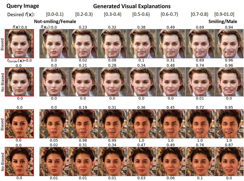
order to detect biases thereby limiting their applicability.     art in terms of the validity, proximity, and sparsity of its ex-
Both of these two methods tend to produce trivial explana-       planations, detecting biases on the datasets, and producing
tions, which only address the attribute that was intended to     multiple explanations for an image. 3) We identify the im-
be classified, without further exploring failure cases due to    portance of finding non-trivial explanations and we propose
biases in the data or spurious correlations. For instance, an    a new benchmark to evaluate how valuable the explanations
explanation that suggests to increase the ‘smile’ attribute      are. 4) We propose to leverage the Fisher information ma-
of a ‘smile’ classifier for an already-smiling face is trivial   trix of the latent space for finding spurious features that pro-
and it does not explain why a misclassification occurred.        duce non-trivial explanations.
On the other hand, a non-trivial explanation that suggests
to change the facial skin color would uncover a racial bias      2. Related Work
in the data that should be addressed by the ML practitioner.
In this work, we focus on diverse valuable explanations,             Explainable artificial intelligence (XAI) is a suite of
that is, valid, proximal, sparse, and non-trivial.               techniques developed to make either the construction or in-
                                                                 terpretation of model decisions more accessible and mean-
    We propose Diverse Valuable Explanations (DiVE), an          ingful. Broadly speaking, there are two branches of work in
explainability method that can interpret ML model predic-        XAI, ad-hoc and post-hoc. Ad-hoc methods focus on mak-
tions by identifying sets of valuable attributes that have the   ing models interpretable, by imbuing model components or
most effect on model output. DiVE produces multiple coun-        parameters with interpretations that are rooted in the data
terfactual explanations which are enforced to be valuable,       themselves [25, 40, 46]. To date, most successful machine
and diverse, resulting in more informative explanations for      learning methods, including deep learning ones, are unin-
machine learning practitioners than competing methods in         terpretable [6, 18, 24, 32].
the literature. Our method first learns a generative model of        Post-hoc methods aim to explain the decisions of un-
the data using a β-TCVAE [5] to obtain a disentangled latent     interpretable models. These methods can be categorized
representation which leads to more proximal and sparse ex-       as non-generative and generative. Non-generative methods
planations. In addition, the VAE is not required to be trained   use information from an ML model to identify the features
on the same dataset as the ML model to be explained. DiVE        most responsible for an outcome for a given input. Ap-
then learns a latent perturbation using constraints to enforce   proaches like [38, 42, 48] interpret ML model decisions by
diversity, sparsity, and proximity. In order to generate non-    fitting a locally interpretable model. Others use the gra-
trivial explanations, DiVE leverages the Fisher information      dient of the ML model parameters to perform feature at-
matrix of its latent space to focus its search on the less in-   tribution [1, 51–53, 55, 61, 62], sometimes by employing
fluential factors of variation of the ML model. This mecha-      a reference distribution for the features [11, 52]. This has
nism enables the discovery of spurious correlations learned      the advantage of identifying alternative feature values that,
by the ML model.                                                 when substituted for the observed values, would result in a
    We provide experiments to assess whether our expla-          different outcome. These methods are limited to small con-
nations are more valuable and diverse than current state-        tiguous regions of features with high influence on the target
of-the-art. First, we assess their validity on the CelebA        model outcome. In so doing, they can struggle to provide
dataset [34] and provide quantitative and qualitative results    plausible changes of the input that are useful for a user in
on a bias detection benchmark [54]. Second, we show that         order to correct a certain output or bias of the model. Gener-
the generated explanations are more proximal in terms of         ative methods such as [4, 5, 7, 15] propose proximal modi-
Fréchet Inception Distance (FID) [20], which is a measure       fications of the input that change the model decision. How-
of similarity between two datasets of images commonly            ever the generated perturbations are usually performed in
used to evaluate the quality of generated images. In addi-       pixel space and bound to masking small regions of the im-
tion, we evaluate the proximity in latent space and face ver-    age without necessarily having a semantic meaning. Closest
ification accuracy, as reported by Singla et al. [54]. Third,    to our work are generative counterfactual explanation meth-
we assess the sparsity of the generated counterfactuals by       ods which synthesize perturbed versions of observed data
computing the average change in facial attributes. Finally,      that result in a change of the model prediction. These can
we propose a new benchmark to quantify the success of ex-        be further subdivided into two families. The first family of
plainability systems at finding non-trivial explanations. We     methods conditions the generative model on attributes, by
find that DiVE is more successful at finding non-trivial ex-     e.g. using a conditional GAN [26, 33, 50, 59, 60]. This
planations than previous methods and baselines.                  dependency on attribute information can restrict the appli-
    We summarize the contributions of this work as follows:      cability of these methods in scenarios where annotations are
1) We propose DiVE, an explainability method that can in-        scarce. Methods in the second family use generative mod-
terpret an ML model by identifying the attributes that have      els such as VAEs [30] or unconditional GANs [14] that do
the most effect on its output. 2) DiVE achieves state of the     not depend on attributes during generation [9, 54]. While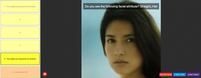
these methods provide valid and proximal explanations for            For training the encoder-decoder architecture we use β-
a model outcome, they fail to provide a diverse set of sparse,   TCVAE [5] since it has been shown to obtain competi-
non-trivial explanations. Mothilal et al. [39] addressed the     tive disentanglement performance [35]. It follows the same
diversity problem by introducing a diversity constraint be-      encoder-decoder structure as the VAE [30], i.e., the input
tween a set of randomly initialized counterfactuals (DICE).      data is first encoded by a neural network qφ (z|x) parame-
However, DICE shares the same problems as [4, 7] since           terized by φ. Then, the input data is recovered by a decoder
perturbations are directly performed on the observed feature     neural network pθ (x|z), parameterized by θ.
space, and it not designed to generate non-trivial explana-          In addition to the β-TCVAE loss, we use the perceptual
tions.                                                           reconstruction loss from Hou et al. [21]. This replaces the
   In this work we propose DiVE, a counterfactual explana-       pixel-wise reconstruction loss by a perceptual reconstruc-
tion method that generates a diverse set of valid, proximal,     tion loss, using the hidden representation of a pre-trained
sparse, and non-trivial explanations. We provide a more          neural network R. Specifically, we learn a decoder Dθ gen-
exhaustive review of the related work in the Appendix.           erating an image, i.e., x̃ = Dθ (z), and this image is re-
                                                                 encoded in a hidden representation: h = R(x̃), and com-
3. Proposed Method                                               pared to the original image in the same space using a nor-
                                                                 mal distribution. Once trained, the weights of the encoder-
    We propose DiVE, an explainability method that can in-
                                                                 decoder are fixed for the rest of the steps of our algorithm.
terpret an ML model by identifying the latent attributes that
have the most effect on its output. Summarized in Figure 1,      3.2. Interpreting the ML model
DiVE uses an encoder, a decoder, and a fixed weight ML
model. The ML model could be any function for which                  In order to find weaknesses in the ML model, DiVE
we have access to its gradients. In this work, we focus on       searches for a collection of n latent perturbations {i }ni=1
a binary image classifier in order to produce visual expla-      such that the decoded output x̃i = Dθ (z + i ) yields a spe-
nations. DiVE consists of two main steps. First, the en-         cific response from the ML model, i.e., f (x̃) = ỹ for any
coder and the decoder are trained in an unsupervised man-        chosen ỹ ∈ [0, 1]. We optimize i ’s by minimizing:
ner to approximate the data distribution on which the ML
                                                                         LDiVE (x, ỹ, {i }ni=1 ) =
                                                                                                       P
model was trained. Unlike PE [54], our encoder-decoder                                                     LCF (x, ỹ, i )
                                                                                                           i
                                                                                                           P
model does not need to train on the same dataset that the                                         +λ·       i Lprox (x, i )
ML model was trained on. Second, we optimize a set of                                             + α · Ldiv ({i }ni=1 ),       (1)
vectors εi to perturb the latent representation z generated
by the trained encoder. The details of the optimization pro-     where λ, and α determine the relative importance of the
cedure are provided in the Appendix. We use the follow-          losses. The minimization is performed with gradient de-
ing 3 main losses for this optimization: a counterfactual        scent and the complete algorithm can be found in the Ap-
loss LCF that attempts to fool the ML model, a proximity         pendix. We now describe the different loss terms.
loss Lprox that constrains the explanations with respect to
the number of changing attributes, and a diversity loss Ldiv
that enforces the explainer to generate diverse explanations     Counterfactual loss. The goal of this loss function is to
with only one confounding factor for each of them. Finally,      identify a change of latent attributes that will cause the ML
we propose several strategies to mask subsets of dimensions      model f to change it’s prediction. For example, in face
in the latent space to prevent the explainer from producing      recognition, if the classifier detects that there is a smile
trivial explanations. Next we explain the methodology in         present whenever the hair is brown, then this loss function
more detail.                                                     is likely to change the hair color attribute. This is achieved
                                                                 by sampling from the decoder x̃ = Dθ (z + ), and optimiz-
3.1. Obtaining meaningful representations.                       ing the binary cross-entropy between the target ỹ and the
    Given a data sample x ∈ X , its corresponding target         prediction f (x̃):
y ∈ {0, 1}, and a potentially biased ML model f (x) that
                                                                  LCF (x, ỹ, ) = ỹ · log(f (x̃)) + (1 − ỹ) · log(1 − f (x̃)). (2)
approximates p(y|x), our method finds a perturbed ver-
sion of the same input x̃ that produces a desired proba-
bilistic outcome ỹ ∈ [0, 1], so that f (x̃) = ỹ. In order      Proximity loss. The goal of this loss function is to con-
to produce semantically meaningful counterfactual expla-         strain the reconstruction produced by the decoder to be sim-
nations, perturbations are performed on a latent representa-     ilar in appearance and attributes as the input. It consists of
tion z ∈ Z ⊆ Rd of the input x. Ideally, each dimension in       the following two terms,
Z represents a different semantic concept of the data, i.e.,
the different dimensions are disentangled.                                   Lprox (x, ) = ||x − x̃||1 + γ · ||||1 ,           (3)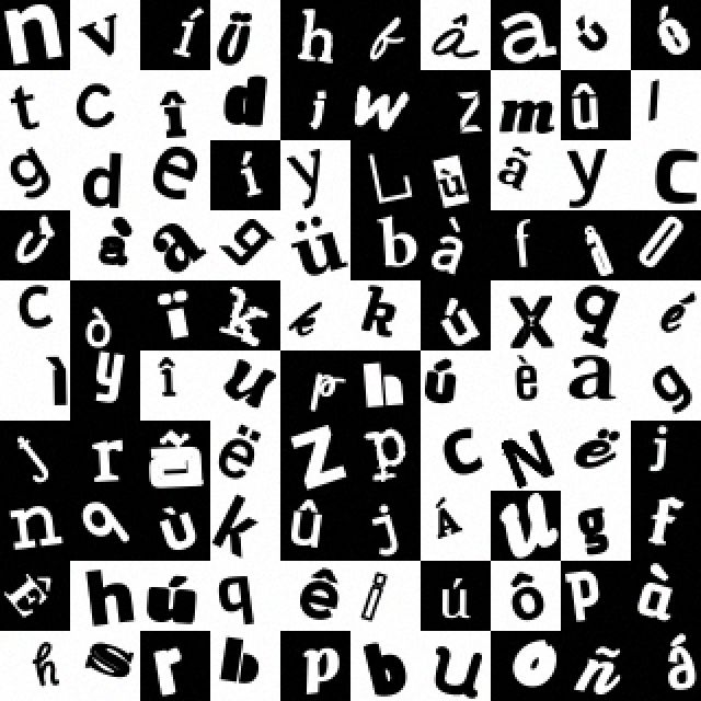
Trivial Counterfactuals
                 Z = Latent representation
                   = Perturbation

                                     Encoder                     Decoder               Not bald       Not bald
                                                                                     Non-Trivial Counterfactuals

                     Bald
                                                                 ML model

                                                                 Not Bald               Not bald      Not bald

Figure 1: DiVE encodes the input image (left) to explain into a latent representation z. Then z is perturbed by  and decoded
as counterfactual examples. During training, LCF finds the set of  that change the ML model classifier outcome while Ldiv
and Lprox enforce that the samples are diverse while staying proximal. These are four valid counterfactuals generated from
the experiment in Section 4.4. However, only the bottom row contains counterfactuals where the man is still bald as indicated
by the oracle or a human. These counterfactuals identify a weakness in the ML model.

where γ is a scalar weighting the relative importance of the      ML model. We estimate the influence of each of the latent
two terms. The first term ensures that the explanations can       factors with the average Fisher information matrix:
be related to the input by constraining the input and the out-
put to be similar. The second term aims to identify a sparse
perturbation to the latent space Z that confounds the ML             F = Ep(i) Eqφ (z|xi ) Ep(y|z) ∇z ln p(y|z) ∇z ln p(y|z)T ,   (5)
model. This constrains the explainer to identify the least
amount of attributes that affect the classifier’s decision in
                                                                    where p(y = 1|z) = f (Dθ (z)), and p(y = 0|z) =
order to produce sparse explanations.
                                                                  1−f (Dθ (z)). The diagonal values of F express the relative
                                                                  influence of each of the latent dimensions on the classifier
Diversity loss. This loss prevents the multiple explana-          output. Since the most influential dimensions are likely to
tions of the model from being identical. For instance, if gen-    be related to the main attribute used by the classifier, we
der and hair color are spuriously correlated with smile, the      propose to prevent Eq. 1 from perturbing them in order to
model should provide images either with different gender or       find more surprising explanations. Thus when producing n
different hair color. To achieve this, we jointly optimize for    explanations, we sort Z by the magnitude of the diagonal,
a collection of n perturbations {i }ni=1 and minimize their      we partition it into n contiguous chunks that will be opti-
pairwise similarity:                                              mized for each of the explanations. We call this method
                             v
                             uX  T                2             DiVEFisher .
                     n
                             u         i    j                       However, DiVEF isher does not guarantee that the dif-
          Ldiv ({i }i=1 ) = t                        .    (4)
                                     ki k2 kj k2                ferent partitions of Z all the factors concerning a trivial
                              i6=j
                                                                  attribute are grouped together. Thus, we propose to parti-
   The method resulting of optimizing Eq. 1 (DiVE) results        tion Z into subsets of latent factors that interact with each
in diverse counterfactuals that are more valid, proximal, and     other when changing the predictions of the ML model. Such
sparse. However, it may still produce trivial explanations,       interaction can be estimated using F as an affinity mea-
such as exaggerating a smile to explain a smile classifier        sure. We use spectral clustering [56] to obtain a partition
without considering other valuable biases in the ML model         of Z. This partition is represented as a collection of masks
such as hair color. While the diversity loss encourages the       {mi }ni=1 , where mi ∈ {0, 1}d represents which dimen-
orthogonality of the explanations, there might still be sev-      sions of Z are part of cluster i. Finally, these masks are
eral latent variables required to represent all variations of     used in Equation 1 to bound each i to its subspace, i.e.,
smile.                                                            0i = i ◦ mi , where ◦ represents element wise multipli-
                                                                  cation. Since these masks are orthogonal, this effectively
Beyond trivial counterfactual explanations. To find               replaces Ldiv . In Section 4, we highlight the benefits of this
non-trivial explanations, we propose to prevent DiVE from         clustering approach by comparing to other baselines. We
perturbing the most influential latent factors of Z on the        call this method DiVEFisherSpectral .
4. Experimental Results
Not-smiling Smiling
: 0.0 : 0.0 0.21 0.28 0.34 0.48 0.74 0.96
In this section, we evaluate the described methods on 5
different aspects: (1) the validity of the generated expla-
PE
nations as well as the ability to discover biases within the
: 0.0 : 0.0 0.0 0.0 0.0 0.0 0.01 0.0
ML model and the data (Section 4.1); (2) their proximity 0.0 0.01 0.18 0.34 0.55 0.66 0.76 1.0
in terms of FID, latent space closeness, and face verifica-
xGEM+
tion accuracy (Section 4.2); (3) the sparsity of the generated
0.0 0.0 0.0 0.0 0.0 0.0 0.0 0.0
counterfactuals (Section 4.3); and (4) the ability to iden- 0.0 0.01 0.25 0.33 0.57 0.67 0.75 0.99
tify diverse non-trivial explanations for image misclassifi-
Ours
cations made by the ML model (Section 4.4); (5) the out-
of-distribution performance of DiVE (Section 4.4). 0.0 0.0
: 0.0
0.0
0.23
0.0
0.32
0.0
0.38
0.0
0.49
0.0
0.69
0.00
0.94
PE
Experimental Setup. To align with [9, 26, 54], we per-
: 0.0 : 0.0 0.02 0.08 0.10 0.31 0.69 0.96
form experiments on the CelebA database [34]. CelebA is 0.0 0.01 0.13 0.32 0.74 0.88 0.95 0.99
a large-scale dataset containing more than 200K celebrity
xGEM+
Biased
facial images. Each image is annotated with 40 binary
0.0 0.0 0.1 0.3 0.5 0.6 0.7 0.99
attributes such as “Smiling”, “Male”, and “Eyeglasses”. 0.0 0.01 0.25 0.32 0.54 0.68 0.80 0.99
These attributes allow us to evaluate counterfactual expla-
nations by determining whether they could highlight spu- Ours
rious correlations between multiple attributes such as “lip- 0.0 0.01 0.27 0.34 0.49 0.57 0.66 0.93
stick” and “smile”. In this setup, explainability methods are
No-Biased
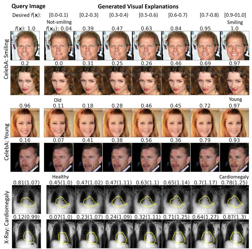
Figure 2: Bias detection experiment. Each column
trained in the training set and ML models are explained on
presents an explanation for a target “Smiling” probability
the validation set. The hyperparameters of the explainer are
interval. Rows contain explanations produced by PE [54],
searched by cross-validation on the training set. We com-
xGEM+ and our DiVE. (a) of a gender-unbiased classi-
pare our method with xGEM [26] and PE [54] as representa-
fier, and (b) corresponds to explanations of a gender-biased
tives of methods that use an unconditional generative model
“Smile” classifier. The classifier output probability is dis-
and a conditional GAN respectively. We use the same train
played on top of the images while the oracle prediction for
and validation splits as PE [54]. DiVE and xGEM do not
gender is displayed at the bottom.
have access to the labeled attributes during training.
We test the out-of-distribution (OOD) performance of
DiVE with the Synbols dataset [31]. Synbols is an image
auto-encoding architecture as DiVE, and PE as described
generator with characters from the Unicode standard and
by Singla et al. [54]. For our methods, we provide imple-
the wide range of artistic fonts provided by the open font
mentation details, architecture description, and algorithm in
community. This provides us to better control on the fea-
the Appendix.
tures present in each set when compared to CelebA. We
generate 100K black and white of 32×32 images from 48
4.1. Validity and bias detection
characters in the latin alphabet and more than 1K fonts. We
use the character type to create disjoint sets for OOD train- We evaluate DiVE’s ability to detect biases in the data.
ing and we use the fonts to introduce biases in the data. We We follow the same procedure as PE [54], and train two bi-
provide a sample of the dataset in the Appendix. nary classifiers for the attribute “Smiling”. The first one is
We compare three version of our method and two ab- trained on a biased version of CelebA where all the male
lated version to three existing methods. DiVE, resulting celebrities are smiling and all the females are not smil-
of optimizing Eq. 1. DiVEFisher , which extends DiVE by ing (fbiased ). This reflects an existing bias in the data
using the Fisher information matrix introduced in Eq. 5. gathering process where female are usually expected to
DiVEFisherSpectral , which extends DiVEFisher with spectral smile [9, 19]. The second one is trained on the unbiased
clustering. We introduce two additional ablations of our version of the data (funbiased ). Both classifiers are eval-
method, DiVE-- and DiVERandom . DiVE-- is equivalent uated on the CelebA validation set. Also following Singla
to DiVE but using a pixel-based reconstruction loss instead et al. [54], we train an oracle classifier (foracle ) based on VG-
of the perceptual loss. DiVERandom uses random masks in- GFace2 [3] which obtains perfect accuracy on the gender
stead of using the Fisher information. Finally, we compare attribute. The hypothesis is that if “Smiling” and “Gender”
our baselines with xGEM as described in Joshi et al. [26], are confounded by the classifier, so should be the explana-
xGEM+, which is the same as xGem but uses the same tions. Therefore, we could identify biases when the gener-ated examples not only change the target attribute but also Table 1: Bias detection experiment. Ratio of generated
the confounded one. To generate the counterfactuals, DiVE counterfactuals classified as “Smiling” and “Non-Smiling”
produces perturbations until it changes the original predic- for a classifier biased on gender (fbiased ) and an unbi-
tion of the classifier, i.e., “Smiling” to “Non-Smiling”. As ased classifier (funbiased ). Bold indicates Overall closest to
described by Singla et al. [54] only valid explanations are Ground truth.
considered, i.e. those that change the original prediction of
the classifier. Target label
We follow the procedure introduced in [26, 54] and re- ML model Smiling Non-Smiling
port a confounding metric for bias detection in Table 1. The model PE xGEM+ DiVE PE xGEM+ DiVE
columns Smiling and Non-Smiling indicate the target class Male 0.52 0.94 0.89 0.18 0.24 0.16
fbiased Female 0.48 0.06 0.11 0.82 0.77 0.84
for counterfactual generation. The rows Male and Female
Overall 0.12 0.29 0.22 0.35 0.33 0.36
contain the proportion of counterfactuals that are classified Ground truth 0.75 0.67
by the oracle as “Male” and “Female”. We can see that
Male 0.48 0.41 0.42 0.47 0.38 0.44
the generated explanations for fbiased are classified more of- funbiased Female 0.52 0.59 0.58 0.53 0.62 0.57
ten as “Male” when the target attribute is “Smiling”, and Overall 0.07 0.13 0.10 0.08 0.15 0.07
“Female” when the target attribute is “Non-Smiling”. The Ground truth 0.04 0.00
confounding metric, denoted as overall, is the fraction of
generated explanations for which the gender was changed
with respect to the original image. It thus reflect the magni- We report these scores in Table 2 for all 3 categories.
tude of the the bias as approximated by the explainers. DiVE produces the best quality counterfactuals, surpassing
Singla et al. [54] consider that a model is better than an- PE by 6.3 FID points for the “Smiling” target and 19.6 FID
other if the confounding metric is the highest on fbiased and points for the “Young” target in the Overall category. DiVE
the lowest on funbiased . However, they assume that fbiased obtains lower FID than xGEM+ which shows that the im-
always predicts the “Gender” based on “Smile”. Instead, provement not only comes from the superior architecture of
we propose to evaluate the confounding metric by compar- our method. Further, there are two other factors that ex-
ing it to the empirical bias of the model, denoted as ground plain the improvement of DiVE’s FID. First, the β-TCVAE
truth in Table 1. Details provided in the Appendix. decomposition of the KL divergence improves the disentan-
We observe that DiVE is more successful than PE at de- glement ability of the model while suffering less reconstruc-
tecting biases although the generative model of DiVE was tion degradation than the VAE. Second, the perceptual loss
not trained with the biased data. While xGEM+ has a higher makes the image quality constructed by DiVE to be compa-
success rate at detecting biases in some cases, it produces rable with that of the GAN used in PE. Additional experi-
lower-quality images that are far from the input. In Figure 2, ments in the Appendix show that DiVE is more successful
we provide samples generated by our method with the two at preserving the identity of the faces than PE and xGEM
classifiers and compare them to PE and xGEM+. We found and thus at producing feasible explanations. These results
that gender changes with the “Smiling” attribute with fbiased suggest that the combination of disentangled latent features
while for funbiased it stayed the same. In addition, we also and the regularization of the latent features help DiVE to
observed that for fbiased the correlation between “Smile” and produce the minimal perturbations of the input that produce
“Gender” is higher than for PE. It can also be observed that a successful counterfactual.
xGEM+ fails to retain the identity of the person in x when In Figure 2 we show qualitative results obtained by tar-
compared to PE and our method. Qualitative results are re- geting different probability ranges for the output of the ML
ported in Figure 2. model as described in PE. DiVE produces more natural-
looking facial expressions than xGEM+ and PE. Additional
4.2. Counterfactual Explanation Proximity results for “Smiling” and “Young” are provided in the Ap-
pendix.
We evaluate the proximity of the counterfactual expla-
nations using FID scores [20] as described by Singla et al.
4.3. Counterfactual Explanation Sparsity
[54]. The scores are based on the target attributes “Smiling”
and “Young”, and are divided into 3 categories: Present, In this section we quantitatively compare the amount of
Absent, and Overall. Present considers explanations for valid and sparse counterfactuals provided by different base-
which the ML model outputs a probability greater than 0.9 lines. Table 3 shows the results for a classifier model trained
for the target attribute. Absent refers to explanations with on the attribute “Young” of the CelebA dataset. The first
a probability lower than 0.1. Overall considers all the suc- row shows the number of attributes that each method change
cessful counterfactuals, which changed the original predic- in average to generate a valid counterfactual. Methods that
tion of the ML model. require to change less attributes are likely to be actionableTable 2: FID of DiVE compared to xGEM [26], Progres- sures a method’s ability to generate valuable explanations.
sive Exaggeration (PE) [54], xGEM trained with our back- For an explanation to be valuable, it should 1) be misclas-
bone (xGEM+), and DiVE trained without the perceptual sified by the ML model (valid), 2) not modify attributes in-
loss (DiVE--) tended to be classified by the ML model (non-trivial), and
3) not have diverged too much from the original sample
Target Attribute xGEM PE xGEM+ DiVE-- DiVE (proximal). A misclassification provides insights into the
Smiling weaknesses of the model. However, the counterfactual is
even more insightful when it stays close to the original im-
Present 111.0 46.9 67.2 54.9 30.6
Absent 112.9 56.3 77.8 62.3 33.6 age as it singles-out spurious correlations learned by the ML
Overall 106.3 35.8 66.9 55.9 29.4 model. Because it is costly to provide human evaluation of
an automatic benchmark, we approximate both the prox-
Young
imity and the real class with the VGGFace2-based oracle.
Present 115.2 67.6 68.3 57.2 31.8 We choose the VGGFace2 model as it is less likely to share
Absent 170.3 74.4 76.1 51.1 45.7 the same biases as the ML model, since it was trained for
Overall 117.9 53.4 59.5 47.7 33.8
a different task than the ML model with an order of mag-
nitude more data. We conduct a human evaluation exper-
Table 3: Average number of attributes changed per ex- iment in the Appendix, and we find a significant correla-
planation and percentage of non-trivial explanations. This tion between the oracle and the human predictions. For 1)
experiment evaluates the counterfactuals generated by dif- and 2) we deem that an explanation is successful if the ML
ferent methods for an ML model trained on the attribute model and the oracle make different predictions about the
“Young” of the CelebA dataset. xGEM++ is xGEM+ using counterfactual. E.g., the top counterfactuals in Figure 1 are
β-TCVAE as generator. not deemed successful explanations because both the ML
model and the oracle agree on its class, however the two in
PE [54] xGEM+ [26] xGEM++ DiVE DiVEFisher DiVEFisherSpectral
the bottom row are successful because only the oracle made
Attr. change 03.74 06.92 06.70 04.81 04.82 04.58
Non-trivial (%) 05.12 18.56 34.62 43.51 42.99 51.07 the correct prediction. These explanations where generated
by DiVEFisherSpectral . As for 3) we measure the proximity
with the cosine distance between the sample and the coun-
by a user. We observe that DiVE changes less attributes on terfactual in the feature space of the oracle.
average than xGEM+. We also observe that DiVEFisherSpectral
We test all methods from Section 4 on a subset of the
is the method that changes less attributes among all the
CelebA validation set described in the Appendix. We re-
baselines. To better understand the effect of disentan-
port the results of the full hyperparameter search. The
gled representations, we also report results for a version of
vertical axis shows the success rate of the explainers, i.e.,
xGEM+ with the β-TCVAE backbone (xGEM++). We do
the ratio of valid explanations that are non-trivial. This
not observe significant effects on the sparsity of the counter-
is the misclassification rate of the ML model on the ex-
factuals. In fact, a fine-grained decomposition of concepts
planations. The dots denote the mean performances and
in the latent space could lead to lower the sparsity.
the curves are computed with Kernel Density Estimation
4.4. Beyond trivial explanations (KDE). On average, DiVE improves the similarity metric
over xGEM+ highlighting the importance of disentangled
Previous works on counterfactual generations tend to representations for identity preservation. Moreover, using
produce trivial input perturbations to change the output of information from the diagonal of the Fisher Information
the ML model. That is, they tend to increase/decrease the Matrix as described in Eq. 5 further improves the expla-
presence of the attribute that is intended to be classified. nations as shown by the higher success rate of DiVEFisher
For instance, in Figure 2 all the explainers put a smile over DiVE and DiVERandom . Thus, preventing the model
on the input face in order to increase the probability for from perturbing the most influential latent factors helps to
“smile”. While that is correct, this explanation does not pro- uncover spurious correlations that affect the ML model. Fi-
vide much insight about the potential weaknesses of the ML nally, the proposed spectral clustering of the full Fisher
model. Instead, in this work we emphasize producing non- Matrix attains the best performance validating that the la-
trivial explanations that are different from the main attribute tent space partition can guide the gradient-based search to-
that the ML model has been trained to identify. These kind wards better explanations. We reach the same conclusions
of explanations provide more insight about the factors that in Table 3, where we provide a comparison with PE for
affect the classifier and thus provide cues on how to improve the attribute “Young”. In addition, we provide results for
the model or how to fix incorrect predictions. a version of xGEM+ with more disentangled latent factors
To evaluate this, we propose a new benchmark that mea- (xGEM++). We find that disentangled representations pro-0.7
xGEM+ 0.70 xGEM+ xGEM+
DiVE DiVERandom 0.8 DiVERandom
0.6
DiVERandom 0.65 DiVE DiVE
0.5 DiVE_Fisher DiVEFisher 0.7 DiVEFisher
DiVE_FisherSpectral 0.60 DiVEFisherSpectral DiVEFisherSpectral
0.4
0.6
success rate
success rate
success rate
0.55
0.3
0.2
0.50 0.5
0.1 0.45
0.4
0.0 0.40
0.1
0.3
0.35
0.75 0.80 0.85 0.90 0.95 0.5 0.6 0.7 0.8 0.9 1.0 0.65 0.70 0.75 0.80 0.85 0.90
embedding similarity (VGG) embedding similarity (Resnet12) embedding similarity (Resnet12)
(a) CelebA (ID) (b) Synbols (ID) (c) Synbols (OOD)
Figure 3: Beyond trivial explanations. The rate of successful explanations (y-axis) plotted against embedding similarity
(x-axis) for all methods. For both metrics, higher is better, i.e., the most valuable explanations are in the top-right corner. For
each method, we ran an hyperparameter sweep and denote the mean of the performances with a dot. The curves are computed
with KDE. The left plot shows the performance on CelebA and the other two plots shows the performance for in-distribution
(ID) and out-of-distribution (OOD) experiments on Synbols. All DiVE methods outperform xGEM+ on both metrics simul-
taneously when conditioning on successful counterfactuals. In both experiments, DiVEFisher and DiVEFisherSpectral improve
the performance over both DiVERandom and DiVE.
vide the explainer with a more precise control on the seman- ily entangled it would fail to produce explanations with a
tic concepts being perturbed, which increases the success sparse amount of features. However, our approach can still
rate of the explainer by 16%. tolerate a small amount of entanglement, yielding a small
decrease in interpretability. We expect that progress in iden-
tifiability [28, 36] will increase the quality of representa-
Out-of-distribution generalization. In the previous ex- tions. With a perfectly disentangled model, our approach
periments, the generative model of DiVE was trained on could still miss some explanations or biases. E.g., with the
the same data distribution (i.e., CelebA faces) as the ML spectral clustering of the Fisher, we group latent variables
model. We test the out-of-distribution performance of DiVE and only produce a single explanation per group in order
by training its auto-encoder on a subset of the latin alphabet to present explanations that are conceptually different. This
of the Synbols dataset [31]. Then, counterfactual explana- may leave behind some important explanations, but the user
tions are produced for a different disjoint subset of the al- can simply increase the number of clusters or the number of
phabet. To evaluate the effectiveness of DiVE in finding bi- explanations per clusters for a more in-depth analysis.
ases on the ML model, we introduce spurious correlations
in the data. Concretely, we assign a different set of fonts In addition to the challenge of achieving disentangled
to each of the letters in the alphabet as detailed in the Ap- representations, finding the optimal hyperparameters for the
pendix. In-distribution (ID) results are reported in Figure 3b VAE and their generalization out of the training distribution
for reference, and OD results are reported in Figure 3c. We is an open problem. Moreover, if the generative model is
observe that DiVE is able to find valuable countefactuals trained on biased data, one could expect the counterfactuals
even when the VAE was not trained on the same data dis- to be biased as well. However, as we show in Figure 3c, our
tribution. Moreover, results are consistent with the CelebA model still finds non-trivial explanations when applied out
experiment, with DiVE outperforming xGEM+ and Fisher of distribution. In that way, it could be trained on a larger
information-based methods outperforming the rest. unlabeled dataset to overcome possible biases caused by the
lack of annotated data.
5. Limitations and Future Work Although the generative model plays an important role
to produce valuable counterfactuals in the computer vision
This work shows that a good generative model can pro- domain, our work could be extended to other domains. For
vide interesting insights on the biases of an ML model. example, Eq. 1 could be applied to find non-trivial expla-
However, this relies on a properly disentangled representa- nations on tabular data by directly optimizing the observed
tion. In the case where the generative model would be heav- features instead of the latent factors of the VAE. However,further work would be needed to adapt the DiVE loss func- for black box decision making. IEEE Intelligent Systems, 34
tions to produce perturbations on discrete and categorical (6):14–23, 2019. 16
variables. [17] R. Guidotti, A. Monreale, S. Matwin, and D. Pedreschi.
Black box explanation by learning image exemplars in the la-
tent feature space. In Joint European Conference on Machine
References Learning and Knowledge Discovery in Databases, pages
[1] J. Adebayo, J. Gilmer, M. Muelly, I. Goodfellow, M. Hardt, 189–205. Springer, 2019. 16
and B. Kim. Sanity checks for saliency maps. In Advances [18] K. He, X. Zhang, S. Ren, and J. Sun. Deep residual learn-
in Neural Information Processing Systems, 2018. 2, 17 ing for image recognition. In Computer Vision and Pattern
[2] A. Brock, J. Donahue, and K. Simonyan. Large scale gan Recognition, 2016. 2
training for high fidelity natural image synthesis. arXiv [19] D. Hestenes and I. Halloun. Interpreting the force concept
preprint arXiv:1809.11096, 2018. 12 inventory: A response to march 1995 critique by huffman
[3] Q. Cao, L. Shen, W. Xie, O. M. Parkhi, and A. Zisserman. and heller. The physics teacher, 33(8):502–502, 1995. 5
Vggface2: A dataset for recognising faces across pose and [20] M. Heusel, H. Ramsauer, T. Unterthiner, B. Nessler, and
age. In International Conference on Automatic Face and S. Hochreiter. Gans trained by a two time-scale update rule
Gesture Recognition, 2018. 5, 12 converge to a local nash equilibrium. In Advances in Neural
[4] C.-H. Chang, E. Creager, A. Goldenberg, and D. Duvenaud. Information Processing Systems, 2017. 2, 6
Explaining image classifiers by counterfactual generation. [21] X. Hou, L. Shen, K. Sun, and G. Qiu. Deep feature consis-
In International Conference on Learning Representations, tent variational autoencoder. In Winter Conference on Appli-
2019. 1, 2, 3, 17 cations of Computer Vision, 2017. 3
[5] R. T. Chen, X. Li, R. B. Grosse, and D. K. Duvenaud. [22] G. Huang, Z. Liu, L. Van Der Maaten, and K. Q. Weinberger.
Isolating sources of disentanglement in variational autoen- Densely connected convolutional networks. In Computer Vi-
coders. In Advances in Neural Information Processing Sys- sion and Pattern recognition, 2017. 12
tems, 2018. 2, 3, 17 [23] S. Ioffe and C. Szegedy. Batch normalization: Accelerating
[6] C. Cortes and V. Vapnik. Support-vector networks. Machine deep network training by reducing internal covariate shift. In
learning, 20(3):273–297, 1995. 2 International Conference on Machine Learning, 2015. 12
[7] P. Dabkowski and Y. Gal. Real time image saliency for black [24] S. Jégou, M. Drozdzal, D. Vazquez, A. Romero, and Y. Ben-
box classifiers. arXiv preprint arXiv:1705.07857, 2017. 2, gio. The one hundred layers tiramisu: Fully convolutional
3, 17 densenets for semantic segmentation. In Computer Vision
[8] J. Deng, W. Dong, R. Socher, L.-J. Li, K. Li, and L. Fei- and Pattern Recognition Workshops, 2017. 2
Fei. Imagenet: A large-scale hierarchical image database. In [25] F. V. Jensen et al. An introduction to Bayesian networks,
Computer Vision and Pattern Recognition, 2009. 12 volume 210. UCL press London, 1996. 2
[9] E. Denton, B. Hutchinson, M. Mitchell, and T. Gebru. De- [26] S. Joshi, O. Koyejo, B. Kim, and J. Ghosh. xgems: Gener-
tecting bias with generative counterfactual face attribute aug- ating examplars to explain black-box models. arXiv preprint
mentation. arXiv preprint arXiv:1906.06439, 2019. 2, 5, 17 arXiv:1806.08867, 2018. 1, 2, 5, 6, 7, 11, 13, 15, 17
[10] A. Dhurandhar, P.-Y. Chen, R. Luss, C.-C. Tu, P. Ting, [27] A.-H. Karimi, G. Barthe, B. Balle, and I. Valera. Model-
K. Shanmugam, and P. Das. Explanations based on the miss- agnostic counterfactual explanations for consequential deci-
ing: Towards contrastive explanations with pertinent nega- sions. In International Conference on Artificial Intelligence
tives. In Advances in Neural Information Processing Sys- and Statistics, pages 895–905, 2020. 16
tems, pages 592–603, 2018. 17 [28] I. Khemakhem, D. Kingma, R. Monti, and A. Hyvari-
[11] R. C. Fong and A. Vedaldi. Interpretable explanations of nen. Variational autoencoders and nonlinear ica: A unifying
black boxes by meaningful perturbation. In International framework. In International Conference on Artificial Intelli-
Conference on Computer Vision, 2017. 1, 2, 17 gence and Statistics, pages 2207–2217. PMLR, 2020. 8
[12] H. Fu, C. Li, X. Liu, J. Gao, A. Celikyilmaz, and L. Carin. [29] D. P. Kingma and J. Ba. Adam: A method for stochastic
Cyclical annealing schedule: A simple approach to mitigat- optimization. arXiv preprint arXiv:1412.6980, 2014. 12
ing kl vanishing. arXiv preprint arXiv:1903.10145, 2019. [30] D. P. Kingma and M. Welling. Auto-encoding variational
12 bayes. arXiv preprint arXiv:1312.6114, 2013. 2, 3
[13] Y. Gal, J. Hron, and A. Kendall. Concrete dropout. In Ad- [31] A. Lacoste, P. Rodrı́guez López, F. Branchaud-Charron,
vances in neural information processing systems, 2017. 1 P. Atighehchian, M. Caccia, I. H. Laradji, A. Drouin,
[14] I. Goodfellow, J. Pouget-Abadie, M. Mirza, B. Xu, M. Craddock, L. Charlin, and D. Vázquez. Synbols: Prob-
D. Warde-Farley, S. Ozair, A. Courville, and Y. Bengio. Gen- ing learning algorithms with synthetic datasets. Advances in
erative adversarial nets. In Advances in Neural Information Neural Information Processing Systems, 33, 2020. 5, 8, 14
Processing Systems, 2014. 2, 17 [32] Y. LeCun, B. Boser, J. S. Denker, D. Henderson, R. E.
[15] Y. Goyal, Z. Wu, J. Ernst, D. Batra, D. Parikh, and Howard, W. Hubbard, and L. D. Jackel. Backpropagation
S. Lee. Counterfactual visual explanations. arXiv preprint applied to handwritten zip code recognition. Neural Compu-
arXiv:1904.07451, 2019. 2, 17 tation, 1(4):541–551, 1989. 2
[16] R. Guidotti, A. Monreale, F. Giannotti, D. Pedreschi, S. Rug- [33] S. Liu, B. Kailkhura, D. Loveland, and Y. Han. Generative
gieri, and F. Turini. Factual and counterfactual explanations counterfactual introspection for explainable deep learning. In2019 IEEE Global Conference on Signal and Information arXiv preprint arXiv:2101.06046, 2021. 2
Processing (GlobalSIP), pages 1–5. IEEE, 2019. 2 [51] R. R. Selvaraju, M. Cogswell, A. Das, R. Vedantam,
[34] Z. Liu, P. Luo, X. Wang, and X. Tang. Deep learning face D. Parikh, and D. Batra. Grad-cam: Visual explanations
attributes in the wild. In International Conference on Com- from deep networks via gradient-based localization. In In-
puter Vision, 2015. 2, 5 ternational Conference on Computer Vision, 2017. 1, 2, 17
[35] F. Locatello, S. Bauer, M. Lucic, G. Raetsch, S. Gelly, [52] A. Shrikumar, P. Greenside, and A. Kundaje. Learning im-
B. Schölkopf, and O. Bachem. Challenging common as- portant features through propagating activation differences.
sumptions in the unsupervised learning of disentangled rep- arXiv preprint arXiv:1704.02685, 2017. 1, 2, 17
resentations. In International Conference on Machine Learn- [53] K. Simonyan, A. Vedaldi, and A. Zisserman. Deep inside
ing, 2019. 3 convolutional networks: Visualising image classification
[36] F. Locatello, B. Poole, G. Rätsch, B. Schölkopf, O. Bachem, models and saliency maps. arXiv preprint arXiv:1312.6034,
and M. Tschannen. Weakly-supervised disentanglement 2013. 2, 17
without compromises. arXiv preprint arXiv:2002.02886, [54] S. Singla, B. Pollack, J. Chen, and K. Batmanghelich. Ex-
2020. 8 planation by progressive exaggeration. In International Con-
[37] J. Lucas, G. Tucker, R. Grosse, and M. Norouzi. Understand- ference on Learning Representations, 2020. 1, 2, 3, 5, 6, 7,
ing posterior collapse in generative latent variable models. 11, 12, 15, 16
2019. 12 [55] J. T. Springenberg, A. Dosovitskiy, T. Brox, and M. Ried-
[38] S. M. Lundberg and S.-I. Lee. A unified approach to inter- miller. Striving for simplicity: The all convolutional net.
preting model predictions. In Advances in neural informa- arXiv preprint arXiv:1412.6806, 2014. 2, 17
tion processing systems, 2017. 1, 2, 16 [56] X. Y. Stella and J. Shi. Multiclass spectral clustering. In null,
[39] R. K. Mothilal, A. Sharma, and C. Tan. Explaining machine page 313. IEEE, 2003. 4
learning classifiers through diverse counterfactual explana- [57] D. Ulyanov, A. Vedaldi, and V. Lempitsky. Instance normal-
tions. In Conference on Fairness, Accountability, and Trans- ization: The missing ingredient for fast stylization. arXiv
parency, 2020. 1, 3, 17 preprint arXiv:1607.08022, 2016. 12
[40] J. A. Nelder and R. W. Wedderburn. Generalized linear mod- [58] A. Van Looveren and J. Klaise. Interpretable counterfac-
els. Journal of the Royal Statistical Society: Series A (Gen- tual explanations guided by prototypes. arXiv preprint
eral), 135(3):370–384, 1972. 2 arXiv:1907.02584, 2019. 17
[41] B. Oreshkin, P. Rodrı́guez López, and A. Lacoste. Tadam: [59] A. Van Looveren, J. Klaise, G. Vacanti, and O. Cobb. Con-
Task dependent adaptive metric for improved few-shot learn- ditional generative models for counterfactual explanations.
ing. Advances in Neural Information Processing Systems, arXiv preprint arXiv:2101.10123, 2021. 2
31:721–731, 2018. 15 [60] F. Yang, N. Liu, M. Du, and X. Hu. Generative counterfactu-
[42] N. Papernot and P. McDaniel. Deep k-nearest neighbors: als for neural networks via attribute-informed perturbation.
Towards confident, interpretable and robust deep learning. arXiv preprint arXiv:2101.06930, 2021. 2
arXiv preprint arXiv:1803.04765, 2018. 2 [61] B. Zhou, A. Khosla, A. Lapedriza, A. Oliva, and A. Torralba.
[43] M. Pawelczyk, K. Broelemann, and G. Kasneci. Learning Object detectors emerge in deep scene cnns. arXiv preprint
model-agnostic counterfactual explanations for tabular data. arXiv:1412.6856, 2014. 2, 17
In Proceedings of The Web Conference 2020, pages 3126– [62] B. Zhou, A. Khosla, A. Lapedriza, A. Oliva, and A. Tor-
3132, 2020. 17 ralba. Learning deep features for discriminative localization.
[44] E. Perez, F. Strub, H. De Vries, V. Dumoulin, and In Computer Vision and Pattern Recognition, 2016. 2, 17
A. Courville. Film: Visual reasoning with a general con-
ditioning layer. arXiv preprint arXiv:1709.07871, 2017. 12
[45] R. Poyiadzi, K. Sokol, R. Santos-Rodriguez, T. De Bie, and
P. Flach. Face: feasible and actionable counterfactual expla-
nations. In Proceedings of the AAAI/ACM Conference on AI,
Ethics, and Society, pages 344–350, 2020. 17
[46] J. R. Quinlan. Induction of decision trees. Machine Learn-
ing, 1:81–106, 1986. 2
[47] P. Ramachandran, B. Zoph, and Q. V. Le. Searching for acti-
vation functions. International Conference on Learning Rep-
resentations, 2018. 12
[48] M. T. Ribeiro, S. Singh, and C. Guestrin. ”why should i
trust you?” explaining the predictions of any classifier. In
International Conference on Knowledge Discovery and Data
Mining, 2016. 1, 2, 16
[49] C. Russell. Efficient search for diverse coherent explana-
tions. In Conference on Fairness, Accountability, and Trans-
parency, 2019. 1
[50] A. Sauer and A. Geiger. Counterfactual generative networks.Query Image Generated Visual Explanations
Appendix Desired [0-0.1) [0.2-0.3) [0.3-0.4) [0.5-0.6) [0.6-0.7) [0.7-0.8) [0.9-1.0)
Old Young
0.96 0.11 0.18 0.28 0.46 0.45 0.75 0.97
Section A shows additional qualitative results, Section B
contains additional results for identity preservation, Sec-
PE
tion C contains the implementation details, Section D con-
0.96 0.25 0.25 0.34 0.55 0.65 0.75 0.95
tains additional information about the experimental setup,
XGEM+
Section E provides the results of human evaluation of DiVE,
Section F contains details about the model architecture, 0.96 0.03 0.2 0.3 0.5 0.6 0.7 0.96
Section G contains the DiVE Algorithm, Section H contains
Ours
details about the OOD experiment, and Section J contains
the extended related work. 0.16 0.07 0.41 0.38 0.56 0.36 0.79 0.93
PE
A. Qualitative results
0.16 0.07 0.21 0.3 0.5 0.6 0.7 0.96
XGEM+
Figure 4,5 present counterfactual explanations for addi-
tional persons and attributes. The results show that DiVE
achieves higher quality reconstructions compared to other 0.16 0.07 0.21 0.3 0.5 0.6 0.7 0.96
methods. Further, the reconstructions made by DiVE are
Ours
more correlated with the desired target for the ML model
output f (x). We compare DiVE to PE and xGEM+. We
found that gender changes with the “Smiling” attribute with Figure 5: Qualitative results of DiVE, Progressive Exag-
fbiased while for funbiased it stayed the same. In addition, geration (PE) [54], and xGEM+ for the “Young” attribute.
we also observed that for fbiased the correlation between Each column shows the explanations generated for a target
“Smile” and “Gender” is higher than for PE. It can also be probability output of the ML model. The numbers on top of
observed that xGEM+ fails to retain the identity of the per- each row show the actual output of the ML model.
son in x when compared to PE and our method. Finally,
Figure 6 shows successful counterfactuals for different in-
stantiations of DiVE.
DiVE w/o
Query Image Generated Visual Explanations
Desired [0-0.1) [0.2-0.3) [0.3-0.4) [0.5-0.6) [0.6-0.7) [0.7-0.8) [0.9-1.0)
Not-smiling Smiling
: 1.0 : 0.04 0.39 0.47 0.63 0.84 0.95 1.0 original
DiVE
PE
DiVE w/o
1.0 0.01 0.25 0.35 0.55 0.65 0.75 0.97
DiVE-F
XGEM+
DiVE
1.0 0.0 0.25 0.35 0.55 0.66 0.76 0.99
DiVE-FS
Ours
DiVE-F
0.2 0.0 0.31 0.25 0.26 0.46 0.69 0.97
Figure 6: Successful counterfactual generations for differ-
PE
DiVE-FS
ent instantiations of DiVE. Here, the original image was
0.2 0.0 0.26 0.35 0.55 0.65 0.76 0.99
misclassified as non-smiling. All methodologies were able
XGEM+
to correctly add a smile to the woman.
0.2 0.0 0.25 0.35 0.54 0.66 0.74 0.96
Ours
Note that PE directly optimizes the generative model to
take an input variable δ ∈ R that defines the desired output
probability ỹ = f (x) + δ. To obtain explanations at dif-
Figure 4: Qualitative results of DiVE, Progressive Exagger- ferent probability targets, we train a second order spline on
ation (PE) [54], and xGEM [26] for the “Smiling” attribute. the trajectory of perturbations produced during the gradient
Each column shows the explanations generated for a target descent steps of our method. Thus, given the set of perturba-
probability output of the ML model. The numbers on top of tions {εt }, ∀t ∈ 1..τ , obtained during τ gradient steps, and
each row show the actual output of the ML model. the corresponding black-box outputs {f (y|εt )}, the spline
obtains the εỹ for a target output ỹ by interpolation.
0.96 0.03 0.2 0.3 0.5 0.6 0.7 0.96CelebA:Smiling CelebA:Young
xGEM PE xGEM+ DiVE (ours) xGEM PE xGEM+ DiVE (ours)
Latent Space Closeness 88.2 88.0 99.8 98.7 89.5 81.6 97.5 99.1
Face Verification Accuracy 0.0 85.3 91.2 97.3 0.0 72.2 97.4 98.2
Table 4: Identity preserving performance on two prediction tasks.
B. Identity preservation the posterior equal to the prior for these extra dimensions.
More can be found on the topic in [37]. In practice, we ex-
As argued, valuable explanations should remain proxi- perimented with d = {64, 128, 256} and found that with
mal to the original image. Accordingly, performed the iden- d = 128 we achieved a slightly lower ELBO.
tity preservation experiment found in [54] to benchmark To project the 2d features produced by the encoder to a
the methodologies against each other. Specifically, use the flat vector (µ, log (σ 2 )), and to project the sampled codes
VGGFace2-based [3] oracle to extract latent codes for the z to a 2d space for the decoder, we use 3-layer MLPs. For
original images as well as for the explanations and report the face attribute classifiers, we use the same DenseNet [22]
latent space closeness as the fraction of time the explana- architecture as described in Progressive Exaggeration [54].
tions’ latent codes are the closest to their respective original
image latent codes’ compared to the explanations on dif-
Optimization details. All the models are optimized with
ferent original images. Further, we report face verification
Adam [29] with a batch size of 256. During the training
accuracy which consist of the fraction of time the cosine
step, the auto-encoders are optimized for 400 epochs with
distance between the aforementioned latent codes is below
a learning rate of 4 · 10−4 . The classifiers are optimized
0.5.
for 100 epochs with a learning rate of 10−4 . To prevent the
Table 4 presents both metrics for DiVE and its baselines
auto-encoders from suffering KL vanishing, we adopt the
on the “Smilling” and “Young” classification tasks. We find
cyclical annealing schedule proposed by Fu et al. [12].
that DiVE outperforms all other methods on the “Young”
classification task and almost all on the ”Smiling” task.
Counterfactual inference details. At inference time, the
perturbations are optimized with Adam until the ML model
C. Implementation details
output for the generated explanation f (x̃) only differs from
In this Section, we provide provide the details to ensure the target output ỹ by a margin δ or when a maximum num-
the that our method is reproducible. ber of iterations τ is reached. We set τ = 20 for all the
experiments since more than 90% of the counterfactuals are
found after that many iterations. The different i are initial-
Architecture details. DiVE’s architecture is a variation
ized by sampling from a normal distribution N ∼ (0, 0.01).
BigGAN [2] as shown in Table 6. We chose this archi-
For the DiVEF isher baseline, to identify the most valuable
tecture because it achieved impressive FID results on the
explanations, we sort by the magnitude of f = diag(F ).
ImageNet [8]. The decoder (Table 6b) is a simplified ver-
Then, we divide the dimensions of the sorted into N con-
sion of the 128 × 128 BigGAN’s residual generator, without D
tiguous partitions of size k = N , where D is the dimen-
non-local blocks nor feature concatenation. We use Instan-
ceNorm [57] instead of BatchNorm [23] to obtain consistent sionality of Z. Formally, let be sorted by f , then (f )
(f )
outputs at inference time without the need of an additional is constrained as follows,
(
mechanism such as recomputing statistics [2]. All the In- (f ) 0, if j ∈ [(i − 1) · k, i · k]
stanceNorm operations of the decoder are conditioned on εi,j = (f ) , (6)
εi,j , otherwise
the input code z in the same way as FILM layers [44]. The
encoder (Table 6a) follows the same structure as the Big- where i ∈ 1..N indexes each of the multiple ε, and j ∈
GAN 128×128 discriminator with the same simplifications 1..D indexes the dimensions of ε. As a result we obtain
done to our generator. We use the Swish non-linearity [47] partitions with different order of complexity. Masking the
in all layers except for the output of the decoder, which uses first partition results in explanations that are most implicit
a Tanh activation. within the model and the data. On the other hand, mask-
For all experiments we use a latent feature space of 128 ing the last partition results in explanations that are more
dimensions. The ELBO has a natural principled way of se- explicit.
lecting the dimensionality of the latent representation. If To compare with Singla et al. [54] in Figures 4-5 we pro-
d is larger than necessary, it will not enhance the recon- duced counterfactuals at arbitrary target values ỹ of the out-
struction error and the optimization of the ELBO will make put of the ML model classifier. One way to achieve thisYou can also read