Bayesian Nonparametric Learning for Point Processes with Spatial Homogeneity: A Spatial Analysis of NBA Shot Locations
←
→
Page content transcription
If your browser does not render page correctly, please read the page content below
Bayesian Nonparametric Learning for Point Processes with Spatial
              Homogeneity: A Spatial Analysis of NBA Shot Locations

                                     Fan Yin 1 Jieying Jiao 2 Jun Yan 2 Guanyu Hu 3

                         Abstract                                  shed light on the evolution of defensive tactics, which has
                                                                   aroused substantial research interests from the statistical
      Basketball shot location data provide valu-                  community (e.g., Reich et al., 2006; Miller et al., 2014;
      able summary information regarding players to                Franks et al., 2015; Cervone et al., 2016; Jiao et al., 2021a;
      coaches, sports analysts, fans, statisticians, as            Hu et al., 2020b). As shot location data are naturally rep-
      well as players themselves. Represented by spa-              resented by spatial points, developments of novel methods
      tial points, such data are naturally analyzed with           for analyzing spatial point patterns are of fundamental im-
      spatial point process models. We present a novel             portance.
      nonparametric Bayesian method for learning the
      underlying intensity surface built upon a com-               The literature on spatial point pattern data is voluminous
      bination of Dirichlet process and Markov ran-                (see, e.g., Illian et al., 2008; Diggle, 2013; Guan, 2006;
      dom field. Our method has the advantage of                   Guan & Shen, 2010; Baddeley, 2017; Jiao et al., 2021b).
      effectively encouraging local spatial homogene-              The most frequently adopted class of models in empirical
      ity when estimating a globally heterogeneous in-             research is nonhomogeneous Poisson processes (NHPP),
      tensity surface. Posterior inferences are per-               or more generally, Cox processes, including log-Gaussian
      formed with an efficient Markov chain Monte                  Cox process (Møller et al., 1998). Such parametric mod-
      Carlo (MCMC) algorithm. Simulation studies                   els impose restrictions on the functional forms of under-
      show that the inferences are accurate and the                lying process intensity, which can suffer from underfitting
      method is superior compared to a wide range of               of data when there is a misfit between the complexity of
      competing methods. Application to the shot lo-               the model and the data available. In contrast, nonparamet-
      cation data of 20 representative NBA players in              ric approaches such as two-way kernel density estimation
      the 2017-2018 regular season offers interesting              provide more flexibility compared to parametric modeling
      insights about the shooting patterns of these play-          as the underfitting can be mitigated by using models with
      ers. A comparison against the competing method               unbounded complexity.
      shows that the proposed method can effectively               Several important features of the shot location data need to
      incorporate spatial contiguity into the estimation           be captured in any realistic nonparametric method. First,
      of intensity surfaces.                                       near regions are highly likely to have similar intensities.
                                                                   This makes that certain spatial contiguous constraints on
                                                                   the intensity surface desirable. Existing method such as
1. Introduction                                                    mixture of finite mixtures (MFM) of nonhomogeneous
                                                                   Poisson processes (Taddy & Kottas, 2012; Geng et al.,
Quantitative analytics have been a key driving force for ad-
                                                                   2021) is lacking in this aspect. There are also rich litera-
vancing modern professional sports, and there is no excep-
                                                                   ture (Blei & Frazier, 2011; Müller et al., 2011; Ghosh et al.,
tion for professional basketball (Kubatko et al., 2007). In
                                                                   2011; Page et al., 2016; Dahl et al., 2017) discussing spa-
professional basketball, analyses of shooting patterns of-
                                                                   tial constraint prior for regression models however lacking
fer important insights about players’ attacking styles and
                                                                   the discussion on intensity estimation of spatial point pat-
  *
    Equal contribution 1 Department of Statistics, University of   tern data. Second, spatial contiguous constraints should not
California, Irvine, CA, USA 2 Department of Statistics, Univer-    dominate the intensity surface globally (Hu et al., 2020a;
sity of Connecticut, Storrs, CT, USA 3 Department of Statistics,   Zhao et al., 2020). For some players, there are more than
University of Missouri, Columbia, MO, USA. Correspondence          one hot zones in their one-season shooting. Some play-
to: Guanyu Hu .
                                                                   ers will prefer more corner three and top three rather than
Proceedings of the 39 th International Conference on Machine       45 degrees. Although, the corner is not spatial contigu-
Learning, Baltimore, Maryland, USA, PMLR 162, 2022. Copy-          ous with top area, the same intensity value can still belong
right 2022 by the author(s).
Bayesian Nonparametric Learning for Point Processes
to spatially disconnected regions that are sufficiently sim- B, and it is synonymous with complete spatial randomness
ilar with respect to intensity values, which is not well ac- (CSR).
commodated by the penalized method (Li & Sang, 2019).
From the application prospect, zone defense is common de- 2.2. Nonparametric Bayesian Methods for NHPP
fense strategy in NBA from 2001. In addition, each play-
ers will have floor coverage in court. Knowing the hot re- As the CSR assumption over the entire study region rarely
gions rather than small hot points will help the team opti- holds in real-world problems, and to simplify the poten-
mize their team defense strategy. For some players, there tially overcomplicated problem induced by complete non-
are more than one hot zones in their one-season shooting. homogeneity on intensity values, Teng et al. (2017) pro-
Finally, the extent to which the spatial contiguous affects posed to approximate the intensity function λ(s) by a
the intensity surface may differ from player to player, and piecewise constant function. Specifically, the study re-
needs to be learned from the data. gion B is partitioned into n disjoint regions and the in-
tensity over each region is assumed to be constant. Let
To address these challenges, we consider a spatially con- A1 , A2 , . . . , An be a partition of B, i.e., ∪ni=1 Ai = B and
strained Bayesian nonparametric method for point pro- Ai ∩ Aj = ∅, ∀i ̸= j. For each region Ai , i = 1, . . . , n, we
cesses to capture the spatial homogeneity of intensity sur- have λ(s) = λi , ∀ s ∈ Ai . Therefore, the likelihood (2.1)
faces. Our contributions are three-fold. First, we develop a can be written as
novel nonparametric Bayesian method for intensity estima- n
tion of spatial point processes. Compared to existing meth-
Y
fpoisson (NY (Ai )|λi µ(Ai )), (2.2)
ods, the proposed approach is capable of capturing both i=1
locally spatially contiguous clusters and globally discon- R
tinuous clusters and the number of clusters. Second, an where µ(Ai ) = Ai 1ds is the area of region Ai and
efficient Markov chain Monte Carlo (MCMC) algorithm fpoisson (·|λ) is the probability mass function of the Poisson
is designed for our model without complicated reversible distribution with rate parameter λ. For ease of notation, we
jump MCMC. Lastly, we gain important insights about the use N (Ai ) for NY (Ai ) throughout the remainder of the
shooting behaviors of NBA players based on an application text.
to their shot location data. The heterogeneity in the intensity function across different
regions can be naturally represented through a latent clus-
2. Model Specification tering structure. The conventional finite mixture modeling
framework (McLachlan & Basford, 1988; Bouveyron et al.,
2.1. NHPP 2019) assumes that the heterogeneity can be characterized
Spatial point process models provide a natural framework by a discrete set of subpopulations or clusters, such that the
for capturing the random behavior of event location data. points located in the regions belonging to any given sub-
Let S = {s1 , . . . , sN } with si = (xi , yi ), be the set of population tend to be produced by similar intensities. The
observed locations in a pre-defined, bounded region B ⊆ selection of the number of clusters (or components) in fi-
R2 . Let the underlying stochastic mechanism that gives nite mixture models are often recasted as statistical model
rise to the observed point pattern S be P denoted as spatial selection problems which can solved using information cri-
i=1 1(si ∈ A)
N teria (Fraley & Raftery, 2002) or cross-validation (Fu &
point process Y. Process NY (A) =
is a counting process associated with Y, which counts the Perry, 2020), among others. Despite its prevalence in em-
number of points falling into area A ⊆ B. pirical research, such model selection procedures for finite
mixture model ignore uncertainty in the number of clusters,
The NHPP model assumes conditionally independent event which may in turn lead to increased erroneous cluster as-
locations given the process intensity λ(s). For an NHPP, signments. The Bayesian nonparametric approach provides
the number of events in area A, NY (A),R follows Poisson an alternative to parametric modeling and model selection.
distribution with rate parameter λ(A) = A λ(s)ds. In ad- The Dirichlet process (Ferguson, 1973) is currently one of
dition, NY (A1 ) and NY (A2 ) are independent if two areas the most popular Bayesian nonparametric models and it can
A1 ⊆ B and A2 ⊆ B are disjoint. Given the observed point be viewed as the limit of the following finite mixture model
pattern S on fixed region B, the likelihood of the NHPP
model is QN
i=1 λ(si ) yi |Zi , βZi ∼ F (βZi )
R , (2.1)
exp( B λ(s)ds) Zi |p ∼ Discrete(p1 , · · · , pK ) (2.3)
where λ(si ) is the intensity function evaluated at location βZi ∼ G0 p ∼ DirichletK (α/K, · · · , α/K)
si . The NHPP reduces to a homogeneous Poisson process
(HPP) when λ(s) is constant over the entire study region where Zi stands for the cluster of ith observation, βciBayesian Nonparametric Learning for Point Processes
means the parameter of ci th cluster, α stands for the pre- To mitigate the inconsistency in estimating the number of
cision parameter, and G0 is the base measure in Dirichlet clusters caused by CRP, Miller & Harrison (2018) proposed
process, which is also the prior on cluster specific param- to modify CRP with the Mixture of finite mixtures (MFM)
eters β’s. As K → ∞, the model becomes a Dirichlet model. An alternative model which will be used as a bench-
process mixture (DPM) model Neal (2000), which can be mark for comparison is the MFM of NHPP (MFM-NHPP)
used to simultaneously estimate the number of clusters and (Geng et al., 2021).
cluster configurations. Combining DPM with NHPP yields
the following DPM-NHPP model 2.3. Incorporating Spatial Homogeneity
Spatial events typically obey the so-called first law of
N (Ai ) | λ1 , . . . , λn ∼ P oisson(λi µ(Ai )) i = 1, . . . , n, geography, “everything is related to everything else, but
n
near things are more related than distant things” (Tobler,
(λ1 , . . . , λn ) ∼
Y
G(λi ) 1970). This means spatial smoothness, also known as spa-
i=1
tial homogeneity. To incorporate such spatial homogene-
ity, we impose a Markov random field constraint (Besag
G ∼ DP(α, G0 )
et al., 1995; Orbanz & Buhmann, 2008) M (λ1 , . . . , λn ) :=
(2.4) 1
ZH exp {−H(λ1 , . . . , λn )} on λ to encourage the inten-
sity parameters in nearby regions to be similar
where the Dirichlet process (DP) here is parameterized by
a base measure G0 ≡ Gamma(a, b) and a concentration
parameter α. Given λ1 , . . . , λn drawn from G, a condi- G ∼ DP(α, G0 )
tional prior can be obtained by integration (Blackwell & n
MacQueen, 1973)
Y
(λ1 , . . . , λn ) ∼ M (λ1 , . . . , λn ) G(λi )
i=1
n N (Ai ) | λ1 , . . . , λn ∼ P oisson(λi µ(Ai )) i = 1, . . . , n,
1 X (2.7)
Pr(λn+1 |λ1 , . . . , λn ) = δλ (λn+1 )
n + α i=1 i
(2.5)
n The cost function H(λ1 , . . . , λn ) :=
P
+ G0 (λn+1 ) C∈C HC (λC ),
n+α where C denotes the set of all cliques, or completely con-
nected subsets in the underlying neighborhood graph N =
where δλi (λj ) = I(λi = λj ) denote a degenerate distribu- (VN , EN , WN ) with vertices VN = (v1 , . . . , vn ) repre-
tion concentrated at a single point λi . senting n random variables, EN denoting a set of edges
Under Dirichlet process mixture model (DPMM), the latent representing the statistical dependence structure among
cluster membership variables Z = (Z1 , Z2 , . . . , Zn ) are vertices, and WN denoting the edge weights representing
distributed according to a Chinese restaurant process (CRP) the magnitude of the respective dependence.
(Pitman, 1995; Neal, 2000), which is defined through the By the Hammersley—Clifford theorem (Hammersley &
following conditional distributions or a Pólya urn scheme Clifford, 1971), the corresponding conditional distribu-
(Blackwell & MacQueen, 1973) tions enjoy the Markov property, i.e., M (λi |λ−i ) =
M (λi |λ∂(i) ), where ∂(i) := {j|(i, j) ∈ EN } represents
( the neighbors of i. In this work, we consider only pairwise
|c|, c for existing cluster label interactions by letting
Pr(Zi = c|Zj , j < i; α) ∝
α, otherwise,
X X
(2.6) H(λi |λ−i ) := −η I(λi = λj ) = −η I(zj = zi )
j∈∂(i) j∈∂(i)
where |c| refers to the size of cluster labeled c, and α is the (2.8)
concentration parameter of the underlying Dirichlet pro- where η is a parameter controlling the extent of spatial ho-
cess (DP). While CRP allows for simultaneous estimation mogeneity with larger values dictating larger extent of spa-
on the number of clusters and the cluster configuration, it tial homogeneity. We note that the resulting model defines
has been proved that CRP can produce extraneous clus- a valid MRF distribution Π, which can be written as
ters in the posterior leading to inconsistent estimation of
the number of clusters even with sample size approaching
infinity (Miller & Harrison, 2018). Π(λ1 , . . . , λn ) ∝ M (λ1 , . . . , λn )P (λ1 , . . . , λn ) (2.9)Bayesian Nonparametric Learning for Point Processes
and such a constrained model can be shown to only change posterior density of Θ is
the finite component of model (2.7) as shown in Theorem
2.1 below. The proof is deferred to the Appendix A. π(Θ|S) ∝ L(Θ|S)π(Θ),
Theorem 2.1. Let K ∗ denote the number of clusters ex- where π(Θ) is the prior density of Θ, and the likelihood
(−i) L(Θ|S) takes the form of (2.1).
cluding the i-th observation and nk denote size of the
k-th cluster excluding λi , and assume H(λi |λ−i ) to be a We first derive the full conditional distribution of Zi , which
valid cost function for MRF. The conditional distribution of is given by Proposition 3.1.
(2.9) takes the following form
Proposition 3.1. Suppose the result of Theorem 2.1 holds.
∗
Then, under the model and prior specification (2.7), the full
K
X (−i) 1 conditional distribution of Zi , i = 1, . . . , n, is
Π(λi |λ−i ) ∝ nk exp(−H(λi |λ−i ))δλ∗k (λi )
ZH
k=1 Pr(Zi = c | S, Z−i , λ, β)
α
nc (Z−i ) exp η j∈∂(i) dij 1(Zj = c) (λc µ(Ai ))N (Ai )
P
+ G0 (λi ).
ZH
,
∝ exp(λc µ(Ai ))
a N (A )
αb Γ(N (Ai ) + a)µ(Ai )
i
,
Although, there are rich literature discussing constraint (b + µ(Ai ))N (Ai )+a Γ(a)
based nonparametric Bayesian prior such as the distance (3.1)
dependent Chinese Restaurant Process (Blei & Frazier, for existing labels and new label, respectively, where Z−i
2011), the PPMx prior (Müller et al., 2011), and the Ewens- is Z with zi removed, and µ(Ai ) is the area of region Ai .
Pitman attraction distribution (Dahl et al., 2017). Our pro-
posed DPM-MRF prior enjoys attractive properties. First, For the full conditional distribution of λk , only data points
ddCRP does not hold exchangeability, and its conditional in the kth component should be considered for simplicity.
distributions reflect the relationship between observations. The full conditional density of λk , k = 1, . . . , K, is
However, DPM-MRF is exchangeable since the cohesion
function is invariant under permutation (it only depends on q(λk | S, Z, λ−k )
the clustering configuration), which by de Finetti’s theo-
Q
ℓ:sℓ ∈Aj ,Zj =kλ(sℓ ) a−1
rem and the conditional distribution directly reflects rela- ∝ λ exp (−bλk )
λ(s)ds) k
R
exp( S
tionship between the observations with existing clusters. j:Zj =k Aj
Compared with PPMx prior and EPA distribution, our prior
Q
ℓ:s ∈A ,Z =k λk
starts from Dirichlet process and incorporate a Markov ran- = ℓ j j λa−1
k exp (−bλk ) (3.2)
R
dom field (MRF) structure on partition distribution. Our exp S λk ds
j:Zj =k Aj
proposed method inherits the ability of clustering since it
provides a full support over the entire space of partitions. X
∝ λNk +a−1 exp − b +
k µ(Aj ) λk ,
The definition of neighborhood ∂(i) is subject to the nature j:Zj =k
of the data and the modeler’s choice. Common choices in-
clude the rook contiguity (i.e., the regions which share a which is the kernel of Gamma Nk + a, b +
border of some length with region i), and the queen con-
P P
j:Zj =k µ(Aj ) , where Nk = ℓ:sℓ ∈Aj ,Zj =k 1 is
tiguity (i.e., the regions which share at least a point-length the number of data points in the regions belonging to
border with region i) (Orbanz & Buhmann, 2008). The the kth component. The detailed steps of a Gibbs sam-
MRF-DPM-NHPP model (2.7) reduces to the DPM-NHPP pling algorithm using the full conditional distributions
model (2.4) when η = 0. from (3.1)–(3.2) is given in Appendix C.
Convergence check for the auxiliary variables
3. Bayesian Inference (Z1 , . . . , Zn ) can be done with the help of the Rand
In this section, we present an efficient MCMC sampling Index (RI) (Rand, 1971). The auxiliary variables them-
algorithm for our proposed method, post MCMC infer- selves are nominal labels which cannot be compared
ence, and model selection criteria for identifying the op- from iteration to iteration. The RI is the proportion of
timal value of the smoothing parameter. concordant pairs between two clustering results with
value of 1 indicating the two results are exactly the same.
The trajectory of the RI for successive MCMC iterations
3.1. A Collapsed Gibbs Sampler
provides a visual check for convergence. Further, RI values
We introduce latent indicator variables Z = (Z1 , . . . , Zn ) closer to 1 indicate good agreement in the clustering in the
and denote the parameters in (2.7) as Θ = {λ, Z}. The MCMC samples.Bayesian Nonparametric Learning for Point Processes
We carry out posterior inference on the group memberships posed Gibbs sampling algorithm. In each setting, we com-
using Dahl’s method (Dahl, 2006) (details in Appendix C). pare the results to that of MFM-NHPP and other methods
Therefore, the posterior estimates of cluster memberships listed in Table 1 to show that the MRF-DPM-NHPP model
Z1 , . . . , Zn and model parameters Θ can be based on the can yield better performance.
draws identified by Dahl’s method.
Table 1: Alternative methods for comparison.
3.2. Selection of Smoothing Parameter
We recast the choice of smoothing parameter η ⩾ 0 Method Implementation
as a model selection problem. In particular, we con- CAR prior constrained spatially varying Poisson nimble
Log Gaussian Cox process inlabru
sider the deviance information criterion (DIC; Spiegelhal- Bayesian additive regression trees BayesTree
ter et al. (2002)), logarithm of the Pseudo-marginal likeli- Kernel density estimate spatstat
Nonhomogeneous Poisson process (B-spline, order= 3) spatstat
hood LPML; Gelfand & Dey (1994)) and Bayesian infor-
mation criterion (BIC; Schwarz (1978)) as candidates.
The DIC for spatial point process can be derived from the
4.1. Design
standard DIC in a straightforward manner as
N Z ! Consider a study region B = [0, 20] × [0, 20] partitioned
Dev(Θ) = −2
X
log λ(si ) − λ(s)ds , into n = 400 squares of unit area, {Ai }ni=1 . The data gen-
i=1 B erating model was set to be NHPP(λ(s)) with a piecewise
constant intensity λ(s) over B. Three settings were con-
DIC = 2Dev(Θ) − Dev(Θ),
b
sidered for λ(s); see Table 2. The “ground-truth” intensity
surfaces of the three settings are displayed in the leftmost
where Dev(Θ) is the average deviance evaluated using
column of Figure 1. The first two settings with the different
each posterior sample of Θ, and Dev(Θ)b is the deviance
numbers of clusters are similar with the simulation setups
calculated using the point estimation of parameter using
in Geng et al. (2021). The third setting contains both spa-
Dahl’s method.
tially contiguous and discontinuous clusters. The point pat-
The LPML for spatial point process can be approximated terns were generated using the rpoispp() function from
using the MCMC samples (Hu et al., 2019) package spatstat (Baddeley & Turner, 2005). For each
setting, we generated 100 replicates.
N
X Z
\ =
LPML e i) −
log λ(s λ(s)ds, The prior distributions were specified as in (2.7), with hy-
i=1 B perparameters a = b = α = 1. The smoothing pa-
M
!−1 rameter η ⩾ 0 took values on an equally-spaced grid
1 X
λ(s)
e i= λ(si | Θt )−1 , η = {0, 0.5, . . . , 7}, of which the optimal value is chosen
M t=1 via the model selection criteria introduced in Section 3.2.
M The neighboring structure was defined based on rook con-
1 X
λ(s) = λ(s | Θt ), tiguity, and we treat all neighbors equally by letting dij =
M t=1 1, ∀j ∈ ∂i. Each MCMC chain was run for a total of 5000
iterations with random starting values, where the first 2000
where Θt denotes the t-th posterior sample of parameters
draws were discarded as burn-in (see Appendix G for tra-
with a total length of M .
ceplots justifying this choice). The remaining 3000 draws
The BIC is derived naturally from its general definition were thinned by 3 and stored for posterior inference. We
used Dahl’s method (Dahl, 2006) to identify the most rep-
BIC(Θ) = −2 log L(Θ) + K b log N,
resentative draw from the retained posterior draws as the
N
X Z posterior point estimate.
log L(Θ) = log λ(si ) − λ(s)ds,
i=1 B
where K b denotes the estimated number of components of Table 2: Simulation settings for the piecewise constant in-
the piecewise constant intensity function. tensity function.
Grid size λ Number of grid boxes
4. Simulation Studies Setting 1 20 × 20 (0.2, 4, 12) (90, 211, 99)
In this section, we report simulation studies to examine the Setting 2 20 × 20 (0.2, 1, 4, 8, 16) (80, 80, 80, 80, 80)
Setting 3 20 × 20 (0.2, 4, 10, 20) (90, 145, 66, 99)
performance of the MRF-DPM-NHPP model and the pro-Bayesian Nonparametric Learning for Point Processes
4.2. Results
Truth 2.5% quantile Median 97.5% quantile
We evaluate the results of simulation studies on the follow- 20
ing aspects, (i) probability of choosing the correct number 15
Setting 1
of clusters, (ii) clustering accuracy quantified by the ad- 10
justed Rand index (Hubert & Arabie, 1985), and (iii) esti- 5
mation accuracy of the intensity surface. 0
20
Table 3 (left block) shows the proportion of times the true 15
Setting 2
number of components is identified under different model
y
10
selection criteria for each simulation setting. Obviously, 5
η = 0 never recovered the true number of clusters, sug- 0
20
gesting that taking spatial contiguity information into ac-
15
Setting 3
count is crucial. For MRF-DPM-NHPP, BIC appears to be
10
better than DIC and LPML as the BIC-selected optimal η
5
recovered the true number of clusters more frequently. Al-
0
though MFM-NHPP seems to be very competitive in terms 0 5 10 15 20 0 5 10 15 20 0
x
5 10 15 20 0 5 10 15 20
of identifying the true number of components under set-
λ
ting 1, MRF-DPM-NHPP with smoothing parameter η se- 5 10 15 20
lected by BIC offers substantially better performance un-
der all other settings. A further investigation revealed that
setting η = 0 always produced overly large numbers of re- Figure 1: Simulation configurations for intensity surfaces
dundant clusters, while DIC and LPML failed more grace- under grid size of 20 × 20, with fitted intensity surfaces.
fully with wrong numbers of clusters that often fall into the Element-wise median and quantiles are calculated out of
approximate range (A histogram of K b is available in the
100 replicates.
Appendix F).
To assess the clustering performance, we examine the av-
erage adjusted RI (calculated using function arandi in
R package mcclust (Fritsch, 2012)) over the 100 repli-
cates. Because the “ground-truth” class labels are known in tative pixel (18, 10) are 0.92, 0.93 and 0.94 for setting 1,
the simulation studies, the adjusted RIs were calculated by 2 and 3, respectively, which are very close to the nominal
comparing the posterior samples with the truth as a measure level. Figure 2 shows the absolute value of relative bias
of clustering accuracy. As shown in Table 3 (right block), of element-wise posterior mean estimates under the MFM-
MRF-DPM-NHPP with smoothing parameter η selected by DPM-NHPP and other competing methods. The proposed
BIC yields the highest clustering accuracy. Despite being method leads to substantially smaller bias than the compet-
more capable of identifying the true number of clusters, ing methods, especially for grids with low true underlying
the clustering accuracy of MFM-NHPP is worse than that intensity values and/or grids at the boundaries.
of MRF-DPM-NHPP with BIC under setting 1, which sug- In order to show the robustness of our proposed method,
gests that MFM-NHPP might happen to get the number of we fit kernel density estimate to the Durant’s shot loca-
clusters right by allocating the regions into wrong clusters. tion data and use that smooth intensity surface to generate
For the remainder of this paper, we focus on the results that random locations and evaluate the performance of different
correspond to optimal η selected by BIC. methods. The simulation results are shown in Table 7 (in
We next summarize accuracy in estimating the intensity Appendix J). We see that the proposed method can yield
surfaces. Figure 1 displays the averages of the median, comparable performance to other methods under this sce-
2.5th percentile, and 97.5th percentile of the estimated in- nario.
tensity surface obtained with the optimal η selected by BIC In summary, the simulation studies confirm the advantages
from the 100 replicates, in comparison with the true sur- of the MRF-DPM-NHPP model and the validity of the pro-
faces, for the three settings. The median surface agrees posed Gibbs sampling algorithm. The results also suggest
with true surface well in all three settings. The 2.5th and that BIC is better than DIC and LPML in selecting the
97.5th percentiles of the estimated intensity surfaces over smoothing parameter η in the studied settings. Compared
100 replicates have higher uncertainties occasionally at the to other methods, the proposed MRF-DPM-NHPP is su-
boundaries where the true intensities jump, but in general perior in estimating the intensity surfaces, especially when
are not far from the true surfaces. The frequency coverage the transition between different spatially homogeneous re-
rates of the posterior 95% credible intervals for a represen- gions is not smooth.Bayesian Nonparametric Learning for Point Processes
Table 3: Proportion of times the true number of cluster is identified, and average adjusted RI across 100 replicates for each
simulation setting, under MFM-NHPP, and MRF-DPM-NHPP with η = 0, optimal η selected by BIC, DIC and LPML.
Accuracy of K
b Average adjusted RI
MRF-DPM-NHPP MFM-NHPP MRF-DPM-NHPP MFM-NHPP
η=0 BIC DIC LPML η=0 BIC DIC LPML
Setting 1 0.00 0.68 0.23 0.26 0.97 0.026 0.940 0.768 0.770 0.802
Setting 2 0.00 0.79 0.59 0.59 0.17 0.045 0.974 0.937 0.944 0.402
Setting 3 0.00 0.70 0.10 0.11 0.60 0.056 0.981 0.833 0.833 0.676
5. Professional Basketball Data Analysis we summarize these observations by the preferred positions
of selected players. Among those players with preferred
We applied the MRF-DPM-NHPP model to study the shot position as center, DeAndre Jordan never makes shots out-
data for NBA players in the 2017-2018 NBA regular sea- side the low post, while Dwight Howard seems to have
son (visualized in Appendix D). In particular, we focus on made more shots from the regions between short corner and
20 all-star level players that are representative of their po- the restricted area. On the contrary, Joel Embiid and Karl-
sitions (Table 5). The study region is a rectangle covering Anthony Towns are more versatile as attackers in terms of
the first 75% of the half court (50 ft × 35 ft) as the shots their shot locations — Joel Embiid can attack from low
made outside this region are often not part of the regular post, high post, top of the key as well as the point (i.e., right
tactics. This rectangle was divided into 50 × 35 = 1750 outside the middle of the arc); Karl-Anthony Towns’ shots
equally-sized grid boxes of 1ft × 1ft following Miller et al. are mainly initiated either from the low block or outside the
(2014). For each player, we run parallel MCMC chains arc (right corner and from point to the wing).
with η ∈ {0, 0.5, . . . , 6} for 5000 iterations using random
intial values, where the first 2000 were discarded as burn- The selected power-forward (PF) players show fairly dif-
in and the remainder was thinned by 3 (see Appendix G for ferent shooting styles. The shot locations of Kristaps
traceplots). In this section, we mainly focus on interpreting Porziņgis
‘
are similar to those of Joel Embiid, and Kristaps
the results from MRF-DPM-NHPP, and we assess the per- Porziņgis
‘
seems to be less confined to shooting from low
formance of several alternative methods at the end from a post regions compared to Joel Embiid. Both Giannis An-
prediction perspective. tetokounmpo and LaMarcus Aldridge all make substantial
amounts of mid-range shots and seldomly make three-point
Table 5 in Appendix E summarizes the optimal η selected shots, but it is worth highlighting their differences as Gian-
by BIC and the resulting number of clusters. None of the nis Antetokounmpo appears to be more inclined to make
selected ηb lies on the boundary, which assures the valid- shots from the right while LaMarcus Aldridge’s mid-range
ity of candidate values of η. For comparison, the number shots are more spread. Interestingly, the former champion
of clusters from the MFM-NHPP model under the same of slam dunk contest, Blake Griffin has higher intensity of
MCMC setting is also included, and we note that MFM- shooting outside the arc (in particular, from the right cor-
NHPP leads to higher numbers of clusters for most of the ner, and the regions between the wing and the point).
players than that of MFM-DPM-NHPP.
The selected small-forward (SF) players show versatile
Figure 3 shows the estimated shooting intensity surfaces shot locations but they differ substantially in their three-
of selected players under KDE, MFM-NHPP and MRF- point shot locations and the intensity of making shots
DPM-NHPP. Compared to the results of MFM-NHPP, it is around restricted area. Speaking about the three-point
clear that the MRF-DPM-NHPP model is capable of cap- shots, Kevin Durant prefers shooting around left and right
turing distant regions that share similar shooting intensities wings, both Paul George and Jimmy Butler prefer shooting
while preserving the spatial contiguity, which greatly facili- around the right corner but the former is clearly more com-
tates the interpretability. Taking Karl-Anthony Towns as an fortable with launching long-range shots, while LeBron
example, the estimated shooting intensity surface yielded James prefers shooting around the left wing. Compared to
by MFM-NHPP appears to be too scattered to highlight the other two SF players, LeBron James have substantially
his preferred shooting regions; the results from the MRF- higher intensity of making shots around the restricted area.
DPM-NHPP model, however, shows much clearer pattern.
The difference in the shooting patterns among backcourt
More interesting observations are seen from the estimated (PG and SG) players is even more sizable. James Harden,
shooting intensity surfaces (see Figure 5 in Appendix), and Stephen Curry, Damian Lillard and Kyrie Irving all launchBayesian Nonparametric Learning for Point Processes
KDE MFM−NHPP MRF−DPM−NHPP
Setting 1 Setting 2 Setting 3
20
B−splines
15
Curry
10
5
0
20
DeRozan
15
BART
10
5
0
20
Griffin
CAR−Poisson
15
10
5
0
James
20
15
KDE
y
10
5
Towns
0
20
15
LGCP
10
log(lambda) −6 −4 −2 0 2
5
0
20 Figure 3: Estimated shooting log-intensity surfaces of
MFM−NHPP
15 selected players (one for each position) based on KDE,
10
MFM-NHPP and MRF-DPM-NHPP. The selected players
5
are Stephen Curry, DeMar DeRozan, Blake Griffin, LeBron
0
James and Karl-Anthony Towns.
MRF−DPM−NHPP
20
15
10
5
0
0 5 10 15 20 0 5 10 15 20 0 5 10 15 20
x
most of the shots are made either close to the rim or right
|relative bias|
0 1 2 3
outside the arc (i.e., 3-point line). The intensity surface of
shot locations is not smooth over basketball court. This is
Figure 2: Absolute value of relative bias of element-wise in line with the recent trend in the basketball development
posterior mean estimates for intensity surfaces. Dark grey since it is more efficient for players to pursue higher suc-
values correspond to regions with absolute bias beyond 3.5. cess rates near the rim or go after higher rewards by making
3-point shots. These patterns confirm that the spatial MRF
in our prior will encourage spatial smoothness in the cluster
labels to achieve local contiguity, while DPMM in our prior
considerable amounts of shots within the restricted area
will the globally distant intensity to be clustered together.
and outside the arc, while James Harden makes shots in
almost all regions from right wing to left wing outside Admittedly, the above analysis is far from being exhaus-
the arc, Stephen Curry and Kyrie Irving make more shots tive. We believe, however, that basketball professionals
around left wing rather than right wing, Damian Lillard may leverage the proposed method to better understand
makes more shots around right wing rather than left wing. the shooting patterns of the players and, therefore, design
Compared to the former three players, Chris Paul, Russell highly targeted offense and defense tactics.
Westbrook, DeMar DeRozan and Klay Thompson make
More model assessment results compared with several
more mid-range shots, but from different angles. Specif-
benchmark methods are given in Appendix I. Based on
ically, Russell Westbrook makes shots almost everywhere
the results shown in Appendix I, we find that the pro-
in the middle, Chris Paul’s shots are also mainly located
posed method is comparable to BART and MFM-NHPP
in the middle but slightly biased towards the right, Demar
and clearly superior to all other methods. Moreover, we
DeRozan’s shots are closer to the rim and more spread
run a simulation study using the fitted intensity of James
to the corners, while Klay Thompson’s shots are almost
Harden (Figure 5) under the grid size of 50ft × 35ft, and the
evenly distributed across the entire study region.
results also confirm the advantage of the proposed method
In addition, as we can see from Figure 4 in Appendix D, over a wide range of alternative methods.Bayesian Nonparametric Learning for Point Processes
6. Discussion Acknowledgements
The NBA shot location data appear to be modeled by The authors would like to thank Dr. Yishu Xue for sharing
the spatially constrained nonparametric Bayesian model, the R code of data visualization.
MRF-DPM-NHPP, reasonably well incorporating local
spatial homogeneity. Building upon a combination of References
Dirichlet process and Markov random field, the proposed
method relies on a smoothing parameter η to effectively Baddeley, A. Local composite likelihood for spatial point
control the relative contribution of local spatial homogene- processes. Spatial Statistics, 22:261–295, 2017.
ity in estimating the globally heterogeneous intensity sur-
face. Statistical inferences are facilitated by a Gibbs sam- Baddeley, A. and Turner, R. spatstat: An r package for
pling algorithm. Selection of the smoothing parameter η is analyzing spatial point patterns. Journal of Statistical
casted as a model selection problem which is handled us- Software, 12(i06), 2005.
ing standard model selection criteria. Simulation studies
show the accuracy of the proposed algorithm and the com- Besag, J., Green, P., Higdon, D., and Mengersen, K.
petitiveness of the model relative to the benchmark MFM- Bayesian computation and stochastic systems. Statisti-
NHPP model (Geng et al., 2021) under several settings cal science, pp. 3–41, 1995.
in which spatial contiguity is present in the intensity sur-
Blackwell, D. and MacQueen, J. B. Ferguson distributions
face. In application to the shot locations of NBA players,
via pólya urn schemes. The Annals of Statistics, 1(2):
the model effectively captures spatial contiguity in shoot-
353–355, 1973.
ing intensity surfaces, and provide important insights on
their shooting patterns which cannot be obtained from the
Blei, D. M. and Frazier, P. I. Distance dependent Chinese
MFM-NHPP model.
restaurant processes. Journal of Machine Learning Re-
There are several possible directions for further investiga- search, 12(Aug):2461–2488, 2011.
tions. More sophisticated definition of neighborhood (e.g.,
higher-order neighborhood, incorporating covariates) than Bouveyron, C., Celeux, G., Murphy, T. B., and Raftery,
the rook contiguity, which was used in this study and found A. E. Model-Based Clustering and Classification for
to be sufficient here, may be useful for more complex data Data Science: With Applications in R., volume 50. Cam-
structure. BIC was found to perform well for the purpose bridge University Press, 2019.
of selecting smoothing parameter η, but it is of substan-
tial interest to develop a fully automated procedure that en- Cervone, D., D’Amour, A., Bornn, L., and Goldsberry,
ables the smoothing parameter to be inferred along with K. A multiresolution stochastic process model for
the intensity values and the group membership indicators predicting basketball possession outcomes. Journal
through a single MCMC run. The NBA players shot pattern of the American Statistical Association, 111(514):585–
modeling admits a natural partition for the region of inter- 599, 2016.
est. In general settings, however, it is worth investigating
how to effectively partition the space such that the piece- Dahl, D. B. Model-based clustering for expression data via
wise constant assumption is more plausible. As the number a dirichlet process mixture model. Bayesian inference
of parameters is proportional to the number of grid boxes, for gene expression and proteomics, 4:201–218, 2006.
developments of more scalable inference algorithms (e.g.,
Dahl, D. B., Day, R., and Tsai, J. W. Random partition
variational inference) are critical for finer grid. A player’s
distribution indexed by pairwise information. Journal
field goal attempts will vary considerably with respect to
of the American Statistical Association, 112(518):721–
several other covariates such time left on shot clock, dis-
732, 2017.
tance to nearest defender, and score differential. Incorpo-
rating non-spatial covariates will help us have better under-
Diggle, P. J. Statistical analysis of spatial and spatio-
standing of players’ choices. Zero-inflation is a common
temporal point patterns. CRC press, 2013.
pattern for some players such as center players attempt very
few three-point shots. Considering a zero-inflated model Ferguson, T. S. A bayesian analysis of some nonparametric
will extend applications of the proposed method. Finally, problems. The Annals of Statistics, pp. 209–230, 1973.
building a group learning model with pooled data from
multiple players merits future research from both method- Fraley, C. and Raftery, A. E. Model-based clustering, dis-
ological and applied perspectives. criminant analysis, and density estimation. Journal of
the American Statistical Association, 97(458):611–631,
2002.Bayesian Nonparametric Learning for Point Processes
Franks, A., Miller, A., Bornn, L., and Goldsberry, K. Char- Illian, J., Penttinen, A., Stoyan, H., and Stoyan, D. Sta-
acterizing the spatial structure of defensive skill in pro- tistical analysis and modelling of spatial point patterns.,
fessional basketball. The Annals of Applied Statistics, 9 volume 70. John Wiley & Sons, 2008.
(1):94–121, 2015.
Jiao, J., Hu, G., and Yan, J. A bayesian marked spatial
Fritsch, A. mcclust: Process an MCMC Sample of Clus- point processes model for basketball shot chart. Journal
terings, 2012. URL https://CRAN.R-project. of Quantitative Analysis in Sports, 17(2):77–90, 2021a.
org/package=mcclust. R package version 1.0.
Jiao, J., Hu, G., and Yan, J. Heterogeneity pursuit for spa-
Fu, W. and Perry, P. O. Estimating the number of clusters tial point pattern with application to tree locations: A
using cross-validation. Journal of Computational and Bayesian semiparametric recourse. Environmetrics, pp.
Graphical Statistics, 29(1):162–173, 2020. e2694, 2021b.
Kubatko, J., Oliver, D., Pelton, K., and Rosenbaum, D. T. A
Gelfand, A. E. and Dey, D. K. Bayesian model choice:
starting point for analyzing basketball statistics. Journal
asymptotics and exact calculations. Journal of the Royal
of Quantitative Analysis in Sports, 3(3), 2007.
Statistical Society: Series B (Methodological), 56(3):
501–514, 1994. Langley, P. Crafting papers on machine learning. In Lang-
ley, P. (ed.), Proceedings of the 17th International Con-
Geng, J., Shi, W., and Hu, G. Bayesian nonparametric non-
ference on Machine Learning (ICML 2000), pp. 1207–
homogeneous poisson process with applications to usgs
1216, Stanford, CA, 2000. Morgan Kaufmann.
earthquake data. Spatial Statistics, 41:100495, 2021.
Li, F. and Sang, H. Spatial homogeneity pursuit of regres-
Ghosh, S., Ungureanu, A., Sudderth, E., and Blei, D. Spa- sion coefficients for large datasets. Journal of the Amer-
tial distance dependent chinese restaurant processes for ican Statistical Association, 114(527):1050–1062, 2019.
image segmentation. Advances in Neural Information
Processing Systems, 24:1476–1484, 2011. McLachlan, G. J. and Basford, K. E. Mixture models: In-
ference and applications to clustering., volume 84. M.
Guan, Y. A composite likelihood approach in fitting spatial Dekker New York, 1988.
point process models. Journal of the American Statisti-
cal Association, 101(476):1502–1512, 2006. Miller, A., Bornn, L., Adams, R., and Goldsberry, K. Fac-
torized point process intensities: A spatial analysis of
Guan, Y. and Shen, Y. A weighted estimating equation professional basketball. In International conference on
approach for inhomogeneous spatial point processes. machine learning, pp. 235–243, 2014.
Biometrika, 97(4):867–880, 2010.
Miller, J. W. and Harrison, M. T. Mixture models with a
Hammersley, J. M. and Clifford, P. Markov fields on finite prior on the number of components. Journal of the Amer-
graphs and lattices. Unpublished manuscript, 1971. ican Statistical Association, 113(521):340–356, 2018.
Hu, G., Huffer, F., and Chen, M.-H. New development Møller, J., Syversveen, A. R., and Waagepetersen, R. P.
of Bayesian variable selection criteria for spatial point Log Gaussian Cox processes. Scandinavian Journal of
process with applications. arXiv e-prints 1910.06870, Statistics, 25(3):451–482, 1998.
2019.
Müller, P., Quintana, F., and Rosner, G. L. A product par-
tition model with regression on covariates. Journal of
Hu, G., Geng, J., Xue, Y., and Sang, H. Bayesian spa-
Computational and Graphical Statistics, 20(1):260–278,
tial homogeneity pursuit of functional data: an appli-
2011.
cation to the us income distribution. arXiv preprint
arXiv:2002.06663, 2020a. Neal, R. M. Markov chain sampling methods for dirichlet
process mixture models. Journal of Computational and
Hu, G., Yang, H.-C., and Xue, Y. Bayesian group learn-
Graphical Statistics, 9(2):249–265, 2000.
ing for shot selection of professional basketball play-
ers. Stat, 9(1):e324, 2020b. doi: https://doi.org/10. Orbanz, P. and Buhmann, J. M. Nonparametric bayesian
1002/sta4.324. URL https://onlinelibrary. image segmentation. International Journal of Computer
wiley.com/doi/abs/10.1002/sta4.324. Vision, 77(1-3):25–45, 2008.
Hubert, L. and Arabie, P. Comparing partitions. Journal of Page, G. L., Quintana, F. A., et al. Spatial product partition
Classification, 2(1):193–218, 1985. models. Bayesian Analysis, 11(1):265–298, 2016.Bayesian Nonparametric Learning for Point Processes Pitman, J. Exchangeable and partially exchangeable ran- dom partitions. Probability theory and related fields, 102 (2):145–158, 1995. Rand, W. M. Objective criteria for the evaluation of clus- tering methods. Journal of the American Statistical As- sociation, 66(336):846–850, 1971. Reich, B. J., Hodges, J. S., Carlin, B. P., and Reich, A. M. A spatial analysis of basketball shot chart data. The Amer- ican Statistician, 60(1):3–12, 2006. Schwarz, G. Estimating the dimension of a model. Annals of Statistics, 6(2):461–464, 1978. Spiegelhalter, D. J., Best, N. G., Carlin, B. P., and Van Der Linde, A. Bayesian measures of model complexity and fit. Journal of the Royal Statistical Society: Series B (Statistical Methodology), 64(4):583–639, 2002. Taddy, M. A. and Kottas, A. Mixture modeling for marked poisson processes. Bayesian Analysis, 7(2):335–362, 2012. Teng, M., Nathoo, F., and Johnson, T. D. Bayesian com- putation for log-gaussian cox processes: A comparative analysis of methods. Journal of Statistical Computation and Simulation, 87(11):2227–2252, 2017. Tobler, W. R. A computer movie simulating urban growth in the detroit region. Economic geography, 46(sup1): 234–240, 1970. Zhao, P., Yang, H.-C., Dey, D. K., and Hu, G. Bayesian spatial homogeneity pursuit regression for count value data. arXiv preprint arXiv:2002.06678, 2020.
Bayesian Nonparametric Learning for Point Processes

A. Proof of Theorem 1
We note that the full conditionals Π(λi |λi ) can be determined up to a constant as the product of the full conditionals of
each part

                            Π(λi |λi ) ∝ M (λi |λ−i )P (λi |λ−i )
                                                            ∗
                                                          K
                                                                 (−i)
                                                          X
                                      ∝ M (λi |λ−i )            nk      δλ∗k (λi ) + M (λi |λ−i )αG0 (λi )
                                                          k=1
                                                            ∗
                                                          K
                                                          X      (−i)                   α                                  (A.1)
                                      ∝ M (λi |λ−i )            nk      δλ∗k (λi ) +      G0 (λi )
                                                                                       ZH
                                                          k=1
                                          K∗
                                          X      (−i)    1                                α
                                      ∝         nk         exp(−H(λi |λ−i ))δλ∗k (λi ) +    G0 (λi )
                                                        ZH                               ZH
                                          k=1

                                                                       P
As we only consider pairwise interactions H(λi |λ−i ) := −η j∈∂(i) I(λi = λj ), the support of cost function H is the
set of existing cluster parameters λ∗1 , . . . , λ∗K ∗ . As a result, we have H(λi |λ−i ) = 0 and hence M (λi |λ−i ) when λi is
generated from the base distribution G0 , which allows us to proceed from the second line to the third line. To reach the
final line, we simply plug in the definition of M (λi |λ−i ).

B. Proof of Proposition 1
Following the results of Theorem 1, the full conditional probability that region Ai belongs to an existing component c, i.e.,
∃j ̸= i, Zj = c, can be derived by plugging-in the definition of likelihood and priors

                                                                                    dij 1(Zj = c) (λc µ(Ai ))N (Ai )
                                                                        P
                                                 nc (Z−i ) exp η           j∈∂(i)
                   Pr(Zi = c | S, Z−i , λ) ∝                                                                           .   (B.1)
                                                                     n−1+α                           exp(λc µ(Ai ))

The full conditional probability that Ai belongs to a new component, i.e., ∀j ̸= i, Zj ̸= c, is

                                Pr(Zi = c | S, Z−i , λ)
                                              (λc µ(Ai ))N (Ai )) ba a−1 −bλc
                                          Z
                                    α
                              ∝                                       λ     e    dλc
                                n−1+α          exp (λc µ(Ai )) Γ(a) c
                                            ba                                                                             (B.2)
                                                             Z
                                    α                               (Ai )+a−1 −(b+µ(Ai ))λc
                              =                 µ(Ai )N (Ai ) λN  c           e             dλc
                                n − 1 + α Γ(a)
                                     αba Γ(N (Ai ) + a)µ(Ai )N (Ai )
                              =
                                  (n − 1 + α)(b + µ(Ai ))N (Ai )+a Γ(a)

C. Gibbs sampling algorithm and Dahl’s method
The Dahl’s method is given as

 1. Define membership matrices H(l) = (H(l) (i, j))i,j∈{1,...,n} = (1(Zi = Zj ))n×n , where l = 1, . . . , L indexes the
                                                                                        (l)    (l)

    number of retained MCMC draws after burn-in, and 1(·) is the indicator function.
                                                     PL
 2. Calculate the average membership matrix H = L1 l=1 H(l) where the summation is element-wise.

 3. Identify the most representative
                       Pn Pn         posterior sample as the one that is closest to H with respect to the element-wise
    Euclidean distance i=1 j=1 (H(l) (i, j) − H(i, j))2 among the retained l = 1, . . . , L posterior samples.
Bayesian Nonparametric Learning for Point Processes
Algorithm 1 Collapsed Gibbs sampler for MRF-DPM-NHPP.
Input:
Data: event locations S = {s1 , s2 , . . . , sN } where si = (xi , yi ), i = 1, . . . , N ; regions and their neighbors
{Ai , ∂(i) : i = 1, . . . , n}.
Prior hyperparameters : a, b, α.
Tuning parameter: η.
Burn-in MCMC sample size: B, post-burn-in MCMC sample size: L.
Initial values: K, Z1 , . . . , Zn , λ = (λ1 , . . . , λK ), iter = 1.
1: while iter ⩽ B + L do
2: Update λk |·, k = 1, . . . , K as
X
λk |· ∼ Gamma Nk + a, b + µ(Aj )
j:Zj =k
P
where Nk = ℓ:sℓ ∈Aj ,Zj =k 1 is the number of points belonging to the kth component.
3: Update Zi |·, i = 1, . . . , n following Proposition 3.1.
4: iter = iter + 1.
5: end while
(l) (l)
Output: Posterior samples Z1 , . . . , Zn , λ(l) , l = B + 1, . . . , B + L. =0
D. NBA Shot Location Data
Shot chart data for NBA players from the 2017–2018 regular season were retrieved from the official website of NBA
stats.nba.com. The data for each player contain information about all his shots in regular season including game
date, opponent team name, game period when each shot was made (4 quarters and a fifth period representing extra time),
minutes and seconds left, success indicator (0 represents missed and 1 represents made), action type (like “Cutting dunk
shot”, “Jump shot”, etc.), shot type (2-point or 3-point shot), shot distance, and shot location coordinates. From the data,
the half court is positioned on a Cartesian coordinate system centered at the center of rim, with x ranging from −250 to
250 and y ranging from −50 to 420, both with unit of 0.1 foot (ft), as the size of an actual NBA basketball half court is
50 ft × 47 ft.
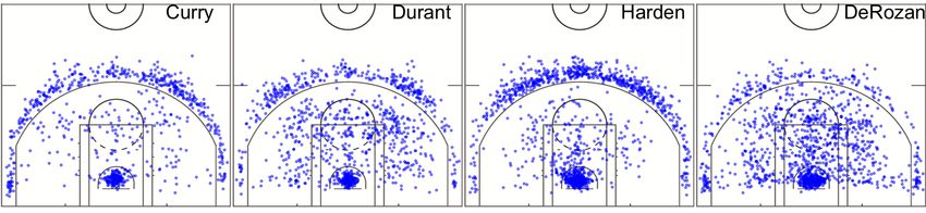
Figure 4: Shot data Display. On half court image, each point represents one shot. From left to right: Stephen Curry, Kevin
Durant, James Harden, DeMar DeRozan.
We visualize and summarize the shot data of four key players, Stephen Curry, James Harden, Kevin Durant and DeMar
DeRozan. Figure 4 shows their field goal attempts’ locations and Table 4 summarizes their other field goal attempts
information. As we can see from the plots, most of the shots are made either close to the rim or right outside the arc (i.e.,
3-point line). This is in line with the recent trend in the basketball development since it is more efficient for players to
pursue higher success rates near the rim or go after higher rewards by making 3-point shots.Bayesian Nonparametric Learning for Point Processes
Table 4: Shot data summary. Period is for the 1st, 2nd, 3rd, 4th quarter and the extra time. The 2PT shot percentage (%)
column gives the percentage of all shots that are 2 PT shots.
Player Shot Count 2PT shot percentage (%) Period percentage (%)
Stephen Curry 753 42.6 (35.0, 20.6, 34.3, 9.7, 0.4)
James Harden 1306 50.2 (28.7, 22.4, 27.9, 20.8, 0.3)
Kevin Durant 1040 66.5 (30.8, 23.8, 30.6, 14.6, 0.3)
DeMar DeRozan 1274 79.9 (29.1, 28.6, 33.3, 17.3, 1.6)
E. More real data results
F. Histograms of K
b in simulation study
F.1. Simulation study, grid size: 20 × 20
eta=0 BIC DIC LPML MFM-NHPP
75
Setting 1
50
25
0
75
Setting 2
count
50
25
0
75
Setting 3
50
25
0
0 25 50 75 100 0 25 50 75 100 0 25 50 75 100 0 25 50 75 100 0 25 50 75 100
^
K
method eta=0 BIC DIC LPML MFM-NHPP
b from the 100 replicates for each simulation setting (grid size: 20 × 20), under MFM-NHPP,
Figure 7: Histograms of K
and MRF-DPM-NHPP with η = 0, optimal η selected by BIC, DIC and LPML. The blue vertical line indicates the true
number of clusters (K).Bayesian Nonparametric Learning for Point Processes
Table 5: Basic information (name and the preferred position) of players and the number of clusters given by MRF-DPM-
NHPP with the smoothing parameter selected by BIC, and by MFM-NHPP. Player positions: point guard (PG), shooting
guard (SG), small forward (SF), power forward (PF), center (C).
MRF-DPM-NHPP MFM-NHPP
Player Position K
b BIC ηbBIC K
b
DeAndre Jordan C 7 2.5 5
Joel Embiid C 7 3.5 10
Karl-Anthony Towns C 12 3.0 12
Dwight Howard C 6 3.0 5
Giannis Antetokounmpo PF 8 3.0 16
Blake Griffin PF 6 3.0 4
LaMarcus Aldridge PF 7 4.0 11
Kristaps Porziņgis
‘
PF 6 3.0 11
Stephen Curry PG 6 3.0 9
Damian Lillard PG 8 3.0 9
Chris Paul PG 6 5.0 8
Kyrie Irving PG 8 3.0 9
Kevin Durant SF 9 3.5 10
LeBron James SF 8 3.0 14
Paul George SF 9 3.0 9
Jimmy Butler SF 8 3.5 12
James Harden SG 7 4.0 11
DeMar DeRozan SG 10 3.0 10
Russell Westbrook SG 7 3.0 13
Klay Thompson SG 6 3.0 14Bayesian Nonparametric Learning for Point Processes
C C C C
Embiid Howard Jordan Towns
PF PF PF PF
Aldridge Antetokounmpo Griffin Porzingis
PG PG PG PG
Curry Irving Lillard Paul
SF SF SF SF
Butler Durant George James
SG SG SG SG
DeRozan Harden Thompson Westbrook
log(intensity)
−6 −4 −2 0 2 4
Figure 5: Estimated shooting log-intensity surfaces of selected players based on MRF-DPM-NHPP.Bayesian Nonparametric Learning for Point Processes
C C C C
Embiid Howard Jordan Towns
PF PF PF PF
Aldridge Antetokounmpo Griffin Porzingis
PG PG PG PG
Curry Irving Lillard Paul
SF SF SF SF
Butler Durant George James
SG SG SG SG
DeRozan Harden Thompson Westbrook
log(intensity)
−8 −4 0 4
Figure 6: Estimated shooting log-intensity surfaces of selected players based on MFM-NHPP.Bayesian Nonparametric Learning for Point Processes
F.2. Simulation study, grid size: 50 × 35
eta=0 BIC DIC
30
20
10
0
count
0 100 200 300
LPML MFM−NHPP
30
20
10
0
0 100 200 300 0 100 200 300
^
K
method eta=0 BIC DIC LPML MFM−NHPP
b from the 100 replicates for simulation setting ((grid size: 50 × 35)), under MFM-NHPP, and
Figure 8: Histograms of K
MRF-DPM-NHPP with η = 0, optimal η selected by BIC, DIC and LPML. The blue vertical line indicates the true number
of clusters (K).Bayesian Nonparametric Learning for Point Processes G. Traceplots of RI between ground truth and each partition in simulation study G.1. Simulation study, grid size: 20 × 20 Figure 9: Overlaid trace plots of RI between the truth and the partition obtained at each iteration from 100 replicates for each simulated setting under grid size 20 × 20. The thick lines are the average traces over the 100 replicates.
Bayesian Nonparametric Learning for Point Processes

G.2. Simulation study, grid size: 50 × 35

Figure 10: Overlaid trace plots of RI between the truth and the partition obtained at each iteration from 100 replicates for
the simulation setting under grid size 50 × 35. The thick lines are the average traces over the 100 replicates.
Bayesian Nonparametric Learning for Point Processes

G.3. Traceplots of estimated intensity at pixel (25,6) in NBA data analysis - full data

Figure 11: Traceplots of estimated intensity at pixel (25,6) for NBA data analysis after burnin and thinning for two inde-
pendent chains.
Bayesian Nonparametric Learning for Point Processes

G.4. Traceplots of Adjusted RI between successive partitions in NBA data analysis - full data

Figure 12: Traceplots of adjusted RI between successive partitions for NBA data analysis after burnin and thinning for two
independent chains.
You can also read