Bayesian approach for predicting photogrammetric uncertainty in morphometric measurements derived from drones
←
→
Page content transcription
If your browser does not render page correctly, please read the page content below
Vol. 673: 193–210, 2021            MARINE ECOLOGY PROGRESS SERIES
                                                                                                  Published September 2
https://doi.org/10.3354/meps13814                 Mar Ecol Prog Ser

                                                                                                    OPEN
                                                                                                    ACCESS

Bayesian approach for predicting photogrammetric
   uncertainty in morphometric measurements
              derived from drones
             K. C. Bierlich1, 2,*, R. S. Schick1, J. Hewitt3, J. Dale1, J. A. Goldbogen4,
                                 A. S. Friedlaender5, D. W. Johnston1
 1
     Division of Marine Science and Conservation, Nicholas School of the Environment, Duke University Marine Laboratory,
                                                 Beaufort, North Carolina 28516, USA
              2
                Marine Mammal Institute, Department of Fisheries, Wildlife, & Conservation, Oregon State University,
                                  Hatfield Marine Science Center, Newport, Oregon 97365, USA
                     3
                       Department of Statistical Science, Duke University, Durham, North Carolina 27708, USA
            4
             Department of Biology, Hopkins Marine Station of Stanford University, Monterey, California 93950, USA
      5
       Institute of Marine Sciences, Department of Ecology and Evolutionary Biology, University of California Santa Cruz,
                                                  Santa Cruz, California 95604, USA

         ABSTRACT: Increasingly, drone-based photogrammetry has been used to measure size and body
         condition changes in marine megafauna. A broad range of platforms, sensors, and altimeters are
         being applied for these purposes, but there is no unified way to predict photogrammetric uncer-
         tainty across this methodological spectrum. As such, it is difficult to make robust comparisons
         across studies, disrupting collaborations amongst researchers using platforms with varying levels
         of measurement accuracy. Here we built off previous studies quantifying uncertainty and used an
         experimental approach to train a Bayesian statistical model using a known-sized object floating at
         the water’s surface to quantify how measurement error scales with altitude for several different
         drones equipped with different cameras, focal length lenses, and altimeters. We then applied the
         fitted model to predict the length distributions and estimate age classes of unknown-sized hump-
         back whales Megaptera novaeangliae, as well as to predict the population-level morphological
         relationship between rostrum to blowhole distance and total body length of Antarctic minke
         whales Balaenoptera bonaerensis. This statistical framework jointly estimates errors from altitude
         and length measurements from multiple observations and accounts for altitudes measured with
         both barometers and laser altimeters while incorporating errors specific to each. This Bayesian
         model outputs a posterior predictive distribution of measurement uncertainty around length
         measurements and allows for the construction of highest posterior density intervals to define
         measurement uncertainty, which allows one to make probabilistic statements and stronger infer-
         ences pertaining to morphometric features critical for understanding life history patterns and
         potential impacts from anthropogenically altered habitats.

         KEY WORDS: Bayesian modeling · Photogrammetry · Uncertainty analysis · Drones · Unoccupied
         aircraft system · UAS · Morphometrics · Marine mammals · Cetaceans

                   1. INTRODUCTION                               health, likelihood of survival, and potential reproduc-
                                                                 tive success of an individual (Arnold 1983, Irschick
  The morphology of an animal is one of the most                 2003). Collecting accurate morphological measure-
fundamental factors affecting its habitat use and forag-         ments of individuals is often essential for monitoring
ing performance, and can reflect details of the current          populations, and recent studies have demonstrated
                                                                 © The authors 2021. Open Access under Creative Commons by
                                                                 Attribution Licence. Use, distribution and reproduction are un-
*Corresponding author: kevin.bierlich@oregonstate.edu
                                                                 restricted. Authors and original publication must be credited.
                                                                 Publisher: Inter-Research · www.int-res.com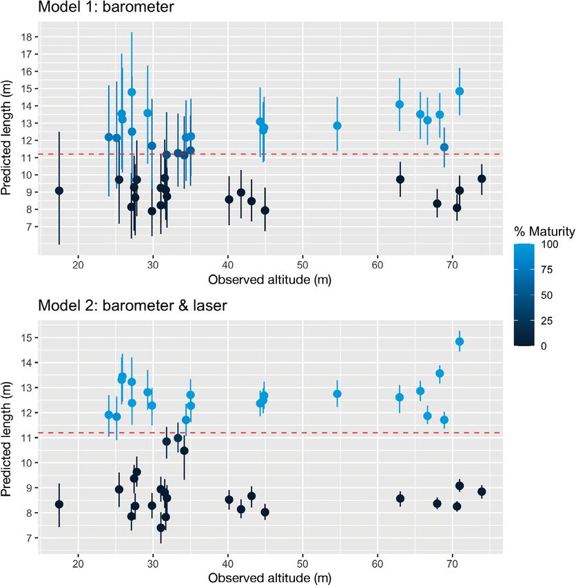
194                                      Mar Ecol Prog Ser 673: 193–210, 2021

how animal morphology has profound implications              living cetaceans by Whitehead & Payne (1981). Pho-
for conservation and management decisions, espe-             tographs of southern right whales next to a boat with
cially for populations inhabiting anthropogenically          a known-sized disc were collected to set the scale of
altered environments (De Meyer et al. 2020, Miles            the photograph (Whitehead & Payne 1981). This
2020). However, obtaining accurate morphometric              method was later enhanced by using altimeters to
measurements of marine megafauna is challenging,             record the altitude and set the scale of the photo-
particularly for cetaceans, as they are often found in       graph by calculating the ground sampling distance
remote locations, spend little time at the surface of        (GSD), the distance on the ground that each pixel
the water, and their large size can preclude safe cap-       represents (Cubbage & Calambokidis 1987, Best &
ture and live handling (Johnston 2019).                      Rüther 1992). These methods have been commonly
   Recently, unoccupied aircraft systems (UAS), or           used to obtain length measurements of odontocetes
drones, have proven to be a valuable, non-invasive           and mysticetes (Perryman & Lynn 1993, Ratnaswamy
tool for collecting high-resolution photogrammetric          & Winn 1993, Perryman & Westlake 1998, Fearnbach
data on cetaceans across a variety of ecosystems.            et al. 2011, 2018), as well as width measurements to
Durban et al. (2015) first demonstrated the utility of       assess nutritive condition related to reproduction in
using UAS for acquiring morphometric measure-                gray whales (Perryman & Lynn 2002) and southern
ments of killer whales Orcinus orca in a remote loca-        and North Atlantic right whales (Miller et al. 2012).
tion with limited occupied aircraft support. Since then,        Compared to occupied aircraft, UAS have greatly
UAS have been used from tropical to polar environ-           enhanced opportunities to more efficiently collect
ments and applied to several cetacean species of vastly      high-resolution aerial photogrammetric data on ceta-
different sizes and body shapes, including blue whales       ceans, as they offer a more affordable (Arona et al.
Balaenoptera musculus, humpback whales Mega-                 2018) and immediate option that is less limited by
ptera novaeangliae, southern right whales Eubalaena          weather and infrastructure (e.g. Cosens & Blouw 2003,
australis, North Atlantic right whales E. glacialis, gray    Fearnbach et al. 2011), and, importantly, presents
whales Eschrichtius robustus, fin whales B. physalus,        less risk to wildlife biologists (Sasse 2003). However,
Antarctic minke whales B. bonaerensis, and Bryde’s           many studies use different UAS platforms equipped
whales B. brydei (Christiansen et al. 2016, 2018,            with various cameras and focal length lenses, which
2020a,b, Durban et al. 2016, Gough et al. 2019, Lemos        have inherent differences in lens distortion (i.e. Bur-
et al. 2020). However, a broad range of UAS plat-            nett et al. 2019) and GSD (see Fig. 1). These different
forms, sensors, and altimeters were applied in these         platforms and sensors vary in performance, quality,
studies, and there is no unified way to predict pho-         and photogrammetric accuracy; to date, a rigorous
togrammetric uncertainty across this methodological          analysis of the impact of these factors has not been
spectrum. As such, it is difficult to make robust com-       undertaken.
parisons among studies, disrupting collaborations               In the USA, the National Institute of Standards and
amongst researchers using platforms with varying             Technology (NIST) provides guidelines put forth by
levels of measurement accuracy. As the capacity to           the International Committee for Weights and Meas-
collect morphometric data on various species via UAS         ures (CIPM) for how to report measurements and
continues to grow, there is a need for standardization       uncertainty, as a measurement result is complete
of measurements across studies and minimization              only when accompanied by a quantitative statement
and quantification of errors (Castrillon & Bengtson          of its uncertainty (Taylor & Kuyatt 1994). In the con-
Nash 2020). This will ultimately build a greater capac-      text of collecting aerial imagery of cetaceans for mor-
ity to better monitor populations exposed to a variety       phometric analysis, measurement errors can be intro-
of environmental and anthropogenic stressors.                duced by environmental conditions (e.g. glare, wave
   Traditional methods for acquiring morphometric            refraction, water clarity) and animal behavior (e.g.
measurements of cetaceans have previously been               curved vs. straight body at depth/at surface). These
limited to carcasses collected from scientific whaling       errors are largely uncontrollable, but they can be
operations (Ichii & Kato 1991) or opportunistically from     mitigated, such as by avoiding flying during times
commercial whaling (Lockyer 1981, Christiansen et            with high glare and filtering for high-quality images
al. 2013), subsistence hunting (Lambertsen et al. 2005),     where the animal is straight at the surface with min-
stranding events (Palacios et al. 2004), and bycatch         imal refraction from waves (Christiansen et al. 2018,
(Read 1990, Koopman et al. 2002). Aerial photogram-          Burnett et al. 2019, Raoult et al. 2020). It then becomes
metry from occupied aircraft was adopted as a non-           important to understand components in the UAS
invasive technique for estimating the length of free-        photogrammetric workflow that can be controlled to
Bierlich et al.: Predicting photogrammetric uncertainty                             195

minimize systematic errors associated with the UAS               Here, we built off the studies of Burnett et al. (2019)
platform and analysis.                                        and Christiansen et al. (2018) and developed a
   In general, assessment of measurement error has            Bayesian statistical model that propagates the com-
focused on measuring the length of a known-sized              bined impact of measurement errors to UAS pho-
object either on land (Best & Rüther 1992, Perryman           togrammetric measurements and derived quantities,
& Lynn 1993, Christiansen et al. 2018), floating at the       such as length-based age classifications (e.g. juve-
surface (Perryman & Lynn 2002, Burnett et al. 2019,           nile/adult). Similar to Racine-Poon (1988), we used a
Gough et al. 2019, Kahane-Rapport et al. 2020), or on         designed experiment to generate training data for
a research vessel (Durban et al. 2015, 2016) to quan-         the Bayesian statistical model. The experiment used
tify errors associated with altimeters and analyst            a known-sized object floating at the surface to study
measurements. These different forms of data collec-           how measurement error scales with altitude for sev-
tion can lead to significant biases in reported meas-         eral different UAS platforms equipped with different
urement errors associated with altimeters on UAS,             cameras, focal length lenses, and altimeters. We then
which can have different accuracies depending on              applied the fitted model to 2 ecological scenarios in
altitude and ground elevation, and whether the UAS            which we (1) predicted the length and measurement
are flown over land or sea (Dawson et al. 2017).              uncertainty around unknown-sized humpback whales
Many studies have accounted for altimeter error by            to assign maturity classification, and (2) predicted the
using correction coefficients from a linear equation          population-level morphological relationship between
(Best & Rüther 1992, Perryman & Lynn 1993) or by              rostrum to blowhole distance and total length of
applying a percent error to all measurements (Rat-            Antarctic minke whales. The Bayesian model offers
naswamy & Winn 1993), e.g. error value of < 5% for            several components that improve uncertainty predi-
all measurements. Since the true length of the whale          cations. First, the model provides a framework that
is unknown, the coefficient of variation (CV) is often        jointly estimates errors from altitude and length
used to determine the within-frame and between-               measurements. Second, the model combines altitude
frame measurement precision. Within-frame preci-              measured with a barometer and laser altimeter while
sion compares measurements of the same whale in a             incorporating the different errors specific to each.
single image multiple times, often by multiple ana-           Third, rather than a single point-estimate, the model
lysts, while between-frame precision compares meas-           outputs a posterior predictive distribution of meas-
urements of the same whale between different images           urements around an object of unknown length (e.g. a
(Cosens & Blouw 2003).                                        whale). Fourth, this approach allows for the construc-
   Recently, Christiansen et al. (2018) used a frequen-       tion of highest posterior density (HPD) interval to
tist statistical approach to first measure a known-           define measurement uncertainty, which allows one
sized object at altitudes between 5 and 120 m and             to make probabilistic statements and reach stronger
then used resampling methods to build an error dis-           conclusions, e.g. classification of the maturity of an
tribution around measurements of southern right               animal based on its estimated length. Finally, we pro-
whales described by laser altimeter error, image              vide a framework that can easily incorporate addi-
quality, and the CV of within- and between-image              tional modeling layers. For example, at the data col-
measurements. Similarly, Burnett et al. (2019) used           lection level, the effect of additional covariates on
known-sized objects to first independently estimate           measurement error can be studied; or, at the scien-
the variance around altitude recorded from barome-            tific level, morphological relationships can be jointly
ters on small low-cost UAS and measured length,               estimated alongside measurement error.
and then estimated total measurement error via vari-
ance propagation. While these methods greatly im-
prove error estimation, both assume that errors are                     2. MATERIALS AND METHODS
independent and adequately described by their stan-
dard deviations and CVs (Christiansen et al. 2018,                2.1. Calculating Ground Sampling Distance
Burnett et al. 2019). The apparent length of an object
is dependent on altitude, and errors may have more              The GSD sets the scale of the photo in order to con-
complicated features (e.g. skew, and heavy tails or           vert measurements made in pixels into standard
outliers). Methods that account for these issues may          units (i.e. meters) by using the following equations
further improve estimates of measurement error                (see Torres & Bierlich 2020 for review):
across UAS platforms, and facilitate error propaga-                                      a S
                                                                                  GSD = × w                       (1)
tion to additional, derived quantities.                                                  fc I w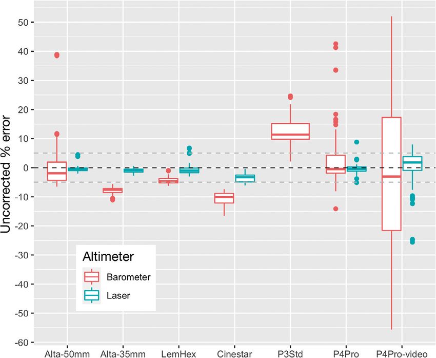
196 Mar Ecol Prog Ser 673: 193–210, 2021
Length = GSD × Lp (2) eral studies have improved the accuracy of the alti-
where a is altitude, which is the distance (m) from the tude recorded by using a laser altimeter, e.g. Light-
camera to the object of interest (i.e. the whale is as- Ware SF11/C LIDAR (Dawson et al. 2017), or by
sumed to be flat at the surface of the water), fc is the measuring a known-sized object during each flight to
focal length of the camera (mm), Sw is the sensor correct for barometric altitude inaccuracies using lin-
width of the camera (mm), Iw is the image width (pix- ear equations (Burnett et al. 2019, Lemos et al. 2020).
els, px), and Lp is the length (px) of the object of inter-
est. As altitude increases, GSD also increases, ulti-
mately decreasing the resolution of the image, which 2.1.1. Training and calibration data (x)
can influence Lp measurement accuracy as specific
features and edges of the whale become more diffi- Seven UAS flights were conducted on 26 June
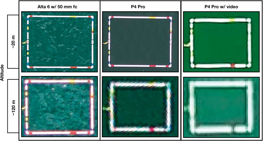
cult to identify (see Figs. 1 & 2). Furthermore, differ- 2019 at the Duke University Marine Lab in Beaufort,
ent methods of data collection (i.e. collecting still NC, USA (34° 43’ 0.156’’ N, 76° 40’ 24.42’’ W) and are
images vs. video) will also change the GSD for the detailed in Table 1. Each aircraft was launched from
same camera, as video uses fewer pixels in the image a dock ~100 m from a known-sized floating calibra-
width (Iw) compared to still images, ultimately de- tion object made of PVC pipe (1.48 m × 1.15 m). The
creasing resolution and increasing the GSD (Eq. 1, calibration frame was foam-filled to maintain flota-
Fig. 1). tion at the surface of the water and anchored via rope
In Eq. (1), the camera parameters (Sw, Iw, fc) are with a buoy to prevent drifting. The site was chosen
fixed and can be accounted for. The other parameter, because it is sheltered from ocean swell and thus
altitude (a), has the greatest influence on determin- ensured the calibration frame remained relatively
ing GSD. This is potentially a major source of meas- flat at the surface during data collection. Prior to
urement error due to discrepancies in the correct takeoff, the launch height was measured from the
scaling of the pixels in the image caused by altimeter water surface to the camera lens and then later
errors (Burnett et al. 2019). All UAS are equipped added to the recorded barometer altitude to account
with a barometer, which is a pressure sensor for re- for the bias introduced from the barometer zeroed at
cording altitude, but each will have some level of launch height (see Durban et al. 2015) and the local
inaccuracy when measuring and recording true alti- rising tide. Each aircraft collected imagery of the cal-
tude. Recording the offset from launch height to the ibration frame at altitudes between 10 and 120 m in
water is critical, as the barometer sets the zero pres- 10 m increments, similar to Christiansen et al. (2018).
sure at the takeoff point. Flying from land also adds For the P4Pro flight with video, a still frame was cap-
complications with allowance for altitude offsets due tured using the snapshot function in VLC Media
to tidal fluctuations. Generally speaking, lower accu- Player Software (Version 3.08, VideoLAN), as in
racy usually arises from the use of low-cost sensors Lemos et al. (2020). To test for possible effects of lens
commonly found on small UAS (Wei et al. 2016). Sev- distortion at various altitudes, the calibration frame
Fig. 1. Ground sampling distance
(GSD) for unoccupied aircraft sys-
tem (UAS) platforms commonly
used for cetacean photogramme-
try. The GSD displayed is exact,
meaning it does not account for
distortion or altitude errors. GSD
increases with increasing alti-
tude, lowering image resolution.
See Table 1 for list of UAS plat-
forms used in this current study;
px: pixel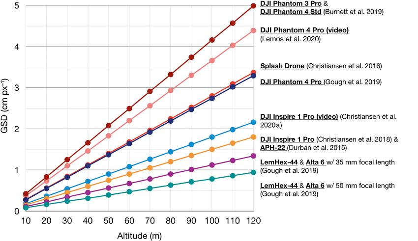
Bierlich et al.: Predicting photogrammetric uncertainty 197
was positioned in the center of the image during the
Table 1. Camera specifications for each flight and aircraft. All aircraft contained a barometer and laser altimeter, except for Phantom 3 Std. The Olympus EPM2 camera
f/2.8−f/11
f/2.8−f/11
f-number
ascent and in the corner during the descent. We also
f/2.8
f1.8
f1.8
f1.8
f1.8
tested the distortion of each camera using the Math-
Works Single Camera Calibrator App in MATLAB,
following the provided tutorial (MathWorks 2017)
0.00392 × 0.00390
0.00392 × 0.00390
0.00392 × 0.00390
0.00375 × 0.00376
0.00241 × 0.00286
0.00322 × 0.00407
0.00154 × 0.00154
Pixel dimensions and Burnett et al. (2019).
(mm px−1)
In addition to an onboard barometer, each aircraft
except for the P3Std was equipped with a LightWare
SF11/C laser altimeter that simultaneously recorded
altitude along with the barometer (Table 1). A cus-
tom designed housing was created to support and
power the laser altimeter on the P4Pro (installation
has also been used on other UAS platforms, e.g. APH-22 (Durban et al. 2015, 2016). px: pixel
Image dimensions
instructions at https://github.com/marrs-lab/DJI_PH4_
6000 × 4000
6000 × 4000
6000 × 4000
4608 × 3456
5472 × 3078
4096 × 2160
4000 × 3000
LaserAltimeter). The LightWare SF11/C laser altime-
ter is rated for altitude measurements up to 120 m
(px)
above land and 40 m above moving water with ±0.1 m
of error (LightWare Optoelectronics 2018). Each plat-
form contained the laser altimeter and camera co-
located on a 2-axis gimbal with pitch angle con-
sensor (mm)
13.20 × 8.80
13.20 × 8.80
trolled via remote control to ensure image collection
23.5 × 15.6
23.5 × 15.6
23.5 × 15.6
6.16 × 4.62
17.3 × 13
Camera
at nadir, except for P4Pro, which had the laser fixed
on the aircraft frame, and we accounted for the pitch
and roll to calculate the vertical altitude during
image collection (Dawson et al. 2017). Timestamp
Focal length
drift can lead to improper scaling of images due to
(mm)
incorrect altitudes used in calculating GSD (Voges et
3.61
8.8
8.8
50
35
35
25
al. 2018, Raoult et al. 2020). To correct for this, we
took images of an iPad screen connected to a Bad Elf
GPS unit displaying the current GPS time prior to
Olympus EPM2
Phantom 4 Pro
Phantom 4 Pro
Phantom 3 Std
take off. This ensures we can accurately link the
Sony a5100
Sony a5100
Sony a5100
Camera
timestamp of an image to the altitude recorded by
the barometer and laser altimeter.
2.1.2. Photogrammetry
Barometer & Laser
Barometer & Laser
Barometer & Laser
Barometer & Laser
Barometer & Laser
Barometer & Laser
Barometer
Altimeter
The length of the calibration frame was measured
in pixels (Lp’) using the straight-line tool in ImageJ
1.5i (Schneider et al. 2012) by 3 separate analysts (2
considered ‘expert’, one considered ‘novice’). To as-
sess measurement bias between analysts, the coeffi-
cient of variation (CV%) was calculated between the
collected
Images
Images
Images
Images
Images
Images
Video
3 Lp’ measurements for each image, following the
Data
approach of Christiansen et al. (2016).
To compare the measurement error amongst differ-
ent UAS platforms, i.e. to derive the uncorrected
Phantom 4 Pro
Phantom 4 Pro
Phantom 3 Std
Lemhex-44
measurement error, we used Eqs. (1) and (2) to con-
CineStar
Aircraft
Alta 6
Alta 6
vert each Lp’ measurement into 2 length measure-
ments (m), one using the altitude recorded from the
barometer and one from the laser altimeter. The
uncorrected percent error was then calculated as:
Flight
(Lp,ijk ’ − Lco )
uncorrected % error = × 100
1
2
3
4
5
6
7
(3)
Lco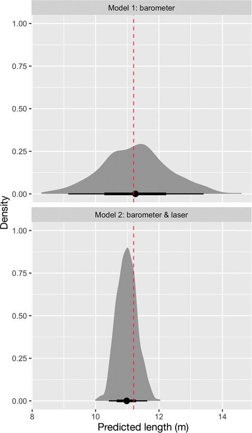
198                                             Mar Ecol Prog Ser 673: 193–210, 2021

where Lco is the true length of the calibration object              experimental study of measurement errors for a
(1.48 m) and Lp,ijk’ is the length (px) of the calibration          given UAS platform.
object in each image i, measured by analyst j, using
altimeter k (barometer or laser) (Christiansen et al.
2018, Burnett et al. 2019).                                                            2.2.2. Error estimation

                                                                       We used Eqs. (1) and (2) to design the likelihood
               2.2. Model development                               function. We assumed that L, a, and Lp represent the
                                                                    length of a target object, the exact altitude at which
       2.2.1. Overview of Bayesian approach                         an image is taken, and the length of the object in the
                                                                    image, in pixels, respectively. The data x = (aL’, aB’,
  Unlike frequentist statistical theory, the Bayesian               Lp’) are the altitude as measured by a laser altimeter
approach views both data and the underlying para-                   (aL’) and barometer (aB’), and the measured length of
meters (i.e. variances) that generated the data as ran-             the object in the image, in pixels (Lp’), all of which
dom (see Austin et al. 2002 and Ellison 2004 for re-                represent noisy versions of the exact values a and Lp,
views). Using Bayes’ theorem, a model of the observed               respectively. We assigned a uniform prior distribu-
data, called the likelihood function, is combined with              tion to a (min = 5 m and max = 130 m), which restricts
prior knowledge pertaining to the underlying para-                  the model to the altitude range of UAS image collec-
meters, called the prior probability distribution, to               tion but is otherwise uninformative. We expect most
form the posterior probability distribution. The poste-             altimeter measurement errors are smaller than a few
rior probability distribution serves as updated knowl-              meters at worst, and that the errors are normally dis-
edge about the underlying parameter and can be                      tributed around the true altitude a such that:
used as prior information for subsequent studies.                                           aL’ ~ N(a,σL2 )                 (6)
  Following this framework, we first estimated the
posterior probability distribution for a vector of pho-                                     aB’ ~   N(a,σB2 )               (7)
togrammetric error parameters (θ) from different                       The altimeters have separate variance parameters
UAS platforms using calibration data (x) of a known                 σL2 and σB2, to each of which we assign an inverse
sized object via:                                                   gamma prior distribution (shape = 2, rate = 1). Meas-
                                 ƒ(x | θ)ƒ(θ)                       urement error is assumed to have constant variance
                   ƒ(θ | x ) =                              (4)     over unknown altitudes, which simplifies modeling
                                    ƒ(x )
                                                                    and estimation. Impacts of the constant variance as-
where ƒ(x|θ) is the likelihood function, ƒ(θ) is the prior          sumption are evaluated in model validation (Section
probability distribution that defines the potential                 2.3.1).
range for θ, ƒ(x) is the marginal distribution of the                  We also assumed the measured length of the object,
measurement data, and ƒ(θ|x) is the posterior distri-               in pixels, Lp’ is normally distributed around the exact
bution that defines the likely range of θ given data x.             value Lp by specifying the prior distribution:
We designed the likelihood function to account for                                                     2
                                                                                           Lp’ ~ N(Lp,σLp )                 (8)
sources of UAS measurement error (see Section 2.2.2).
Taking a similar approach as Racine-Poon (1988), we                 to which we assigned an inverse gamma prior distri-
then used the posterior probability distributions for θ,            bution (shape = 5, rate = 4) for the variance parame-
specific to UAS platform, as prior information to form              ter σLp
                                                                          2
                                                                            . Eqs. (1) and (2) imply that the exact length of
posterior predictive distributions for measurements                 the object in pixels, Lp, depends on the length L of
of an unknown-sized object (L new) from observations                the target object and the altitude at which the image
(xnew) collected in the field (e.g. of whales) using that           is taken (a) via:
UAS platform via:
                                                                                                  L × fc × I w
                                                                                           Lp =                             (9)
       ƒ(L new|x,xnew) = ∫ ƒ(L new|θ,xnew) ƒ(θ|x)dθ         (5)                                     a × Sw
where ƒ(L new|θ,xnew) is a conditional likelihood, and                The length L of the target object is known in the
ƒ(θ|x) is the posterior probability distribution from               calibration experiment, yielding the likelihood:
Eq. (4), which effectively serves as an updated prior
                                                                         ƒ(θ|x) = ∫ ƒ(a) ƒ(aL’|a,θ) ƒ(aB’|a,θ) ƒ(Lp’|a,θ)da (10)
probability distribution. The posterior predictive dis-
tribution ƒ(L new|x,xnew) quantifies uncertainty in meas-           in which ƒ(a) is the uniform prior density for the true
urements of an unknown-sized object based on the                    altitude, ƒ(aL’|a,θ) and ƒ(aB’|a,θ) are the densities for
Bierlich et al.: Predicting photogrammetric uncertainty 199
the altimeter measurement errors (Eqs. 6 and 7), scenario, we randomly split the LemHex-44 and Alta
ƒ(Lp’|a,θ) is the measurement error distribution of the 6 data (collected in Section 2.1.1) into equal-sized
pixel length (Eq. 8), the parameter vector is θ = (σL2, training and testing subsets. In the second scenario,
σB2, σLp
2
), and the calibration object length L co is sub- we ensured the training and testing subsets were
stituted for L in Eq. (9). We then can use measure- also balanced with respect to images taken at low,
ments of L co as training data to estimate error para- medium, and high altitudes (respectively 0−30, 31−
meters θ specific to UAS platforms. 60, and 61−120 m). To be precise, the LemHex-44
and Alta 6 data included 42 images nominally taken
at altitudes between 0 and 30 m; the second scenario
2.2.3. Measurement predictions ensured that the training and testing subsets each
had 21 of these images, while the first scenario did
After estimating θ, we can use the posterior predic- not. The first scenario is more general, while the sec-
tive distribution (Eq. 5) to make inferences about the ond scenario allows out-of-sample prediction error to
size of an unknown object (L new), e.g. length of a whale, be studied with respect to altitude.
which is conditional on a new set of measurements In both scenarios, we used the training subset to
xnew = (aL,new’, aB,new’, Lp,new’) and our error parameter estimate the error parameters 3 separate times: when
estimates from the UAS platforms used in data col- altitude information is taken from (1) both the barom-
lection. The conditional likelihood ƒ(L new |θ,xnew) in eter and laser altimeters, (2) only the barometer, and
Eq. (5) is formed from Bayes’ rule. The rule implies (3) only the laser. We used each set of parameter esti-
the known-length likelihood (Eq. 10) is weighted by mates to predict the length measurements of the test-
the prior distribution for the unknown object length ing subset. Next, we compared the predicted lengths
ƒ(L new), and is proportional to: to the known length of the calibration object (L co),
using root mean square error (RMSE) and mean
ƒ(L new|θ,x new) ∝ ƒ(xnew|θ,Lnew) ƒ(L new) (11)
absolute error (MAE) to summarize the prediction
in which ƒ(xnew|θ,L new) is the likelihood Eq. (10), but errors. Comparing the 3 sets of predictions lets us test
for which the unknown object length L new is substi- how altimeter choice influences uncertainty.
tuted for L in Eq. (9). We assigned a uniform prior dis-
tribution (min = 0 m, max = 30 m) to the unknown
lengths of humpback whales, which restricts the 2.3.2. Ecological scenarios
model to reasonable size ranges but is otherwise
uninformative. We discuss an alternate choice for We then tested the model in 2 ecological scenarios
ƒ(L new) in Section 2.3 that allows for estimation of to (1) predict total body length measurements of
morphological relationships between multiple length humpback whales (n = 48) in order to assign maturity
measurements. class, and (2) estimate the morphological relationship
Model development and analyses were conducted between total length and rostrum to blowhole dis-
in R (version 4.0.2, R Core Team 2020). Estimation tance of Antarctic minke whales (n = 27). Both sce-
and prediction were performed using Markov chain narios used images collected with the LemHex-44
Monte Carlo sampling in NIMBLE (de Valpine et al. (35 mm fc) (referred to as ‘LemHex’) and Alta 6 (re-
2017) with 1000 burn-in followed by 1 000 000 itera- ferred to as ‘Alta’) with either a 35 or 50 mm fc. Both
tions. Three independent chains were run to confirm scenarios compare predicted lengths under 2 models:
consistency between runs and inspected visually for Model 1 assumes that each platform contains only a
convergence. Model code is freely available at the barometer to record altitude for length measure-
Duke University Research Data Repository (https:// ments, whereas Model 2 assumes that each platform
doi.org/10.7924/r4sj1jj6s). has both a barometer and a laser altimeter. Images
were selected for each individual and ranked for
quality in measurability following Christiansen et al.
2.3. Testing data (L new) (2018), where a score of 1 (good quality), 2 (medium
quality), or 3 (poor quality) was applied to 7 attrib-
2.3.1. Model validation utes: camera focus, straightness of body, body roll,
body arch, body pitch, total length measurability,
We validated the ability of the model to estimate and body width measurability. Images with a score of
unknown lengths by studying the out-of-sample pre- 3 in any attribute were removed from analysis, as
diction error of the model in 2 scenarios. In the first well as any images that received a score of 2 in both200 Mar Ecol Prog Ser 673: 193–210, 2021
roll and arch, roll and pitch, or arch and pitch (Chris- photogrammetric data. The prior distribution is set to
tiansen et al. 2018). Data were collected along the restrict the support of measurements and parame-
Western Antarctic Peninsula between 2017 and 2019 ters, but is also large enough to be practically unin-
as part of long-term ecological research projects formative. We assumed RB measurements are linearly
focused on understanding population dynamics and related to TL measurements. The ith RB measure-
the impacts of interannual environmental variability ment, RBi , is modeled as a truncated normal random
on whale body condition. We used MorphoMetriX variable (min = 0 m, max = 30 m) with location
open-source photogrammetry software (Torres & parameter μi and scale parameter σRB2
via:
Bierlich 2020) to measure (in pixels) (1) the total 2
RBi |μi,σRB 2
~ trunc – N(μi,σRB ; 0, 30) (12)
length (TL), as tip of rostrum to fluke notch, of hump-
back and Antarctic minke whales, as well as (2) ros- μi = β1 + β2TLi (13)
trum to blowhole distance (RB) of Antarctic minke The location μi models the morphological relation-
whales. Both scenarios used the error parameters for ship between RBi and TLi, and the scale σRB 2
quanti-
the LemHex and Alta to generate posterior predic- fies the amount of population-level variability around
tive distributions for each measurement. Measure- the morphological relationship. The truncated range
ment uncertainty was defined by constructing 95% for RBi is the same as the original prior distribution
HPD intervals, which is an interval that represents ƒ(L new).
the region with a 95% probability of encompassing The prior distribution for the morphological rela-
the parameter. tionship is designed to be largely uninformative via:
2.3.2.1. Scenario 1: Predicting length-based matu- β1 ~ U(–3, 30) (14)
rity class. A single image was used for each individ-
β2 ~ Beta(1,1) (15)
ual to obtain length measurements. Length is often
used to classify individuals as mature or immature σRB
2
~ Inv-Gamma(0.01,100) (16)
(e.g. Christiansen et al. 2016, 2020a, Lemos et al. 2020). The prior distribution for the intercept β1 is mostly
Individuals were assigned as ‘mature’ if >50% of their non-negative, which strongly assumes that the inter-
predicted TL posterior distribution was greater than cept can be interpreted as a baseline size parameter.
the average length at maturity of 11.2 m, as used in The slope β2 quantifies the population-level ratio be-
previous studies (Christiansen et al. 2016, 2020a) that tween RB and TL, which is a priori known to beBierlich et al.: Predicting photogrammetric uncertainty 201
in which x and θ represent the collection of training There were clear resolution differences amongst
data and measurement error parameters as before, platforms due to GSD, especially with the DJI P4Pro
respectively; xRB,i and xTL,i represent the altitude and with video (Fig. 2). Differences in L p’ measurements
pixel-length measurements for RB and TL measure- of the same image amongst the 3 analysts were low,
ments, respectively; RBi and TLi represent the un- with CV < 5% for all measurements (min = 0.01%,
known RB and TL measurements, respectively, tak- max = 4.02%, mean = 0.87%, SD = 0.83%). Thus, the
ing the place of the generic object length L in previous analyst variable (within-frame precision) was ex-
equations; and the distributions comprise the likeli- cluded from the model.
hood and prior for a Bayesian analysis. We then com- Overall, each aircraft had greater uncorrected
pared the estimated morphological relationship and measurement error (before uncertainty model applied)
associated measurement uncertainty between Model when using the barometer for altitude compared to
1 (barometer only) and Model 2 (barometer and laser using the laser altimeter (Fig. 3; Table S2). The Alta
altimeter). with 50 mm fc had the lowest average uncorrected %
error compared to other platforms with the barometer,
but also had the third highest SD (Fig. 3; Table S2),
3. RESULTS likely due to an outlier at a low altitude (Fig. 3). The
mean uncorrected % error was reduced to202 Mar Ecol Prog Ser 673: 193–210, 2021
Fig. 3. Uncorrected % error for measurements from each unoccupied aircraft system (UAS) platform. Black dashed line repre-
sents 0% uncorrected error (true length = 1.48 m). The gray dashed lines represent the under- and over-estimation of the true
length by 5% (1.41 and 1.55 m, respectively). The middle line in each box represents the median (50th percentile), the lower
and upper hinges of the box represent the first and third quartiles (25th and 75th percentiles), respectively, and the lower and
upper whiskers represent the smallest and largest values that extend at most 1.5× the interquartile range. Any data beyond
these whiskers are considered outlying points and are plotted individually. Three analysts measured n images for each aircraft
using a barometer and laser: Alta 6 with 50 mm focal length lens (‘Alta-50mm’, nbarometer = 25, nlaser = 16), Alta 6 with 35 mm fo-
cal length lens (‘Alta-35mm’, nbarometer = 24, nlaser = 9), LemHex-44 (‘LemHex’, nbarometer = 25, nlaser = 23), Cinestar (nbarometer = 23,
nlaser = 20), P3Std (nbarometer = 24, nlaser = 0), P4Pro (nbarometer = 21, nlaser = 11), P4Pro w/ video (‘P4Pro-video’, nbarometer = 36, nlaser = 36)
object positioning (see Fig. S1). For this reason, object prediction error with respect to changing altitude, in-
positioning was removed from the model. Each cam- dicate that errors tend to decrease with altitude, but
era displayed low distortion (mean error ≤ 1.03 pixels) that the differences are scientifically negligible for
and was thus assumed negligible for incorporating in large animals (Table S3). In both scenarios, errors
the model. were nearly identical when using only a laser altime-
ter and using both a barometer and laser altimeter, in-
dicating that the laser altimeter results in lower meas-
3.2. Measurement predictions urement uncertainty (Table 2; Table S3).
3.2.1. Model validation Table 2. Results from validation test comparing how altime-
ter choice influences uncertainty predictions by comparing
the root mean square error (RMSE) and mean absolute error
The model validation study compared the model
(MAE) of the predicted measurements using altitude from
when altitude is collected using different altimeters only the barometer, only the laser altimeter, and both the
(barometer only, laser only, and both barometer and barometer and laser altimeter
laser) under 2 scenarios. Results from the first scenario,
which looks at overall prediction error, shows that er- RMSE (m) MAE (m)
rors are typically small across altimeters, with RMSE
and MAE < 0.08 m, although using only the barometer Barometer only 0.072 0.062
Laser altimeter only 0.021 0.014
had larger RMSE and MAE values (Table 2). Results
Barometer and laser altimeter 0.021 0.016
from the second scenario, which allows us to studyBierlich et al.: Predicting photogrammetric uncertainty 203
3.2.2. Ecological Scenario 1 of altimeter choice and incorporating uncertainty
into maturity classification. Overall, Model 1 (barom-
We predicted length distributions of humpback eter only) predicted longer measurements with much
whales (n = 48) using altitude from only a barometer greater uncertainty compared to Model 2 (barometer
(Model 1) and from both a barometer and laser alti- and laser altimeter), across all individuals (Fig. 5).
meter (Model 2) to assign sexual maturity. An exam- Each 95% HPD interval quantifies the most likely
ple of an individual’s posterior predictive length dis- range in which an exact measurement lies. As such,
tribution and 95% HPD intervals from Models 1 and we can represent the total uncertainty in each meas-
2 is shown in Fig. 4. This individual would be classi- urement using the width of the estimated 95% HPD
fied as ‘mature’ if using Model 1, but as ‘immature’ if interval. Model 1 predicted wider 95% HPD inter-
using Model 2. This result highlights the importance vals (mean ± SD = 3.81 ± 1.47 m, min = 1.52 m, max =
6.84 m) compared to Model 2 (1.10 ± 0.42, min =
0.42 m, max = 2.00 m) (Figs. 5 & 6). These wider pre-
dictive distributions from Model 1 resulted with more
overlap across the 11.2 m maturity cutoff length, with
several points in particular that would be considered
‘mature’ if using Model 1, but ‘immature’ if using
Model 2 (Fig. 5). These results suggest that when
measurements are made solely with the barometer,
extra caution needs to be taken to classify measured
individuals into different life-history classes. The
widths of the 95% HPD intervals decreased as alti-
tude increased for both models (Figs 5 & 6). All un-
corrected total length measurements (before applying
the uncertainty model) fit within the respective 95%
HPD interval of each individual (Fig. S2).
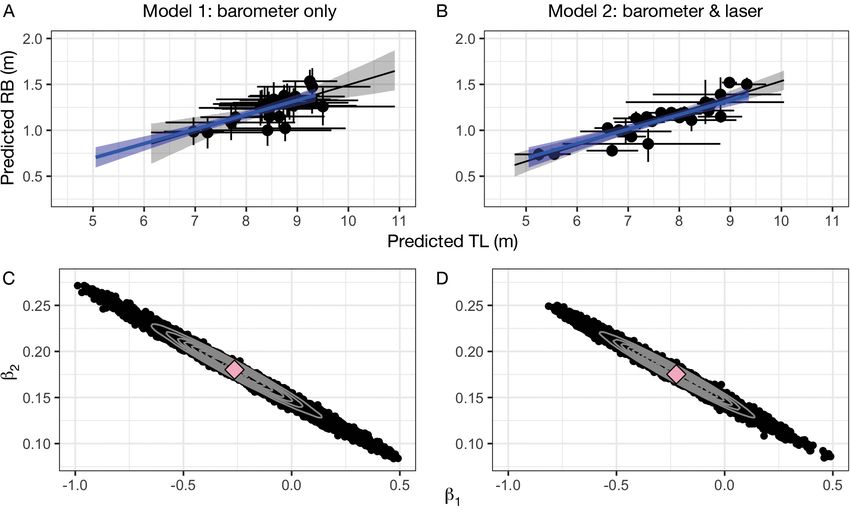
3.2.3. Ecological Scenario 2
We used the Bayesian uncertainty model to estimate
the population-level morphological relationship be-
tween RB and TL for Antarctic minke whales (n = 27)
when using altitude from only a barometer (Model 1)
compared to from both a barometer and laser altime-
ter (Model 2). Linear regression confirmed a linear re-
lationship between empirical RB and TL estimates
(r2 = 0.73, p < 0.001). The mean posterior distribution
for the slope parameter (β2) indicates the population-
level ratio between RB and TL. Model 1 predicted a
slightly smaller β2 with much wider uncertainty
(mean ± SD = 0.17 ± 0.045 [95% HPD interval: 0.08,
0.25]) compared to Model 2 (0.18 ± 0.021 [95% HPD:
0.13, 0.22]) (Table 3, Fig. 7). Overall, Model 1 pre-
dicted larger TL measurements with greater uncer-
tainty compared to Model 2 (Fig. S3), resulting in a
larger population-level mean TL value (μTL) for Model
Fig. 4. Example of predicted posterior length distributions 1 (mean = 8.53 ± 0.196 m) compared to Model 2 (7.67 ±
from Models 1 and 2 for the same individual humpback 0.218 m) (Table 3, Fig. 7). Model 2 more reliably cap-
whale. The longer black bars represent the 95% highest tured the population variability in TL, σTL2
, (mean =
posterior density (HPD) intervals, the thicker shorter black
bars represent the 65% HPD interval, and the black dot rep-
1.171 ± 0.383) compared to Model 1 (0.635 ± 0.308)
resents the mean value. The red dashed line represents the (Table 3, Fig. 7). There was also a decrease in the esti-
average length at maturity for humpback whales (11.2 m) mated value and posterior uncertainty in the popula-204 Mar Ecol Prog Ser 673: 193–210, 2021
Fig. 5. Comparison of the predictive length measurements of humpback whales (n = 48) using Model 1 and Model 2. Each
point represents the mean of the predictive posterior length distribution and the lines around each point represent the 95%
highest posterior density (HPD) interval. Each individual is colored by the % probability of being mature, defined as the
proportion of their predictive posterior length distribution that is greater than 11.2 m, the average length of maturity for
humpback whales (represented by the red dashed line) used by Christiansen et al. (2016, 2020a)
tion variability of RB, σRB
2
, in Model 2 (mean = 0.010 ± uncertainty around UAS-derived measurements. We
0.003) compared to Model 1 (0.013 ± 0.005). Altogether, developed this Bayesian statistical model for re-
the regression parameters (β1, β2) had larger uncertainty searchers using a range of UAS platforms containing
in Model 1 compared to Model 2 (Table 3, Fig. 7). different cameras, focal length lenses, and altimeters
(barometer vs. both a barometer and laser altimeter).
We applied this framework to unknown-sized objects
4. DISCUSSION (e.g. whales) that can be used for probabilistic as-
sessments of ecological importance, e.g. determining
4.1. Novelty sexual maturity, or assessing morphological relation-
ships. Our results represent a standardized practice
Here we built off of previous methods for quantify- for reporting measurement uncertainty and facilitat-
ing photogrammetric error (e.g. Christiansen et al. ing collaboration amongst researchers using differ-
2018, Burnett et al. 2019) and present a Bayesian sta- ent UAS platforms and sensors. Importantly, these
tistical framework for predicting photogrammetric results also allow us to better measure and predictBierlich et al.: Predicting photogrammetric uncertainty 205
Fig. 6. Uncertainty decreases with
altitude. The 95% highest poste-
rior density (HPD) interval widths
(the width of the black bars in
Figs. 4 & 5) of the predictive dis-
tribution decreases with increas-
ing altitude for both Model 1 and
Model 2. Each point represents
the difference between the upper
and lower bound of the 95%
credible interval for each meas-
urement
Table 3. Results from Model 1 (barometer only) and Model 2
(barometer and laser altimeter) in ecological Scenario 2 for morphological features critical to understanding life
estimating the population-level morphological relationship history patterns and potential impacts from anthro-
between total body length (TL) and rostrum to blowhole dis- pogenically altered habitats.
tance (RB) for Antarctic minke whales (n = 27). The mean,
standard deviation (SD), and 95% highest posterior density
(HPD) intervals of the posterior distribution are shown for
each parameter: the intercept (β1), slope parameter (β2) 4.2. Laser altimeter reduces measurement
which indicates the population-level ratio between RB and uncertainty
TL, the population-level mean TL value (μTL), and the scale
parameter which quantifies the amount of population-level
2 2 The results of the present study demonstrate that
variability around the mean TL (σTL ) and RB (σRB )
using a laser altimeter for altitude (Scenarios 1 and 2:
Model 2) reduces measurement uncertainty com-
Mean SD 95% HPD interval
pared to only using a barometer (Scenarios 1 and 2:
Lower Upper Width
Model 1). This was also confirmed in the validation
Model 1 study (Table 2; Table S3). While 95% HPD interval
β1 −0.175 0.380 −0.93 0.58 1.51 widths decreased with altitude for both models in
β2 0.166 0.045 0.08 0.25 0.17 Scenario 1, all mean widths for Model 2 were < 2.0 m
μTL 8.531 0.196 8.14 8.91 0.77
σRB
2
0.013 0.005 0.01 0.02 0.01 compared to < 6.8 m for Model 1 (Figs. 4−6). The val-
σTL
2
0.635 0.308 0.15 1.25 1.1 idation study also revealed that while uncertainty is
Model 2 highest when using only a barometer, using only a
β1 −0.223 0.161 −0.54 0.10 0.64 laser altimeter yields similar results to using a barom-
β2 0.175 0.021 0.13 0.22 0.09 eter and laser altimeter, indicating that the laser
μTL 7.670 0.218 7.24 8.10 0.86
altimeter drives the reduction in uncertainty. Thus,
σRB
2
0.010 0.003 0.00 0.02 0.02
σTL
2
1.171 0.383 0.56 1.93 1.37 we recommend that whenever feasible, a laser alti-
meter should be used for recording altitude. We206 Mar Ecol Prog Ser 673: 193–210, 2021
Fig. 7. Comparison of the morphological relationship between total body length (TL) and rostrum to blowhole distance (RB) for
Antarctic minke whales (n = 27) between (A,C) Model 1: barometer only and (B,D) Model 2: barometer and laser altimeter.
The predictive posterior estimates of RB and TL and their 95% highest posterior density (HPD) intervals (as bars) for each indi-
vidual are shown along with the confidence band for the population-level morphological relationship for Model 1 (A) and
Model 2 (B). The standard linear regression between the empirical, or ‘uncorrected’, measurements of RB and TL is repre-
sented by the blue line with confidence bands in both (A) and (B). Posterior samples for regression parameters highlight the
strong posterior correlation between regression parameters, intercept (β1) and slope (β2), for Model 1 (C) and Model 2 (D). The
pink diamond represents the mean population-level morphological relationship for each model: β2 = 0.166 in Model 1 (C) and
β2 = 0.175 in Model 2 (D)
demonstrate how this can be achieved for ‘off-the- interval width (Fig. 6; Table S3) that will best accom-
shelf’ products, such as the DJI P4Pro, with a custom- plish research objectives based on the UAS aircraft,
made housing (https://github.com/marrs-lab/DJI_ camera, focal length lens, altimeter, and expected
PH4_LaserAltimeter). However, because DJI P4Pro length of the target species. For example, to measure
with video displayed lower resolution and wider changes in body condition of a small cetacean, such
variation in uncorrected % error compared to DJI as a harbor porpoise Phocoena phocoena, smaller
P4Pro with still images (Figs. 2 & 3; Table S2), we rec- 95% HPD interval widths will be required compared
ommend using still images instead of video to reduce to measuring a larger species, such as a blue whale,
measurement uncertainty. and the altitude required to achieve this will depend
While the maximum altitude recorded with the on the UAS aircraft, camera, focal length lens, and
laser in the training data varied across platforms whether a laser altimeter is used in addition to a
(Table S2), all platforms obtained a minimum read- barometer.
ing of 62 m (non-nulled). Thus, flying at altitudes Because barometers are susceptible to rapid
below 62 m may help ensure consistent laser altime- changes in pressure unrelated to a shift in aircraft
ter readings to yield tighter uncertainty predictions altitude, e.g. from gusts of wind, temperature, and
when using this particular laser altimeter. If only changes in barometric pressure during flight, in gen-
using a barometer for recording altitude, then flying eral they have been noted to have poor accuracy
at altitudes greater than 30 m may help reduce the (Sabatini & Genovese 2014) and problems with drift
risk of obtaining measurements with larger uncer- and delay. These problems are more severe with
tainty (Fig. 6; Table S3). Researchers should thus low-cost sensors commonly found on small UAS (Wei
consider collecting data at altitudes that will yield an et al. 2016). Barometric altimeters convert changes
appropriate GSD (i.e. Eq. 1, Fig. 1) and 95% HPD in aerostatic pressure, the difference between theBierlich et al.: Predicting photogrammetric uncertainty 207
atmospheric pressure at a given altitude and the quality in terms of measurability (a flat object float-
pressure set as the zero point, to altitude measure- ing at the surface). Future studies should further
ment (Jan et al. 2008). Variations in temperature and examine the potential for bias introduced when ana-
humidity can impact the aerostatic pressure, and lysts have to choose which images to measure. This
thus the recorded altitude (m) (Bao et al. 2017). These would likely have little influence in the present study,
factors may be particularly influential when flying but could have an effect when selecting images of
over water and may have contributed to the greater whales with larger variation in image quality, such as
predicted uncertainty, especially at lower altitudes glare, refraction, water visibility, and different body
(Fig. 6). Jech et al. (2020) noted differences in barom- orientations (e.g. such as straight, fluke-down, etc.)
eter accuracies compared to Durban et al. (2015, and depths, as shown by Christiansen et al. (2018).
2016), despite using the same UAS platform (APH- The Bayesian framework allows for straightforward
22), that were likely influenced by differences in integration of additional covariates to the model for
temperature. Jan et al. (2008) highlighted how a nor- studies with length predictions that are more heavily
mal procedure for airplanes before arrival at a desti- influenced by different analysts, image quality, and
nation is to adjust the onboard barometer to local repeated measurements of individuals in different
barometric pressure provided by air traffic control. body orientations.
These studies suggest that UAS flown in different
environments may be susceptible to different levels
of barometric error. 4.4. Interpreting predicted measurements
Model 2 in Scenario 1 also displayed greater 95%
HPD interval widths at lower altitudes, though not 4.4.1. Ecological Scenario 1
nearly as wide as Model 1 (Fig. 6). The LightWare
user manual states an accuracy of ± 0.1 m on a 70% Overall, measurements using only the barometer
reflective target at 20°C (LightWare Optoelectronics (Model 1) had larger mean predicted length posterior
2018), so perhaps a combination of temperature and distributions compared to using the barometer and
a less reflective surface at lower altitudes caused this laser altimeter (Model 2). Lengths are a common
increased uncertainty. We recommend that future metric used to classify organisms into demographic
studies record environmental data on each UAS units, such as sexual maturity (i.e. Christiansen et al.
flight to further explore how different oceanic envi- 2016, 2020a, Lemos et al. 2020) and to determine
ronments influence barometric and laser accuracy. population-level impacts of stressors on growth (Stew-
This may be particularly important for studies com- art et al. 2021). Figs. 4 & 5 demonstrate the impor-
paring migrating populations with foraging and tance of including uncertainty around a measure-
breeding grounds in polar vs. tropical regions. ment in these types of analyses, as the conclusion for
It is important to note that the training data used in maturity classification changes depending on which
both models were collected in a much warmer cli- altimeter is used. Several measurements could be
mate compared to the testing data (North Carolina classified differently, and Fig. 4 provides an example
vs. Western Antarctic Peninsula). Future studies of an individual that would be classified as immature
should also record location and date of the training if using the laser and barometer, but as mature ani-
data to see how changes in environment influences mals if using only the barometer (Fig. 4).
measurement predictions. An advantage of the By generating posterior distributions around meas-
Bayesian framework is that it allows for the integra- urements in these types of analyses, the probability
tion of new training data. Thus, researchers working that an animal exceeds a specific length can be com-
in different environments or in similar places at dif- puted to assist in classification and allow ages to be
ferent times of the year can collect, share, and update discussed and studied under uncertainty. For exam-
training data to further improve predictive distribu- ple, classification decisions can incorporate uncer-
tions for future work. tainty through rules, as this present study classified
individuals as sexually mature if 50% of their predic-
tive distribution was >11.2 m. In studies with greater
4.3. Bias uncertainty around each measurement (i.e. only
using a barometer), stricter classification rules can be
No measurement bias was observed across the 3 applied, such as ‘individuals were classified as sexu-
different analysts, but these images were all pre- ally mature if 80% of their predictive distribution
selected by a single analyst and were all of high was >11.2 m’. This further demonstrates the advan-208 Mar Ecol Prog Ser 673: 193–210, 2021
tages of using a Bayesian approach to predict uncer- during estimation. This framework also allows
tainty, where a frequentist approach is limited by repeated observations of the same lengths to be
standard deviations and confidence intervals, which directly incorporated, rather than being manually
may be less accurate and precise. averaged or otherwise summarized before analysis,
and incorporates altitude measurements from multi-
ple altimeters (barometer and laser).
4.4.2. Ecological Scenario 2 The present study provides a robust method for
predicting photogrammetric measurement uncer-
As in Scenario 1, Model 1 had larger mean pre- tainty specific across UAS platforms. This approach
dicted TL posterior distributions with greater uncer- will help researchers set protocols to minimize meas-
tainty compared to Model 2 (Fig. S3). This led to a urement errors during data collection to yield scien-
larger population-level mean TL (μTL) for Model 1 tifically robust conclusions through an analytical
compared to Model 2 (Table 3, Fig. 7). Because the workflow. Standard frameworks like the one pre-
laser altimeter provides more precise and informa- sented here can facilitate collaboration amongst re-
tive measurements than the barometer, Model 2 bet- searchers using different UAS platforms to pool re-
ter captures the variability in the population-level TL sources for comparative studies using past and future
2
measurements (σTL ) compared to Model 1 (Table 3, photogrammetric data to better monitor species and
Fig. 7). This is evident in Fig. 7A,B, where Model 1 populations.
measurements are larger, have greater uncertainty,
are more closely clustered together, and are shifted Data availability. The data and uncertainty model code can
to the right and up from the empirical relationship be found at the Duke University Research Data Repository
(https://doi.org/10.7924/r4sj1jj6s), and instructions for DJI
between RB and TL (blue line) compared to Model 2.
Phantom 4 Pro laser altimeter installation can be found at
Since RB is modeled as a dependent variable relative https://github.com/marrs-lab/DJI_PH4_LaserAltimeter.
to TL, σRB2
models the deviation from the linear rela-
tionship between RB and TL. The estimated σRB 2
value Acknowledgements. We thank Clara Bird and Allison Duprey
is smaller for Model 2 compared to Model 1, and with for assistance in data collection/management; the Duke
less uncertainty (Table 3), which yields the narrower University Marine Lab for project support; and Dr. Andrew
Read for project design and manuscript feedback. Antarctic
model-based confidence bands (grey shading) in humpback whale imagery was collected as part of National
Fig. 7A,B. Science Foundation Office of Polar Programs Grants 1643877
Overall, the regression parameters (β1, β2) had and 1440435 to A.S.F. under NMFS permits 14809 and
greater uncertainty in Model 1 compared to Model 2 23095, ACA Permits 2015-011 and 2016-024, UCSC IACUC
Friea1706.
(Table 3, Fig. 7). The mean population-level morpho-
logical relationship between RB and TL of Antarctic
LITERATURE CITED
minke whales was smaller with much greater uncer-
tainty for Model 1 compared to Model 2 (Table 3, Arnold SJ (1983) Morphology, performance and fitness. Am
Fig. 7). This further highlights the importance of using Zool 23:347−361
a laser altimeter when estimating morphological re- Arona L, Dale J, Heaslip SG, Hammill MO, Johnston DW
(2018) Assessing the disturbance potential of small unoc-
lationships from UAS-based imagery. Morphological cupied aircraft systems (UAS) on gray seals (Halichoerus
relationships pertaining to the skull are commonly grypus) at breeding colonies in Nova Scotia, Canada.
used for distinguishing species (Leslie et al. 2020), PeerJ 6:e4467
tracking ontological growth (Christiansen et al. 2016), Austin PC, Brunner LJ, Hux JE (2002) Bayeswatch: an over-
view of Bayesian statistics. J Eval Clin Pract 8:277−286
and estimating TL when direct measurements of TL
Bao X, Xiong Z, Sheng S, Dai Y, Bao S, Liu J (2017) Baro-
are not obtainable (Ratnaswamy & Winn 1993, Fearn- meter measurement error modeling and correction
bach et al. 2018, Groskreutz et al. 2019). The Bayesian for UAH altitude tracking. In: 29th Chinese Control
framework we present here demonstrates how mor- And Decision Conference (CCDC), Chongqing, China.
IEEE, p 3166−3171. https://doi.org/10.1109/CCDC.2017.
phological relationships are simultaneously esti-
7979052
mated with photographically derived measurements, Best PB, Rüther H (1992) Aerial photogrammetry of southern
rather than in 2 stages, in which physical measure- right whales, Eubalaena australis. J Zool (Lond) 228:
ments are first extracted from photographs and then 595−614
used to estimate morphological relationship. This Burnett JD, Lemos L, Barlow D, Wing MG, Chandler T, Tor-
res LG (2019) Estimating morphometric attributes of
hierarchical Bayesian framework naturally allows baleen whales with photogrammetry from small UASs: a
complex correlations and dependencies between the case study with blue and gray whales. Mar Mamm Sci
measurement error parameters to be accounted for 35:108−139You can also read