Analyze the Impact of Healthy Behavior on Weight Change with a Mathematical Model using the Harris-Benedict Equations

Analyze the Impact of Healthy Behavior on Weight
Change with a Mathematical Model using the
Harris-Benedict Equations
AYAN CHATTERJEE (  ayan.chatterjee@uia.no )
 UiA: Universitetet i Agder https://orcid.org/0000-0003-0407-7702
Ram Bajpai
 Keele University
Martin W. Gerdes
 UiA: Universitetet i Agder

Research Article

Keywords: Mathematical Model, Obesity, Healthy Behavior, Weight loss, Harris-Benedict equations,
Optimization, Health eCoach

Posted Date: June 3rd, 2021

DOI: https://doi.org/10.21203/rs.3.rs-584141/v1

License:   This work is licensed under a Creative Commons Attribution 4.0 International License.
Read Full License

Analyze the Impact of Healthy Behavior on Weight Change with
 a Mathematical Model using the Harris-Benedict Equations
 Ayan Chatterjee1*, Ram Bajpai2, and Martin Gerdes1
 1Department of Information and Communication Technology, Centre for e-Health, University of
 Agder, Norway, email: {ayan.chatterjee, martin.gerdes}@uia.no
 2School of Medicine, Keele University, Staffordshire, UK ST5 5BG, email: r.bajpai@keele.ac.uk

*Corresponding Author:
Ayan Chatterjee Ph.D. Research Scholar
University of Agder,
Department for Information and Communication Technologies (ICT), Centre for e-Health
Jon Lilletuns Vei 9, Grimstad, Norway,
Office: N03 031
Email: ayan.chatterjee@uia.no,
Phone: +47 3723 3812,
Mobile: +47 9471 9372

Abstract
Background: Lifestyle diseases are the leading cause of death worldwide. The gradual
increase of negative behavior in humans because of physical inactivity, unhealthy habit, and
improper nutrition expedites the growth of lifestyle diseases. Proper lifestyle management
in the obesity context may help to reach personal weight goal or maintain a normal weight
range with optimization of health behaviors (physical activity, diet, and habits).
Objective: In this study, we develop a mathematical model to analyze the impact of regular
physical activity, a proper diet, and healthy habits on weight change, targeting obesity as a
study case. Followed by, we design an algorithm to verify our proposed model with simulated
data and compare it with related proven models based on the defined constrains.
Methods: We proposed a weight-change mathematical model as a function of activity, habit,
and nutrition with the first law of thermodynamics, basal metabolic rate (BMR), total daily
energy expenditure (TDEE), and body-mass-index (BMI) to establish a relationship between
health behavior and weight change. Followed by, we verify the model with simulated data
and compared it with related established models. In this study, we have used revised Harris-
Benedict equations (HB) for BMR and TDEE calculation.
Results: The proposed mathematical model showed a strong relationship between health
behavior and weight change. We verified the mathematical model with a proposed algorithm
using simulated data with defined constraints. The adoption of BMR and TDEE calculation
following revised Harris-Benedict equations has beaten the classical Wishnofsky’s rule (3500
cal. ≈ 1 lb.), and the models proposed by Toumasis et al., Azzeh et. Al., and Mickens et. al. with
a standard deviation of ±1.829, ±2.006, ±1.85, and ±1.80, respectively.
Conclusions: This study helped us to understand the impact of healthy behavior on weight
change with mathematical implications and the importance of a healthy lifestyle. As a future
research scope, we wish to use this model in a health eCoach system to generate personalized
lifestyle recommendations to optimize health behaviors to accomplish personal weight goals.

Keywords: Mathematical Model; Obesity; Healthy Behavior; Weight loss; Harris-Benedict
equations; Optimization; Health eCoach.

 1

Contributions to the literature
 • Research has shown that obesity and overweight are strongly linked to a gradual
 growth of negative behavior in humans (e.g., physical inactivity, unhealthy habits, and
 improper nutrition). Appropriate lifestyle management may help to achieve personal
 weight goals or maintain a normal weight range by optimizing healthy behaviors.

 • Scientific evidence has bolstered the relation between weight change and body-
 energy imbalance by following the first-order rule of thermodynamics. Weight
 change is not a straightforward process. It involves multiple biological factors and
 complex biochemical processes.

 • Research has shown the existence of different weight-change mathematical models.
 However, there is no evidence on how they can certainly be applied in a digital health
 management program to promote a healthy lifestyle (e.g., health eCoaching).

 • Therefore, we propose a simple mathematical model based on first-order derivatives
 to derive a strong relationship between health behavior and weight change. The
 verification of the model with simulated data was performed with another proposed
 algorithm. Furthermore, we elaborate how the model and algorithm can be used in a
 health digital recommender system for optimizing health behaviors.

Introduction
Overview
Globalization, rapid urbanization, and sedentary lifestyle have promoted negative health
behaviors globally, affecting individuals from different financial backgrounds [1-4]. The
major risk factors behind a sedentary lifestyle are - inadequate dietary intake, unhealthy
habits, and physical inactivity [1,2,5,6]. The curse of a sedentary lifestyle can be - obesity,
increased glycemic response, high blood pressure (BP), increased blood cholesterol, and
depression [1,2,5]. Obesity is accountable for other lifestyle diseases, such as cardiovascular
disease (CVDs), chronic obstructive pulmonary disease (COPD), cancer, type II diabetes, and
hypertension [1,2,5,6]. Lifestyle diseases are the most leading cause of death in the world [1-
4]. The primary likelihood of mortality is between ages 30 and 70 years, and by 2030, eight
of the ten leading causes of death will be related to their risk status rather than gender [7].
The development of healthy behaviors may prevent the increased likelihood of lifestyle
diseases and premature death worldwide [1,7-12]. From 1980 to 2008, The incidence of
obesity has almost doubled. In 2008, 1.5 billion adults had a body mass index (BMI) above
25, and about 500 million of them were considered obese [13]. In 2016, 1.9 billion+ adults
over 18 and 340 million+ children and adolescents aged 5-19 were overweight. Obesity was
responsible for 8% (4.7 million) of global death worldwide in 2017 [14]. Most of the world’s
population lives in countries where overweight and obesity cause more deaths than
underweight [13-16]. Obesity does not grow overnight. It develops over time because of poor
diet, lifestyle factors, physical inactivity, genetics, family history, race, ethnicity, sex, family
habits, culture, social environment, and medical background [17-19]. Therefore, a healthy
lifestyle is essential to keep up, accomplish, or regain good health and prevent sickness.
Healthy behavior includes - regular physical exercise (to stay active, adequate sleep), a
nutritious diet (adhere to core foods such as fruits, vegetables, and whole grains), and healthy
habits (no consumption of alcohol and tobacco, and positive attitude) [1,7-12]. Obesity and
overweight are major lifestyle diseases, occur because of body-energy imbalance [11,12,20].

 2

The excess amount of energy gets stored as a mass in the body and is termed as “weight gain”
[11,12,20]. Scientific proofs emphasize that a proper dietary habit is essential to a healthy,
sustainable, and quality lifestyle. A healthy nutritional pattern helps individuals to keep up
adequate body weight [21,24]. Moreover, regular physical activities and keeping up a healthy
habit expedite weight change in a positive direction [21,34]. Hall et al. [35,36] stated that
getting thinner slows down an individual's metabolism. If individuals need to shed ten
pounds of weight at the end of the year, they need to cut a hundred calories per day either by
consuming fewer calories or more workout [35,36].

Background
Early weight loss (i.e., the first few weeks) tends to have a lower energy content than weight
losses on subsequent weeks [37]. Forbes [38] first expressed the statistical model of the
weight loss cycle, which revealed that the composition of long-term weight loss differs
between thin and obese women. The result raised doubts on the research of Grande [39],
performed in a group of average weight men. In addition, several previous weight loss studies
conducted on obese women responded differently to male interventions [37-39], suggested
that men lose more lean mass and less fat than women during periods of energy imbalance.
First, Forbes and later Hall [40,41] proposed the correlation between the proportion of
weight loss with fat-free mass (FFM) and baseline fat mass (BFM). Forbes [40] used cross-
sectional body composition data to explain the non-linear observational relationship
between FFM and FM and concluded that the longitudinal change of body composition might
be defined by the displacement along the cross-sectional curve theoretically. According to the
study of Heymsfield et al. [42] on the Keel research data set, the weight change is not
"constant" following Wishnofsky's law [22,23] but is essentially "dynamic". Hall et al. [43,44]
proposed simple dynamic model estimates (for example, when the weight reaches a new
steady-state, a change in energy intake of 10 kcal/day will result in a weight change of 1
pound). In addition, Heymsfield et al. [42] showed that, at least for those with similar BMI,
the energy content of weight loss varies significantly between men and women.

Obesity is considered as a metabolic syndrome (MetS) [45]. Fat-mass index (FMI) and body
mass index (BMI) are metrics used to diagnose obesity [46]. Samadi et al. [47] reported that
FMI is more accurate in terms of sensitivity and specificity than BMI. The BMI is the most
used method for assessing overweight and obesity. However, BMI does not always represent
real body fat. It can be calculated by calculating body fat or BF (based on age, weight, height,
neck, and waist circumference) and fat-free mass (based on height, weight, and BF%). Despite
BMI or BF%, higher FMI levels tend to correlate with the existence of MetS. Fat-mass (FM)
and FMI are closely related to body composition [45]. Bioelectrical Impedance Analysis (BIA)
[45] is the most superficial, most repeatable, and lowest cost tool for determining BF% in
clinical practice. It has high precision and is excellent in comparison with the dual-energy X-
ray absorption method (DXA). BF% accuracy is affected by height and cannot be measured
separately from the fat-free mass (FFM). The fat-free-mass index (FFMI) [45] is an alternative
to the BMI, which considers a person's muscle mass. FFMI measures the total amount of lean
muscle mass in the body. It may also be able to predict how much muscle the body will gain,
according to studies. It is a good indicator for people trying to lose weight, particularly those
who are doing strength training to build muscle and lose fat. FFMI is particularly helpful to
severe bodybuilders [45]. In contrast to women, men have less body fat, more muscle mass,
and higher bone density, according to the National Health Service (NHS) [48]. FFM is
calculated as a function of height, weight, and BF%. If we have more muscle than the average
person, it is difficult to tell the difference between fat and muscle. According to a 2003 study
published in Nutrition [48,49], BMI alone cannot provide information about fat-free mass or

 3

fat mass to body weight. Kim et al. [4] claimed waist-to-height ratio as a better tool than BMI
and waist circumference to screen obesity and overweight, which requires more validation.

Weight-maintenance calorie or total daily energy expenditure (TDEE) is the total necessary
calorie consumption per day when individuals are moderately active [64]. TDEE depends on
basal metabolic rate (BMR). BMR can be measured based on the FFM value (lean mass and
bone mineral content) using the Cunningham [82] or Harris Benedict’s equations [64].

Motivation
We have considered human behavior as a function of activity, diet, and habit in our proposed
mathematical model. We have applied modified Harris-Benedict’s equations [64] with
physical activity level or PAL (“α”) for the TDEE calculation [50]. The “α” value can be
assessed with wearable activity devices (e.g., Fitbit, MOX2), daily. For general population, BMI
calculation is very straightforward based on height and weight only. Therefore, we have used
the BMI metric for obesity categorization as a substitute of FFMI. Genetics, FM, FFM, waist-
hip ratio and waist measurement are beyond the scope of this study. We focused only on
obesity assessment in the general healthy adults rather than special categories, such as
children, the elderly, bodybuilders, disabled, and people consuming steroids. We will focus
TDEE calculation on a more granular level based on weight change dynamics, metabolic
adaptation, LBM, FM, and FFM in our future studies.

The aim of this study can be divided into the following two sections –
(a.) to develop a mathematical model to establish a relationship between health behavior
(activity, diet, and habits) and weight change; and
(b.) model verification with simulated datasets based on a proposed and implemented
algorithm.

Existing Weight-Change Mathematical Models
Different research groups proposed different methods to model human weight change over
time. In this study, we included core weight-change mathematical models related to energy
expenditure, and excluded models which are primarily focused on nutrition assessment (i.e.,
macronutrient flux balance, nutrient level), genetics, and complex biochemical processes
(e.g., lipolysis, ketone oxidation, proteolysis, glycerol 3-Phosphate production, glycerol
gluconeogenesis, gluconeogenesis from amino acids, macronutrient oxidation, lipogenesis,
carbohydrate and protein perturbation, and respiratory gas exchange). Wishnofsky rule's
[22,23] fundamental analysis states that reduced energy consumption decreases the
enforced energy deficit and delays weight loss when people lose weight. On the first day of
diet, reducing consumption by 500 kcal results in an energy deficit of 500 kcal, but the extent
of this deficit and the weight loss decreases dramatically with time. However, the biochemical
processes in the body are much more complex [22,23]. The self-limiting principles of steady
weight loss are as follows - the loss of energetically active tissue, metabolic adaptations, and
a lower cost of weight-related energy expenditure [22,23]. According to the second
evaluation of Wishnofsky's law [22,23], the composition of voluntary diet–induced weight
loss is based on the subject's initial body composition. Obese people lose mostly energy-dense
fat because they have a negative energy balance, while lean people lose a lot of fat-free mass
with a low energy content (FFM). Obese subjects must decrease their energy consumption
more than lean subjects to lose one pound while having a "healthier" composition of weight
loss. This "early" weight reduction effect, which is frequently dismissed as unimportant, will
typically bring down the energy content of weight loss well below Wishnofsky's law [22,23].
Forbes, in 1970, first conceptualized a mathematical model related to weight change. He used

 4

cross-sectional body composition data to explain an observational, non-linear relationship
between FFM and FM, speculating that longitudinal changes in body composition were
defined by displacement along the cross-sectional curve [40]. The empirical function of their
model can be expressed as follows –

 FFM = f(FM) = 10.4 + + 14.2
where FM = initial body fat and both FM and FFM are in Kilogram (Kg.)

According to Forbes [40], shift along the cross-sectional curve defines longitudinal changes
in body composition. The following equation was derived for infinitesimal body weight (BW)
shifts (dBW). Therefore, Forbes' theory predicted that FFM's contribution to an infinitesimal
weight shift was exclusively dependent on the FM.

 10.4
 =
 10.4 + 

Hall extended Forbes’s theory [40] to explain macroscopic weight changes. In addition to the
initial FM, the new equation predicts that the composition of weight change is determined by
both the direction and magnitude of the weight change. Experimental data from underfeeding
and overfeeding humans were compared to explain the connection between Forbes' theory
and the P-ratio, an alternative representation of body composition change that assumes the
existence of an energy partitioning parameter. The P-ratio is a measure of how much of an
energy imbalance can be explained by changes in the body's protein reserves. Initially, the P-
ratio was thought to be a constant for everyone. According to the new version of Forbes'
theory, the P-ratio is affected by the initial body composition as well as the direction and
magnitude of weight loss [40].

 ∆ ⁄∆ 
 =
 (∆ ⁄∆ ) + (1 − ∆ ⁄∆ )
 where α = 9.05 represents the ratio of the energy densities of FM to FFM.

Kien et al. [50] performed a study on 26 healthy, nonobese young adults for 28-days and
came up with an improved prediction of TDEE in terms of resting energy expenditure (REE).
To maintain a constant body weight, energy intake was adjusted. FFM and FM were measured
using dual-energy X-ray absorptiometry before and after the study period, and TDEE was
calculated using the change (after and before) in body energy (BE) and observed energy
intake (EI): TDEE = EI - ΔBE. A TDEE estimate based on the Harris-Benedict equation (TDEE
= 1.6 * REE) was examined. The measurements suggest the following estimation of TDEE –

 = 1.60 − 1.86 ∗ 
 = (21.2 ∗ ) + 415

Toumasis et al. [21] developed a mathematical diet model in 2004 to describe the
relationship between weight change and calorie expense. They considered consumed energy
as “C” and expensed energy as “40B” (where, 40 is the mean of 35 and 45 that signifies average
calories/kg./day depending on factors, such as age, sex, metabolic rate). Their proposed
mathematical relationship can be written as follows -
 
 = A (C - 40B),
 
where B = current body weight, and A = energy constant

 5

Their resultant model for weight change with calorie can be written as below:

 ( ) = + � 0 − � −0.0052 ,
 40 40
where B (0) = B0 is the initial weight, t = days

In Toumasis’s model, neither dietary nor habit components were considered, and the daily
rate of energy expenditure (a = 40 Cal/kg/day) was obtained from primitive techniques.
Azzeh et al. [54] improved the model proposed by Toumasis et al., in 2011, with an additional
component, such as exercise. They conducted a study on twenty students who walked on a
treadmill for thirty min., at a fixed speed of 3.2 km./hr., in a varying temperature range
between 200 to 250 celsius (C). The trial's principal objective was to establish a connection
among weight and the measure of energy consumed per individual because of activity. They
upgraded the model as follows:
 
 = ( − ),
 
where B = current body weight, A = energy constant, and b = a+7.876.

They observed the ratio of energy burned due to the treadmill activity to body weight, on
average, is 7.876 (KJ/kg)/day. They observed better weight-loss than the previous model
with exercise component. Their resultant model for weight change can be written as:

 ( ) = + � 0 − � − ,
 
where B (0) = B0 is the initial weight, t = days.

Azzeh’s proposed model was not entirely accurate due to the selection of a small sample size.
No habit components were considered in the model, and the daily rate of energy expenditure
(a = 40 Cal/kg/day) was obtained from primitive techniques. They further proposed to
improve the model with ambient temperature as formulated below, where the factor “b”
depends on heat and mass transfer, and ambient temperature has an impact on body
thermoregulation, and metabolic rate:

 ( ) = [ − � + ( )� ],
where F(T) function depends on ambient temperature.

Mickens et al. [55] proposed a mathematical model on the dieting process, which is non-
linear, and based on first-order differential calculus. They determined all the features of the
model with linear stability analysis and phase-space techniques. Their developed model can
be formulated as below:

 = ( ) − ( ) − ( )
 
where F(t) = intake function, E(t) = measures of physical activity, F(t)-E(t) = λ > 0, and M(W) =
metabolism function ~ Wα and α ≈ 0.7
 ( ) 3
 Therefore, ( ) = = 4 ,
 1+ 1− 
where 0< α 0.

Neither activity nor habit components were considered in the Mickens’s model. Horgan et
al. [56] used a stochastic process to model weight changes and explained its behavior as an

 6

autoregressive process. According to their model, if intake and activity maintain a constant
mean, bodyweight will stay within a few percent of a fixed point. It is easier to see that activity
levels will maintain natural stability because they have a lower bound, no matter how
sedentary one becomes. Aldila et al. [57] proposed a state change mathematical model for
obesity on a closed population to demonstrate that the intervention program with sound life
mission and restoration has an altogether diminished number of obese individuals. They
considered factors such as natural recruitment rate (/day), natural mortality rate (/day),
interaction coefficient (/day), infection rate because of bad life habit (/day), natural recovery
rate from overweight to healthy comp (/day), total individuals, health recruitment rate, life
campaign rate, and treatment rate for the obese population. Their proposed model requires
the inclusion of social interaction rate, demographic classification, and personalization. The
proposed model suffers from model validation with social interaction, activity, and age.
J´odar et al. [58] presented a 3–5-year-old childhood obesity model to contemplate obesity
in the Spanish area of Valencia. They considered the following factors in their non-linear
system of first-order differential equations – transmission rate due to social pressure for BFS
(bakery, fried meals, and sweet beverages) consumption, BFS consumption, time, interaction,
and diet. The mathematical model derived the increasing trend of child obesity in Valencia
due to the frequent consumption of BFS. Their considered parameters in the model are
constant over long period of time and suffers from model validation with physical activity. A
similar study was performed at Valencia on 24-65 years old residents by Santonja et al. [59].
They proposed a mathematical model to foresee the frequency of abundance weight in the
population in the forthcoming years. They found that a sedentary lifestyle and nutritional
habits are behind the reason of weight increase in the society. Their proposed mathematical
model considered factors such as lifestyle, time, weight transition, diet, and social interaction.
However, their considered factors were constant over long period of time. Thomas et al. [60]
proposed a mathematical model for non-diabetic patient, with first-order differential calculus
related to weight change with following key factors - resting metabolic rate (RMR), non-
exercise activity thermogenesis, and dietary induced thermogenesis. Their model can be
represented based on the first-order law of thermodynamics. However, the model suffers
from accurate measurement of energy expenditures based on the considered parameters:

 = − ,
where, R = rate of energy stored or lost, I = rate of ingested energy, and E = rate of expended energy.
Therefore,
 
 = + � � + ,
 
where, G = time average constant, FFM(t) = fat free mass = 10.4 ln(F(t)) + 14.2, F(t) = fat mass, and
initial condition: F (0) = F0 > 0
 = + + + ,
Provided,
 DIT = energy involved in processing food = βI, where β is constant
 PA = rate of weight bearing exercise = mW = m (FFM(t) + F(t)), where W = body weight
 
 RMR = rate of energy required to sustain life = (1 − ) � − � 0 + ��, where, A =
 365
age, A0 = age at time “t” = 0, ≤ a ≤ 1, aM = 293, aF = 248, pM = 0.4330, pF = 0.4356, yM = 5.92, yF = 5.09, W
= body mass
 NEAT = thermogenesis that comes with physical exercises other than volitional exercise =
 
 ( + + ) + , where, r =
1− 

There are no mathematical models that are fully accurate. Based on the assumed restrictions,
each of them has their merits and demerits as specified. However, the knowledge obtained

 7

after studying different weight-change models helps us to formulate our projected
mathematical model to analyze the correlation between healthy behavior (activity, diet, and
habit) and weight change. This study enhances mathematical model proposed by Toumasis et
al., with the inclusion of metabolism (BMR), TDEE, activity level (α) (calculated with revised
HB equations), healthy diet, and healthy habit. The activity level (α) helps to calculate TDEE
with the BMR following revised HB equations [63, 64, 69, 78]. Furthermore, we have
demonstrated how weight change can be represented as a function of activity, diet, and habit.
Our proposed model aims at showing how the optimization of health behaviors can help to
accomplish weight change goals! An algorithm has been proposed for the verification of the
proposed model. Our target is to improvise both the model and algorithm in the future to use
them in a health eCoach recommender system for healthy lifestyle promotion with the
generation of tailored lifestyle recommendations. We compared our proposed model with
the related weight change and body-energy imbalance models proposed by Wishnofsky,
Toumasis et. al., Azzeh et. al., and Mickens et. al. (see Table 1) with simulated data for
performance evaluation.

Methods
This section is distributed among the following three subsections – (a.) relevant formulas for
this study, (b.) mathematical model development, and (c.) algorithm for model evaluation.

Relevant Formulas
In 1918 and 1919, the original Harris–Benedict equations were written [64]. Roza and Shizgal
updated the Harris–Benedict equations in 1984, and they found 95% of confidence range for
men is 213.0 kcal/day and 201.0 kcal/day for women. The equations were updated once
more by Mifflin and St Jeor in 1990 [64] to reduce the root mean square error (RMSE). In this
study, we have used the latest version of HB equations as mentioned below -

For Men in metric:
BMR = (10 * weight in kg.) + (6.25 * height in cm.) - (5 * age in yrs.) + 5 ------- (eq. 1)
For Women in metric:
BMR = (10 * weight in kg.) + (6.25 * height in cm.) - (5 * age in yrs.) - 161 ------- (eq. 2)

Apart from the HB equations, BMR can be measured with Katch McArdle Formula based on
lean body mass (LBM) [66,67]. Calorie estimation considering lean body mass (LBM) gives
the most exact result of energy use; however, even without LBM, we can get a sensibly close
estimate. Lean body mass (LBM), pregnancy, bodybuilding, heredity, and child obesity are
beyond this paper's scope for BMR calculation. Therefore, in our proposed weight-change
mathematical model, we reused Harris-Benedict’s linear equation for BMR representation, as
follows:

BMR = C1 + C2 * weight + C3 * height – C4 * Age,
where, C1, C2, C3, C4 are numeric constants. Their values can be taken from (eq. 1), and (eq. 2) based on
the gender. (eq. 3)

After BMR calculation, we calculated TDEE by multiplying the BMR value by activity level as
shown below [63,69]:

TDEE (Sedentary) = BMR * 1.2 (little or no exercise, desk job). [α=1.2] (eq. 4)
TDEE (Lightly active) = BMR * 1.375 (light exercise/ sports 1-3 days/week). [α=1.375] (eq. 5)
TDEE (Moderately active) = BMR * 1.55 (moderate exercise / sports 3-5 days/week). [α=1.55] (eq. 6)

 8

TDEE (Very active) = BMR * 1.725 (hard exercise every day, / sports 6-7 days/week). [α=1.725] (eq.
7)
TDEE (Extra active) = BMR * 1.9 (hard exercise 2 or more times per day, or training for marathon, or
triathlon.) [α=1.9] (eq. 8)
Therefore, TDEE can be represented as: TDEE = BMR * C5, where C5 is the activity multiplier constant
and its value > 0. (eq. 9)

Body-mass-index (BMI) is another critical health factor responsible for assessing individuals’
nutritional status and classification of individuals in the following categories – underweight,
normal weight, overweight, and obese, in a very simple approach, based on their weight and
height [70]:

BMI = (weight / height2) * 703,
where, weight is in pounds (lb.), and height is in inches (inch.). (eq. 10) [SI unit: Kg/m2]

BMI does not change with age or gender. It is certainly not a direct estimation and is just
utilized as a screening tool and subsequently, not considered an in-depth analytic test. There
are additionally a few constraints to this estimation. Since BMI uses just tallness and weight,
it does not represent individuals who might be a lower in average physique yet better than
expected bulky person, such as bodybuilders. Such constraints are beyond this paper's scope.
In this study, for measuring individual’s weight category, we have focused on BMI value. The
BMI constraints are age, gender, height, weight, activity, metabolism, temperature, ethnicity,
muscle mass, and body fat.

Measurement of ideal body weight (IBW) is important for individual weight management. To
verify our proposed model and ideal weight convergence, we followed Miller’s equation [71]:

D. R. Miller Formula (1983):
Male: 56.2 kg + 1.41 kg per inch over 5 feet (eq. 11)
Female: 53.1 kg + 1.36 kg per inch over 5 feet (eq. 12)

Development of the Proposed Mathematical Model
Proper dieting is a habit of eating and drinking in a controlled approach to lose or, sometimes,
increase weight, or in some cases, to normalize the amounts of certain nutrients. Reducing
weight with cutting down daily consumption is a slow process, but it can be accelerated in
combination with regular physical activities. The same is proved in our proposed model. In
overall calculation, we considered temperature as a constant. The model is applicable for
checking variation in limited period weight change with the adoption of healthy habits for
fixed age and height. We wish to use this model in a health eCoach system to generate
personalized lifestyle recommendations to optimize health behaviors to accomplish personal
weight goals. The influence of body weight variability [79, 80] will be added to this model in
the future after a detailed study on a group of trials.
 
 = C*(Y-X) [kg/day] ----- (eq. 13)
 
provided,
 W = current weight,
 Y = Daily calorie intake (assumed fixed here),
 X = Calorie required for daily activity (total daily energy expenditure or TDEE that varies with
 activity level ‘α’ in a direct proportion)
 C=1/7700 calorie [1 kg = 7700 calorie, and 1lb = 3500 Kcal.]
Therefore,

 9

 
 = C*(Y-TDEE) [kg/day] ----- (eq. 14)
 
 TDEE = activity level (α) * BMR ----- (eq. 15) [see: eq. 9]

Note: In remote health monitoring, we can monitor individual activity level with wearable activity
sensor devices and calculate corresponding ‘α’ value.

BMR = C1 + C2*weight + C3*height – C4*Age, where C1, C2, C3, C4 are numeric constants. ----- (see eq. 3,
based on revised Harris-Benedict equations)
Therefore,
BMR = function (weight, height, age) based on Harris-Benedict equations.
For fixed height and age, BMR = function (weight) = C2*weight + K, where K is a constant, and
can be represented as, K = (C1 + C3*height – C4*Age) ----- (eq. 3)

For fixed height and age, above (eq. 33) can be written as:
 
 = C*{Y-(β1+β2*W)},
 
where, β1, β2 are constants and it depends on ‘α’ with direct proportion -------- (eq. 16)
and,
 β1 = α * K and β2 = α * C2

Let, Y = (Y1 + Y2), where Y1 = Calorie consumption through regular dietary intake, and Y2 = Calorie
consumption through unhealthy habits (e.g., alcohol in this context). We hypothesized that an amount
of Y1 and Y2 could reduce fixed calorie intake (Y) with proper diet (Y1) and healthy habit (Y2)
measured in Kcal. Therefore, Y can be expressed as Y = function (Y1, Y2). Our target is to optimize Y2 ≈
0 with a gradual reduction of daily alcohol consumption. As an example, a wine at 12.5 % vol contains
12.5ml of liquor/100ml of wine * 0.8 g/ml = 10g of liquor/100 ml of wine. It can be compared to 1
drinking unit (≈ 10 g) [75]. 10 g. alcohol contains approx. (10*7.1) = 71.1 kcal. We wish to lower daily
or weekly, or monthly alcohol consumption and optimize Y2 ≈ 0 with motivational personalized
lifestyle recommendations. Smoking is excluded from this preliminary model due to the quantification
problem in terms of calories. However, we will further improve this model with a smoking parameter
in the future after a detailed study on a group of trials.

Therefore,
 
 = C*{(Y-β1-Y1-Y2)-β2* W} -------- (eq. 17)
 
Solving the (eq. 17):

 + ∗ 2 ∗ W(t) = ∗ (Y − 1 − 1 − 2 ) -------- (eq. 18)
 
Multiplying by integrating factor ∗ 2 on both sides,

 ∗ 2∗ + ∗ β2∗ ∗ 2∗ W(t) = ∗(Y-β1-Y1-Y2) ∗ 2∗ 
 
Or,

 � ∗ 2∗ W(t)� = [ ∗(Y-β1-Y1-Y2)/(C* β2) ∗ 2∗ ]
 
Or,

 � ∗ 2∗ W(t)� = ((Y-β1-Y1-Y2))/(β2) ∗ 2∗ + 

 10

(Y−β1− 1 − 2 )
At t = 0, = (0) −
 β2

The final weight function at time “t”:

 ( − − − ) ( − − − )
 ( ) =
 
 + � − �
 
 �� ∗ − ---------- (eq. 19)

 ( − − − )
Initially (at t=0), W(t) ≈ W0 = , where Y1=Y2=0 ------------ (eq. 20)
 
From (eq. 39), it is obvious that the weight of an individual changes with physical activity,
proper dietary, and healthy habits, following the below convergence criteria (see Figure 1):

 < , ( ) > 
 
 = �> , ( ) < ------------ (eq. 21)
 
 = , ( ) = 

Note: The denominator β2 depends on activity level (α). According to the (eq. 19), weight loss ∞ β2 (=
α*C2). The sign of Y1, and Y2 in (eq. 18) defines if it is a calorie augmentation (-) or reduction (+). They
are applicable from t>=1.

Figure 1. An ideal weight convergence diagram based on (eq. 21) (at “t” =0, W1>W0>W2>0)
 [X-axis: time in days, and Y-axis: individual weight]

Model Evaluation with Simulated Data and Proposed Algorithm
The proposed model has been evaluated in the following three directions – a. visualization of
tentative weight convergence for a limited number of days (e.g., 30-90 days in this context),
b. comparing the performance of the proposed model with related models as described in
Table 1, under defined settings, and c. calculation of number of days to reach personal ideal
weight goal. In this study, we simulated data for six dummy participants as detailed in Table
2, where participants are created for three weight groups – overweight, underweight, and
normal weight. Their target weight has been determined by ideal body weight as calculated

 11

with (eq. 11) and (eq. 12). In the subsequent section, we describe how the adoption of healthy
behavior influenced weight convergence or maintaining a normal weight range.

The algorithm for model evaluation with dynamic behavior change based on defined rules:

 Algorithm Adult’s weight change goal evaluation with optimization of healthy behaviors
 Step 1: Initialize necessary parameters of all participants in a *.csv file as follows to
 create a simulated environment –
 Example (P-1 on day-0 as explained in (eq. 40)) dataframe: height = 170.18/*present fixed
 height in cm*/, weight = 82/*present weight in Kg*/, age = 33/*present round-off age in
 years*/, gender = “male”, daily_average_alcohol_consumption = 125 /*quantity in ml.*/,
 activity_level = “sedentary”, healthy_diet = “No” /*nature of diet healthy or unhealthy*/, Y1 =
 0 /*initial change in calorie intake due to dietary habit*/, daily_calorie_intake = 3000 /*It is
 “Y” in (eq. 13) in Kcal*/, smoking = “no”, days = 90 /*duration of the experiment*/,
 target_weight = 66.07/*target weight range for convergence based on (eq. 11) and (eq. 12)*/
 Step 2: Calculate BMI for the assessment of body composition and classify each
 participant in one of the following weight group: {underweight, normal weight,
 overweight, obese}
 Step 3: Calculate daily calorie (Y2 in eq. 17) consumption due to individual habit. /*It
 needs to be reduced for healthy habit adoption*/
 Step 4: /*Dynamic change in habit based on the rule*/
 for day = 1 to days do
 Step 4.1: If (present_weight == target_weight) then,
 Y1 = Y2 =0,
 (Y-Y1-Y2) = Y /*No change in calorie input*/
 (Y-X) = (Y-TDEE) = 0 /*No change in activity level*/
 Else if, (present_weight > target_weight) then,
 activity level = select one-level better activity level than the previous
 day’s activity_level from activity_group (if “extra active”, then choose “extra active” only)
 daily_average_alcohol_consumption = select alcohol consumption if
 participant consumes daily alcohol, else 0
 healthy_diet = “Yes”
 Y2 = calculate calorie from daily_average_alcohol_consumption
 Y1 = restricted (-ve) calorie consumption following appropriate
 dietary guidelines
 Update (Y-Y1-Y2), weight, BMR, TDEE /*Y is fixed, but Y1 and Y2 are
 variable. The Y1 and Y2 values can be personalized with health eCoach recommender system
 based on personal weight-loss goal */
 Else
 activity level = select one-level reduced activity level than the
 previous day’s activity_level from activity_group (if “sedentary” or “lightly active”, then choose
 “lightly active” only)
 daily_average_alcohol_consumption = select alcohol consumption if
 participant consumes daily alcohol, else 0
 healthy_diet = “Yes”
 Y2 = calculate calorie from daily_average_alcohol_consumption
 Y1 = augmented (+ve) calorie consumption following appropriate
 dietary guidelines

 12

Update (Y+Y1+Y2), weight, BMR, TDEE /*Y is fixed, but Y1 and Y2 are
 variable. The Y1 and Y2 values can be personalized with health eCoach recommender system
 based on personal weight-gain goal*/
 Step 4.2: Append W(t) in a list, and update BMI value.
 Step 5: Measure body composition based on final BMI value and compare with initial
 value.
 Step 6: Plot the list as weight change (Y-axis) over number of days (X-axis) to visualize
 the trend of weight change of individual participants. The convergence of the graph should
 follow (eq. 21).

Note:
  The worst-case time complexity of the proposed algorithm is O(N2), where N = problem size
 > 0. The proposed algorithm is implemented in Python 3.8.5 with Spyder4 editor in Anaconda
 distribution.
  Behavior change is a slow and complex process. Daily activity, drinking habit, and calorie
 intake from dietary habit cannot be fixed. Therefore, we must consider some randomness in
 their value selection in terms of calorie for real-life situation. Therefore, this algorithm can be
 improved further with real-time, automatic, personalized lifestyle recommendations (with a
 health eCoach system). The weight-convergence will change over days with a modification in
 the assumed values of activity level, calorie input through diet, and habit in the algorithm as
 designed above.
  If individuals need to lose weight, then they need to reduce their calories a day by reducing
 calorie intake or increasing exercise [35,36]. The defined rules and values in the algorithm are
 adjustable based on personalized goals. We assumed a changing value of {-(Y1+Y2)} in the
 range between 100-600 kcal in weight-loss simulation testing. We adopted a dynamic value
 of (Y1+Y2) between 600-1000 kcal in weight-gain simulation testing to augment daily calory
 consumption. However, it must be related to other personalized parameters, such as context,
 activity level, and physical condition. We will add this dynamic feature to our proposed model
 in the future during a detailed study on a group of controlled trials.
  The novelty of using the proposed model and the algorithm in a health eCoach recommender
 system for optimizing health behaviors is conceptualized in Figure 2.
  The codebase for data configuration, algorithm development, and data visualization can be
 downloaded from the GitHub (Digital Appendix 1) for code reproducibility.
  Used libraries in the simulated python environment are described in Table 3.
  The configuration of the system and used software in this study are described in Table 4 and
 Table 5, respectively.

Figure 2: Usefulness of the proposed model and algorithm to optimize health behaviors.

 13

Results
We implemented the algorithm over simulated participants (“P-1” to “P-6”) for a fixed
duration of 30 days, 60 days, and 90 days, consecutively as described in Table 6. Figure 3
depicts how weight change is occurring based on our proposed model for the simulated
participants over a duration of 90 days. Then we compared the weight-loss convergence in
our model with other models proposed by Wishnofsky, Toumasis et al., Azzeh et al., and
Mickens et al. for all the participants over 90-days, and as an example, the result of participant
“P-1” is depicted in Figure 4. We obtained better weight-loss convergence than other models
under provided settings, and it proves that healthy behavior (proper physical activity,
appropriate dietary intake, and healthy habit) has a significant impact on weight-change.
Therefore, adoption of healthy behavior can help weight-loss in obese/overweight.

Figure 3: The weight change with the proposed model for the simulated data over 90 days.

 14

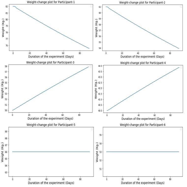
Figure 4: Weight (Kg.) loss of example participant “P-1” for different models over days

 15

X Axis - No. of Days, Y Axis - Weight (Kg.)
 80.99
 80.13 80.4 80.2
 81 80.06 80.01
 79.39 79.6 79.68
 80
 79 78.11 78.2
 77.5 77.52
 78
 76.16
 77 75.51
 76
 75
 74
 73
 72
 Wishnofsky’s Toumasis et al. Azzeh et. al. Mickens et. al. Our Model
 rule

 After 30 days After 60 days After 90 days

 Table 7 demonstrates how long it might take to reach the targeted ideal body weight for
individual participants “P-1” to “P-4” (we exclude “P-5” and “P-6” as they are already at
normal weight range) with our proposed model. The rules for health behavior change in the
algorithm can be made dynamic for personalized recommendation generation to promote a
healthy lifestyle.

Discussion
In this model, we have shown how weight loss/gain can be described as a function of activity,
diet, and habit. FFM-based TDEE calculation does not include activity level and needs
expertise for data capturing. Thus, we followed activity based TDEE calculation following the
revised HB equations which is based on simple parameters with less measurement overhead.
According to this algorithm, the recommendation generation is rule driven. However, it is the
scope of future research to convert it into hybrid (rule driven and data driven). This model
has certain limitations. Quantifying weight-change over time is a complex task because of
multiple influencing factors, as stated in the introductory section. If the FFM knowledge is
unavailable, then the HB, revised HB, or WHO equations are possible alternatives, but their
accuracy on an individual level can be minimal [76]. At an elementary level, the original HB
equations, or their more accurate revised versions (Roza and Shizgal in 1984 and Mifflin and
St Jeor in 1990), can help weight loss by decreasing energy below the equation's projected
consumption. At the group level, these predictive equations can be good, but sometimes, they
become less effective when looking at daily, individual-level data. However, further research
is needed in this area. Some models have been generated using indirect calorimetry estimates
of BMR with FFM and weight classification based on FFMI score. The (eq. 14) can be modified
with FFM inspired TDEE value as shown below, and calibration check between (eq. 17), (eq.
22) and Mifflin-St Jeor TDEE calculation (using FFM) [76] for individual participants and at
the diverse group level is the scope of future studies.
 
 = C*(Y-TDEE) [kg/day] ----- (eq. 14)
 
provided,
 = (21.2 ∗ ) + 415
 = 1.60 − 1.86 ∗ 
Therefore,

 16

 = 1.60 − 1.86 ∗ (21.2 ∗ ) + 415
Or,
 = 1.60 − 1.86 ∗ {(21.2 ∗ ) + 415}
Or,
 = −(39.432 ∗ + 771.9) ----- (eq. 22)
Therefore,
 
 = C*{Y+(39.432 ∗ + 771.9)} [kg/day] ----- (eq. 23)
 
Figure 5 which is based on the proposed mathematical model, consists of following three
states (S): {Q1 (normal weight – W1), Q2 (overweight – W2), Q3 (obese - W3)}, and set of actions
(A) = {dW1/dt, dW2/dt, dW3/dt}. The proposed model can be further extended with real
participants of different age groups and inclusion of factors, such as LBM, FM, FFM-based
TDEE calculation, FFMI, recruitment factors, people interaction, demographic classification,
personalization, and awareness, to increase model accuracy and fit the model at the core of
reinforcement learning for personalized lifestyle recommendation generation with a greedy
reward optimization technique.

Figure 5: A weight state change based on our proposed mathematical model.

Conclusion
The proposed non-linear mathematical model with first-order differential equations has
been formulated based on the well-established scientific equations related to accurate body-
energy balance measurement. In the model verification with simulated data, we considered
specific modifiable rules for decreasing, increasing, and keeping a constant individualized
weight as a function of activity level, habit, and diet over time. The developed mathematical
model is mathematically appropriate, realistic and can predict individual weight change's
tentative duration to reach a pre-set weight goal. The human body tends to get adjusted with
the new weight, and it might take some time, but the same time-lag has not been considered
in this model. For future work, the limitations of the model assumptions should be examined.
The proposed mathematical model showed a strong relationship between health behavior
and weight change. This study helped us to understand the impact of healthy behavior on
obesity and overweight with numerical implications and the importance of adopting a
healthy lifestyle and refraining from negative behavior change. The proposed model has been
compared to other related models to evaluate mutual performance under defined settings. A
comparison is required based on natural personal health and wellness data from actual
participants to verify the model's efficacy and reliability. This model aims to illustrate how
changing health behavior will help to meet personalized weight-change goals. A model
verification algorithm has been suggested to develop it in the future for use in an eCoach
recommender system for healthy lifestyle promotion. The accuracy of the proposed model
can be further checked with metrics, such as LBM, FFM, FM, and FFMI. In the future, we will
extend the model with Markov-Decision-Process (MDP) [77] for reward-based performance
evaluation to optimize health behaviors in a health eCoach recommender system.

 17

Declarations
Ethics Approval and Consent to Participate
Not applicable.

Consent for Publication
Not applicable.

Availability of Data and Materials
This work is on simulated data and already mentioned in the form of tables. The codebase for
the algorithm implementation with simulation (will be made public after paper acceptance):
https://github.com/ayan1c2/Weight_Change_model.git

Competing Interests
The authors declare no conflict of interest. This research is unique, original and has not been
published.

Funding
University of Agder, Norway will fund the open-access publication charge.

Author’s Contribution
AC did the related literature search and presented the idea to co-author MG. AC prepared
required mathematical modeling, algorithms, and experimental data for the verification of
the model. AC implemented the algorithm in python and, after result verification with co-
authors MG and RB. AC has a major contribution to paper writing.
Co-author RB helped AC in mathematical model review and paper review. RB has a significant
contribution in providing valuable comments to improve the quality of the paper.
Co-author MG helped AC in idea review, algorithm review, data preparation, and paper
review. MG has a major contribution in result verification and providing valuable comments
to improve the quality of the model and algorithm.
All authors read and approved the final manuscript.

Acknowledgement
The authors acknowledge the funding and infrastructure from the University of Agder,
Norway, to carry out this research. Thanks to co-authors for reviewing the paper and
providing useful comments to improve its quality.

Digital Appendix 1
https://github.com/ayan1c2/Weight_Change_model.git. (it will be made public after paper
acceptance)

References
 1. Wagner K-H, Brath H. A global view on the development of non communicable diseases. Preventive
 Medicine. 2012;54. doi:10.1016/j.ypmed.2011.11.012. [PMID: 22178469]
 2. Chatterjee A, Gerdes MW, Martinez SG. Identification of Risk Factors Associated with Obesity and
 Overweight—A Machine Learning Overview. Sensors. 2020;20(9):2734. doi:10.3390/s20092734.
 [PMID: 32403349]
 3. Heitmann BL, Westerterp KR, Loos RJ, et al. Obesity: lessons from evolution and the environment.
 Obesity Reviews. 2012;13(10):910-922. doi:10.1111/j.1467-789x.2012.01007.x. [PMID: 22642554]

 18

4. Kim JY, Oh S, Chang MR, et al. Comparability and utility of body composition measurement vs.
 anthropometric measurement for assessing obesity related health risks in Korean men. International
 Journal of Clinical Practice. 2012;67(1):73-80. doi:10.1111/ijcp.12038. [PMID: 23241051]
5. Chatterjee A, Prinz A, Gerdes M, Martinez S. An Automatic Ontology-Based Approach to Support Logical
 Representation of Observable and Measurable Data for Healthy Lifestyle Management: Proof-of-Concept
 Study. Journal of Medical Internet Research. 2021;23(4). doi:10.2196/24656.
6. Chatterjee A, Gerdes M, Prinz A, Martinez S. Realizing the Effectiveness of Digital Interventions on
 Sedentary Behavior (Physical Inactivity, Unhealthy Habit, Improper Diet) Monitoring and Prevention
 Approaches as a Meta-Analysis (Preprint). 2021. doi:10.2196/preprints.26931.
7. Non-communicable diseases. Webpage: https://www.who.int/gho/ncd/en/. (accessed on 20th Oct
 2020).
8. Mozaffarian D, Hao T, Rimm EB, Willett WC, Hu FB. Changes in Diet and Lifestyle and Long-Term Weight
 Gain in Women and Men. New England Journal of Medicine. 2011;364(25):2392-2404.
 doi:10.1056/nejmoa1014296. [PMID: 21696306]
9. Sciamanna CN, Kiernan M, Rolls BJ, et al. Practices Associated with Weight Loss Versus Weight-Loss
 Maintenance. American Journal of Preventive Medicine. 2011;41(2):159-166.
 doi:10.1016/j.amepre.2011.04.009. [PMID: 21767723]
10. Health effects of overweight and obesity in 195 countries over 25 years. Webpage:
 http://www.healthdata.org/research-article/health-effects-overweight-and-obesity-195-countries-
 over-25-years. (accessed on 20th Oct 2020).
11. Health effects of dietary risks in 195 countries, 1990–2017: a systematic analysis for the Global Burden
 of Disease Study 2017. Webpage: http://www.healthdata.org/research-article/health-effects-dietary-
 risks-195-countries-1990%E2%80%932017-systematic-analysis-global. (accessed on 20th Oct 2020).
12. Obesity and overweight. Webpage: https://www.who.int/news-room/fact-sheets/detail/obesity-and-
 overweight. (accessed on 20th Oct 2020).
13. Seidell JC, Halberstadt J. The Global Burden of Obesity and the Challenges of Prevention. Annals of
 Nutrition and Metabolism. 2015;66(Suppl. 2):7-12. doi:10.1159/000375143. [PMID: 26045323]
14. WHO Webpage: https://www.who.int/news-room/fact-sheets/detail/obesity-and-overweight.
 (accessed on 20th Oct 2020).
15. Obesity data webpage: https://ourworldindata.org/obesity. (accessed on 20th Oct 2020).
16. Tremmel M, Gerdtham U-G, Nilsson P, Saha S. Economic Burden of Obesity: A Systematic Literature
 Review. International Journal of Environmental Research and Public Health. 2017;14(4):435.
 doi:10.3390/ijerph14040435. [PMID: 28422077].
17. NHS webpage: https://www.nhs.uk/conditions/obesity/causes/. (accessed on 20th Oct 2020).
18. NIH webpage: https://www.niddk.nih.gov/health-information/weight-management/adult-
 overweight-obesity/factors-affecting-weight-health. (accessed on 20th Oct 2020).
19. CDC webpage: https://www.cdc.gov/healthyweight/calories/other_factors.html. (accessed on 20th Oct
 2020).
20. Sylvester BD, Jackson B, Beauchamp MR. The Effects of Variety and Novelty on Physical Activity and
 Healthy Nutritional Behaviors. Advances in Motivation Science. 2018:169-202.
 doi:10.1016/bs.adms.2017.11.001.
21. Toumasis C. A mathematical diet model. Teaching Mathematics and its Applications. 2004;23(4):165-
 171. doi:10.1093/teamat/23.4.165.
22. Wishnofsky M. Caloric Equivalents of Gained or Lost Weight. The American Journal of Clinical Nutrition.
 1958;6(5):542-546. doi:10.1093/ajcn/6.5.542. [PMID: 13594881]
23. Wishnofsky M. CALORIC EQUIVALENTS OF GAINED OR LOST WEIGHT. Journal of the American Medical
 Association. 1960;173(1):85. doi:10.1001/jama.1960.03020190087024.
24. Nordic Nutrition Recommendations. Webpage: https://www.norden.org/no/node/7832. (accessed on
 20th Oct 2020).
25. Pisinger C, Døssing M. A systematic review of health effects of electronic cigarettes. European Journal of
 Public Health. 2014;24(suppl_2). doi:10.1093/eurpub/cku164.039. [PMID: 25456810]
26. Mozaffarian D, Hao T, Rimm EB, Willett WC, Hu FB. Changes in Diet and Lifestyle and Long-Term Weight
 Gain in Women and Men. New England Journal of Medicine. 2011;364(25):2392-2404.
 doi:10.1056/nejmoa1014296. [PMID: 21696306]
27. Traversy G, Chaput J-P. Alcohol Consumption and Obesity: An Update. Current Obesity Reports.
 2015;4(1):122-130. doi:10.1007/s13679-014-0129-4. [PMID: 25741455]
28. Sayon-Orea C, Martinez-Gonzalez MA, Bes-Rastrollo M. Alcohol consumption and body weight: a
 systematic review. Nutrition Reviews. 2011;69(8):419-431. doi:10.1111/j.1753-4887.2011.00403.x.
 [PMID: 21790610]

 19

29. Maria Mercedes Rizo IK. Social Classes, Level of Education, Marital Status, Alcohol and Tobacco
 Consumption as Predictors in a Successful Treatment of Obesity. Journal of Nutritional Disorders &
 Therapy. 2013;04(01). doi:10.4172/2161-0509.1000135.
30. Sundmacher L. The effect of health shocks on smoking and obesity. The European Journal of Health
 Economics. 2011;13(4):451-460. doi:10.1007/s10198-011-0316-0. [PMID: 21559942]
31. Bush T, Lovejoy JC, Deprey M, Carpenter KM. The effect of tobacco cessation on weight gain, obesity, and
 diabetes risk. Obesity. 2016;24(9):1834-1841. doi:10.1002/oby.21582. [PMID: 27569117]
32. Winslow UC, Rode L, Nordestgaard BG. High tobacco consumption lowers body weight: a Mendelian
 randomization study of the Copenhagen General Population Study. International Journal of
 Epidemiology. 2015;44(2):540-550. doi:10.1093/ije/dyu276. [PMID: 25777141]
33. Chatterjee A, Roy UK. PPG Based Heart Rate Algorithm Improvement with Butterworth IIR Filter and
 Savitzky-Golay FIR Filter. 2018 2nd International Conference on Electronics, Materials Engineering &
 Nano-Technology (IEMENTech). 2018. doi:10.1109/iementech.2018.8465225.
34. Non-Invasive CardioVascular Monitoring. Journal of Environmental Science, Computer Science and
 Engineering & Technology. 2017;7(1). doi:10.24214/jecet.b.7.1.03347.
35. Hall KD, Sacks G, Chandramohan D, Chow CC, Wang YC, Gortmaker SL, Swinburn BA. Quantification of
 the effect of energy imbalance on bodyweight. The Lancet. 2011; 378(9793): 826-837. [PMID: 1872751]
36. Dawson JA, Hall KD, Thomas DM, Hardin JW, Allison DB, Heymsfield SB. Novel Mathematical Models for
 Investigating Topics in Obesity. Advances in Nutrition. 2014;5(5):561-562. doi:10.3945/an.114.006569.
 [PMID: 25469395]
37. Dole VP, Schwartz IL, Thorn NA, Silver L. THE CALORIC VALUE OF LABILE BODY TISSUE IN OBESE
 SUBJECTS. Journal of Clinical Investigation. 1955;34(4):590-594. doi:10.1172/jci103107. [PMID:
 14367512]
38. FORBES GILBERTB. Weight Loss during Fasting: Implications for the Obese. The American Journal of
 Clinical Nutrition. 1970;23(9):1212-1219. doi:10.1093/ajcn/23.9.1212.
39. Grande F. Nutrition and energy balance in body composition studies, Brozek J, Henschel A (Eds.).
 Techniques for measuring body composition. National Academy of Sciences-National Research Council.
 Washington, DC. 1961.
40. Hall KD. Body fat and fat-free mass inter-relationships: Forbes's theory revisited. British Journal of
 Nutrition. 2007;97(6):1059-1063. doi:10.1017/s0007114507691946. [PMID: 17367567]
41. Hall KD, Jordan PN. Modeling weight-loss maintenance to help prevent body weight regain. The
 American Journal of Clinical Nutrition. 2008;88(6):1495-1503. doi:10.3945/ajcn.2008.26333. [PMID:
 19064508]
42. Heymsfield SB, Thomas D, Martin CK, et al. Energy content of weight loss: kinetic features during
 voluntary caloric restriction. Metabolism. 2012;61(7):937-943. doi:10.1016/j.metabol.2011.11.012.
 [PMID: 22257646]
43. Hall KD. What is the required energy deficit per unit weight loss? International Journal of Obesity.
 2007;32(3):573-576. doi:10.1038/sj.ijo.0803720. [PMID: 17848938]
44. Hall KD. Predicting metabolic adaptation, body weight change, and energy intake in humans. American
 Journal of Physiology-Endocrinology and Metabolism. 2010;298(3). doi:10.1152/ajpendo.00559.2009.
 [PMID: 19934407]
45. Liu P, Ma F, Lou H, Liu Y. The utility of fat mass index vs. body mass index and percentage of body fat in
 the screening of metabolic syndrome. BMC Public Health. 2013;13(1). doi:10.1186/1471-2458-13-629.
 [PMID: 23819808]
46. Lin C-H. Body mass index and fat mass index in relation to atopy in school children. 2018.
 doi:10.26226/morressier.5acdc65bd462b8029238d970.
47. Samadi M, Sadrzade-Yeganeh H, Azadbakht L, Jafarian K, Rahimi A, Sotoudeh G. Sensitivity and
 specificity of body mass index in determining obesity in children. Journal of research in medical sciences.
 The official journal of Isfahan University of Medical Sciences. 2013; 18(7): 537. [PMID: 24516482]
48. NHS. https://www.nhs.uk/live-well/healthy-weight/metabolism-and-weight-loss/
49. Frisch RE. Body fat, menarche, fitness and fertility. Human Reproduction. 1987;2(6):521-533.
 doi:10.1093/oxfordjournals.humrep.a136582. [PMID: 3117838]
50. Kien CL, Ugrasbul F. Prediction of daily energy expenditure during a feeding trial using measurements
 of resting energy expenditure, fat-free mass, or Harris-Benedict equations. The American Journal of
 Clinical Nutrition. 2004;80(4):876-880. doi:10.1093/ajcn/80.4.876. [PMID: 15447893]
51. Chatterjee A, Gerdes M, Prinz A, Martinez S. Human Coaching Methodologies for Automatic Electronic
 Coaching (eCoaching) as Behavioral Interventions With Information and Communication Technology:
 Systematic Review. Journal of Medical Internet Research. 2021;23(3). doi:10.2196/23533.
52. Chatterjee A, Gerdes MW, Martinez S. eHealth Initiatives for The Promotion of Healthy Lifestyle and
 Allied Implementation Difficulties. 2019 International Conference on Wireless and Mobile Computing,
 Networking and Communications (WiMob). 2019. doi:10.1109/wimob.2019.8923324.

 20