Analysis of the Potential Ompact of Climate Change on Cli-matic Droughts, Snow Dynamics and the Correlation between Them.
←
→
Page content transcription
If your browser does not render page correctly, please read the page content below
Preprints (www.preprints.org) | NOT PEER-REVIEWED | Posted: 22 March 2022                               doi:10.20944/preprints202203.0291.v1

     Article

     Analysis of the Potential Ompact of Climate Change on Cli-
     matic Droughts, Snow Dynamics and the Correlation between
     Them.
     José-David Hidalgo-Hidalgo 1, Antonio-Juan Collados-Lara 2, David Pulido-Velazquez 1, Francisco J. Rueda 2 and
     Eulogio Pardo-Igúzquiza 3

                                       1   Instituto Geológico y Minero de España; Departamento de Investigación en Recursos Geológicos, Urb. Alcá-
                                           zar del Genil. Edificio Zulema Bajo, 18006, Granada, Spain; josedavidhidalgo@correo.ugr.com; d.pu-
                                           lido@igme.es
                                       2   Universidad de Granada, Departamento de Ingeniería Civil, / Instituto del Agua, Calle Dr. Severo Ochoa
                                           s/n, 18001 / Calle Ramón y Cajal, 4, 18003, Granada, Spain; ajcollados@ugr.es; fjrueda@ugr.es
                                       3   Instituto Geológico y Minero de España; Departamento de Investigación en Recursos Geológicos, Ríos Ro-
                                           sas, 23, 28003, Madrid, Spain, e.pardo@igme.es
                                       *   Correspondence: d.pulido@igme.es;

                                       Abstract: Climate change is expected to increase the occurrence of droughts with the hydrology in
                                       alpine systems being largely determined by snow dynamics. In this paper we propose a methodol-
                                       ogy to assess the impact of climate change on both meteorological and hydrological droughts taking
                                       into account the dynamics of the snow cover area (SCA). We will also analyse the correlation be-
                                       tween these types of droughts. We have generated ensembles of local climate scenarios based on
                                       regional climate models (RCMs) representative of potential future conditions. We have considered
                                       several sources of uncertainty: different historical climate databases, simulations obtained with sev-
                                       eral RCMs, and some statistical downscaling techniques. We then used a stochastic weather gener-
                                       ator (SWG) to generate multiple climatic series preserving the characteristics of the ensemble sce-
                                       nario. These were simulated within a cellular automata (CA) model to generate multiple SCA future
                                       series. They were used to calculate multiple series of meteorological drought indices, the Standard-
                                       ized Precipitation Index (SPI) and Standardized Precipitation Evapotranspiration Index (SPEI)) and
                                       a novel hydrological drought index (Standardized Snow Cover Index (SSCI)). A linear correlation
                                       analysis was applied to both types of drought to analyse how they propagate and the time delay
                                       between them. We applied the proposed methodology to the Sierra Nevada (southern Spain) where
                                       we estimated a general increase in meteorological and hydrological drought magnitude and dura-
                                       tion for the horizon 2071-2100 under the RCP 8.5 emission scenario. The SCA droughts also revealed
                                       a significant increase in drought intensity. The meteorological drought propagation to SCA
                                       droughts is reflected in an immediate or short time (1 month), obtaining significant correlations in
                                       lower accumulation periods of drought indices (3 and 6 months). This will allow us to obtain infor-
                                       mation about meteorological drought from SCA deficits and vice versa.

                                       Keywords: climate change; drought analysis; statistical corrections; ensemble of scenarios

                                       1. Introduction
                                             The assessment of hydrological variables requires the application of different models
                                       and should consider different sources of uncertainties [1]. Hydrology in alpine systems is
                                       largely determined by snow dynamics. In these systems, changes in snow availability can
                                       have a significant effect on surrounding ecosystems [2,3], water resources [4,5,6] and tour-
                                       ism [7]. Accumulated snow melt in alpine systems provides an essential water resource to
                                       adjacent regions in summer, when precipitation is low [8], thus increasing water availa-
                                       bility when demand is high. This exposes the significant ecological and socioeconomic
                                       impact associated with low SCA values. A key factor that determines snow dynamics is

               © 2022 by the author(s). Distributed under a Creative Commons CC BY license.
Preprints (www.preprints.org) | NOT PEER-REVIEWED | Posted: 22 March 2022                doi:10.20944/preprints202203.0291.v1

                                 the weather, which is strongly influenced by elevation [9,10, 11]. Climate change models
                                 forecast more extreme climate conditions in the future (especially in arid and semi-arid
                                 regions) with reductions in precipitation and increases in temperature, which is expected
                                 to drastically modify the hydrological regime, affecting both surface and groundwater
                                 supplies. Alpine systems in semi-arid regions are highly sensitive to climate change, since
                                 the hydrological cycle is significantly influenced by snow dynamics (influenced by pre-
                                 cipitation and temperature regimes) [12,13,14,15]. For this reason, the assessment of hy-
                                 drological droughts associated with snow dynamics is essential to determine the possible
                                 impact on water resources.
                                       Drought is a transitory precipitation anomaly that can affect large areas and have
                                 devastating effects on agriculture, the environment, and water supplies [16,17]. This neg-
                                 ative impact can result in significant economic losses and even social conflict [18,19] (es-
                                 pecially affecting developing countries). Drought is a complex phenomenon that does not
                                 have a universal description [20]. A simple definition is to consider it as a water deficit in
                                 relation to normal conditions [21]. Depending on the nature of the water deficit, droughts
                                 can be categorized into four types: meteorological, hydrological, agricultural and socioec-
                                 onomic [22,23,24]. Meteorological, hydrological and agricultural droughts are based on
                                 the same concept, i.e. droughts which can be determined as prolonged episodes of unu-
                                 sual arid climate sufficiently extended by water absence, which cause a significant imbal-
                                 ance in the hydrological cycle (low precipitation, soil humidity scarcity, water level de-
                                 crease, water resource deficits, SCA decrease, etc.) in a region. They are mainly produced
                                 by a deficit in precipitation, an increase in air temperature (high evapotranspiration) and
                                 a reduction in soil moisture. Despite the fact that drought is a phenomenon that can occur
                                 in any region in the world, particularly drought analysis in arid and semi-arid regions is
                                 of vital importance, since they are areas with a scarcity of water resources where the ad-
                                 verse effects may be greater due to climate change [25].
                                       In alpine systems, monitoring and analysis of meteorological (precipitation and ef-
                                 fective precipitation) and hydrological droughts (associated with SCA) is a key issue given
                                 their importance in water resources. Typically, these droughts are originated by a mete-
                                 orological phenomenon that can cause water shortages in other hydrological cycle com-
                                 ponents (rivers, groundwater, snow, soil moisture, etc.). In recent decades the scientific
                                 community has shown interest in developing drought indices as a tool to monitor and
                                 evaluate meteorological drought conditions. The most widely extended indices are de-
                                 fined with multi-scalar properties and are comparable in time and space (SPI, SPEI, etc.).
                                 SPI assesses meteorological droughts in precipitation terms [26] without considering
                                 other variables also related with drought occurrence, such as evapotranspiration, wind
                                 speed, etc. SPEI (considered as an enhanced SPI) also takes into account the evapotranspi-
                                 ration effect (in addition to precipitation) to analyse droughts in effective precipitation
                                 terms [27]. The mathematical operations proposed to define these indices can be applied
                                 to other variables (surface flows, groundwater, SCA, etc.) to evaluate other drought types,
                                 such as different hydrological components. An appropriate analysis based on these indi-
                                 ces requires the study of series covering long periods [28]. However, in alpine systems,
                                 due to difficult access, we usually miss meteorological data with appropriate spatial dis-
                                 tribution, especially at higher elevation areas. A feasible alternative is to use climate tools
                                 (for example, Spain02, Aemet5km, SPREAD&STEAD, etc. databases in Spain) in areas
                                 where they are available. These tools offer continuous climate records over a long time
                                 period with a fixed spatial resolution. With regard to SCA, this can be obtained from sat-
                                 ellite data (e.g., National Oceanic and Atmospheric Administration (NOAA) satellite data
                                 or Moderate Resolution Imaging Spectroradiometer (MODIS) satellite data) or models.
                                 MODIS provides a good accuracy for SCA data [29,30], but in presence of a dense forest
                                 canopy the uncertainty in the MODIS SCA data increases [31], which reduces the accu-
                                 racy. A drawback regarding satellite data is that it may be useless during certain periods
                                 if cloud cover obscures the view or if there has been a sensor failure. In such cases, alter-
                                 native tools or models are required to estimate the SCA. So far, SCA has been analysed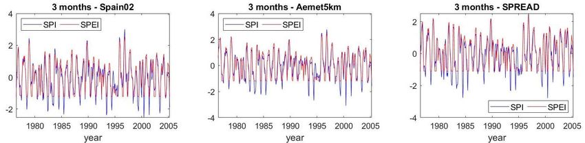
Preprints (www.preprints.org) | NOT PEER-REVIEWED | Posted: 22 March 2022                  doi:10.20944/preprints202203.0291.v1

                                 using various procedures, including physical-based models, regression techniques, artifi-
                                 cial networks and CA models.
                                       Drought analysis is a topic that has generated interest in the research community in
                                 recent years. Numerous studies evaluated the hydrological effect of meteorological
                                 droughts on groundwater [32,33,34,35] or surface flows [36,37,38,39,40]. However, to the
                                 best of our knowledge, there are no studies which have focused on the relationship be-
                                 tween meteorological droughts and hydrological droughts associated with snow dynam-
                                 ics. Neither have we found any studies in the literature that determine the uncertainty of
                                 possible climate change impact on meteorological and SCA droughts using multiple cli-
                                 matic series. Regarding spatial scale, most of the studies have evaluated drought impact
                                 at basin scale [39,41], as well as regions, [42,43,44], countries [45,46,47,48], or entire conti-
                                 nents [49,50], but few [51,52] studies can be found which have focused on alpine systems.
                                       In this article we propose a methodology to assess the impact of potential future sce-
                                 narios (downscaled from RCMs) in meteorological and hydrological droughts in alpine
                                 systems with two novelties. Firstly, the analysis of meteorological and SCA hydrological
                                 droughts where we have used long complete series of SCA obtained with a CA model.
                                 Different uncertainty sources were considered to generate local scenarios: different his-
                                 torical climate databases, simulations (control scenarios and future scenarios), and differ-
                                 ent statistical downscaling techniques. We considered the uncertainty in the historical pe-
                                 riod inherent to different climate products. Secondly, we have studied the correlation be-
                                 tween meteorological droughts and hydrological droughts associated with SCA. We have
                                 used the Sierra Nevada mountain range (southern Spain) as a case study, which is a semi-
                                 arid alpine system very sensitive to the impact of climate change.
                                       We considered different climate information sources (climate products/databases) to
                                 determine the historical drought uncertainty. These climate tools are used to determine
                                 meteorological variables (precipitation and effective precipitation), which are necessary
                                 to compute the proposed meteorological drought indices (SPI and SPEI). We have ana-
                                 lysed the correlation between meteorological drought series and hydrological drought se-
                                 ries (SSCI, associated with SCA) to study their relationship within historical and potential
                                 future scenarios. We have aimed to assess whether information on meteorological
                                 drought can be extracted from SCA dynamics. Future projections of climate variables (pre-
                                 cipitation and temperature) have been obtained by downscaling RCMs to adapt them to
                                 local conditions. We used equi-probable sets of projections, which provide more robust
                                 results than individual models [53,54]. We generated multiple future SCA and climate
                                 series (with a SWG) to assess uncertainty in potential future droughts.
                                       This article is organized as follows: Section 2 describes the case study and available
                                 data and presents the methodology used to assess the potential impact of climate change
                                 and its uncertainty in droughts. Section 3 is dedicated to the analysis of the results. Section
                                 4 discusses the main study aspects. Section 5 presents the main conclusions.

                                 2. Materials and Methods

                                 2.1. Study region
                                       The case study used is the Sierra Nevada mountain range, located in southern Spain
                                 (in the provinces of Granada and Almería) (see Fig.1). It is a linear mountain range, 90 km
                                 long and 20 km wide, parallel to the Mediterranean coast. It is recognized by several pro-
                                 tection agencies (Natural Park, National Park, Biosphere Reserve) and occupies an area of
                                 more than 2,000 km2. It is one of the highest mountain ranges in Europe, with more than
                                 20 peaks with altitudes above 3,000 m.a.s.l.. This mountain range contains the highest
                                 peak in the Iberian Peninsula - Mulhacen - with an altitude of 3,478,6 m.a.s.l.. The Sierra
                                 Nevada enjoys a high mountain Mediterranean climate, with dry summers and wetter
                                 winters, with precipitation that falls almost exclusively in snow form (from November to
                                 May) at altitudes above 2,000 m.a.s.l.. The snow dynamics have a notable effect on the
                                 region from an economic point of view - it is the most southern ski resort in Europe - and
                                 from an environmental and water resources perspective, with a hydrographic network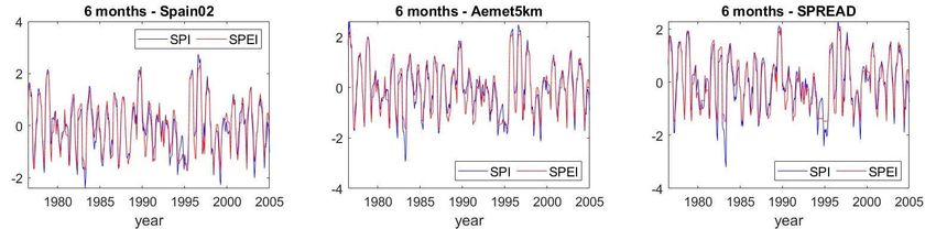
Preprints (www.preprints.org) | NOT PEER-REVIEWED | Posted: 22 March 2022                doi:10.20944/preprints202203.0291.v1

                                 that is mainly fed by snow in the melt season. The weather conditions fluctuate temporar-
                                 ily with high spatial variability due to the topography. Due to these particular conditions,
                                 it is included in the Global Change in Mountain Regions network [55].

                                 Figure 1: Case study location.

                                 2.2. Datasets and Preprocessing

                                 2.2.1. Historical weather data
                                      In this area various meteorological stations networks are available, which generally
                                 have a lack of data at more than 2,000 m.a.s.l.. In this study we used different climate tools
                                 (Spain02 [56,57], Aemet5km [58], SPREAD & STEAD [59,60]) available in Peninsular Spain
                                 (given the insufficient climate data spatial distribution at high elevations), to assess the
                                 impact of climate change on droughts. We used the historical reference period 1976-2005
                                 as the basis for evaluating climate change signal. The climate data sets used do not provide
                                 adequate information on altitudinal gradient due to the low spatial resolution (5 and 12.5
                                 km), so we decided to carry out a drought study referring to the whole of the Sierra Ne-
                                 vada mountain range. We used lumped climate series (using a monthly record weighted
                                 average) to homogenize climate records at mountain range scale. The weights were de-
                                 fined as the area represented by each point with information from climate tools by apply-
                                 ing the Thiessen polygon method [61].

                                 2.2.2. Spain02
                                      We used historical data provided by the Spain02 project [56,57]. It includes daily pre-
                                 cipitation and temperature estimates from observations (around 2,500 quality-control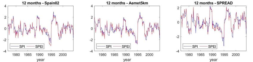
Preprints (www.preprints.org) | NOT PEER-REVIEWED | Posted: 22 March 2022               doi:10.20944/preprints202203.0291.v1

                                 stations) of the Spanish Meteorological Agency. An assessment of the validation of some
                                 Spanish datasets (including Spain02) was recently made by Quintana-Seguí et al [62]. We
                                 used version 5 (v5) of the Spain02 dataset. The project uses the same grid as EURO-
                                 CORDEX project with a spatial resolution of 0.11º (approximately 12.5 km). The Spain
                                 dataset has already been used in many research studies [63,64]. We only selected climate
                                 dataset points included within the Sierra Nevada (or in its vicinity). These points were
                                 distributed topographically at heights between 558 and 2,420 m.a.s.l. (see Fig. 1).

                                 2.2.3. Aemet5km
                                      The Aemet5km project includes daily precipitation and temperature data estimated
                                 from 3,236 precipitation stations observations and 1,800 thermometric stations from the
                                 State Meteorological Agency National Data Bank, with a 5 km spatial resolution. We se-
                                 lected 58 stations from precipitation data set (v.2) and temperature data set (v.1) that var-
                                 ied in heights between 647 and 2,686 m.a.s.l. (see Fig. 1).

                                 2.2.4. SPREAD & STEAD
                                      The SPREAD data set [56] contains estimated daily precipitation data from 11,513
                                 observations coming from the State Meteorological Agency, Agriculture and Environ-
                                 ment Ministry (MAGRAMA) and regional hydrological and meteorological services sta-
                                 tions, with a 5 km spatial resolution. Daily temperature data were obtained from STEAD
                                 dataset [57], which includes estimated temperature data from 5,056 observations from the
                                 State Meteorological Agency and MAGRAMA stations with a 5 km spatial resolution. The
                                 climate points selected varied in height from 300 to 3,230 m.a.s.l. (see Fig. 1).

                                 2.2.5. Climate characterization
                                       Average annual precipitation ranges between 509-657 mm year-1 in the Sierra Ne-
                                 vada, occurring mainly between early autumn and spring (October to April). Precipitation
                                 is mainly associated with North Atlantic and Mediterranean oscillations [65]. Average an-
                                 nual temperature varies between 9.6 and 11.4 ºC, with minimums in January (3 to 5.7 ºC)
                                 and maximums in August (19.3 to 21.8ºC). These temperatures refer to the whole of the
                                 Sierra Nevada National Park, which explains why the minimum temperatures exceed the
                                 0 ºC barrier.
                                       We examined the correlation of the climate variables (as an average study time pe-
                                 riod) with elevation for the different climate tools. We also analysed the altitudinal gradi-
                                 ent of the climate variables with elevation. Linear correlation with elevation is most evi-
                                 dent for temperature, with R2 from 0.87 to 0.97 (see Fig. 2b), which for precipitation, with
                                 R2 more disparate ranging from 0.4 to 0.76 (see Fig. 2a). Precipitation and temperature
                                 show a marked spatial heterogeneity in the study area (with wide altitudinal gradients),
                                 which is common in mountainous regions. Precipitation shows a positive altitudinal gra-
                                 dient (see Fig. 2a), with increases in precipitation with altitude. The opposite is observed
                                 for temperatures, which decrease the higher the elevation is (showing a negative altitudi-
                                 nal gradient) (see Fig. 2b).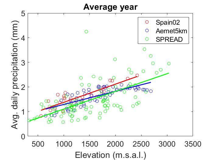
Preprints (www.preprints.org) | NOT PEER-REVIEWED | Posted: 22 March 2022                     doi:10.20944/preprints202203.0291.v1

                               (a)                                                            (b)
                                 Figure 2: a) Daily precipitation average variation with elevation for the different databases. b) Daily
                                 temperature average variation with elevation for the different databases.

                                      Temperature correlations with elevation remain relatively constant throughout the
                                 year, with R2 from 0.8 to 0.98 (see Fig. 3a). Precipitation shows a more irregular temporal
                                 evolution, with R2 from 0.1 to 0.9 (see Figure 3c). The temperature altitudinal gradient
                                 with elevation (TAGE) based on mean temperatures shows a clear difference between cli-
                                 mate databases. The Aemet5km tool shows a pronounced TAGE based on daily means,
                                 with lower gradients in winter (-5.9 º C km-1 in December) and more pronounced in spring
                                 and summer (-7.4 ºC km-1 in March, April, May and June). In contrast, the Spain02 and
                                 STEAD tools show lower TAGE with little variation throughout the year, with gradients
                                 that vary between - 4.9 ºC km-1 in December and - 5.4 ºC km-1 in May and between - 3.8 ºC
                                 km-1 in December and - 4.5 ºC km-1 in April, respectively (see Fig. 3d). Vertical precipita-
                                 tion gradients are the consequence of air rising and stinking as it passes over the mountain
                                 ridge. Its values are positive on the windward side, whilst on the leeward side the values
                                 are negative, increasing when the distance from the mountain increases. In the study area
                                 the precipitation altitudinal gradient with elevation (PAGE) follows the same pattern with
                                 different climate tools, with pronounced variations in winter and almost non-existent in
                                 summer (see Fig. 3b). PAGE based on monthly average precipitation reaches minimum
                                 values in summer, with values that vary between + 1.2 to + 0.058 mm km-1 in August,
                                 increasing significantly for the rest of the year (autumn, winter and spring), with maxi-
                                 mum values varying from + 33.4 to + 48.1 mm km-1 in December (see Fig. 3b).

                                 2.2.2. Snow cover data
                                      SCA data from the historical period (1976-2005) and future period (2071-2100) are
                                 provided from a previous study published by Collados-Lara et al. [61]. In this study we
                                 have used a CA model based on one developed by Pardo- Igúzquiza et al. [66,67] to sim-
                                 ulate SCA using climate indices (precipitation and temperature) as descriptive variables
                                 and a series of parameters (threshold precipitation, threshold temperature and threshold
                                 in the number of neighbour cells that produce a change in the cell state) This model uses
                                 a series of transition rules that allows us to determine the absence or presence of snow. It
                                 has proven to be a useful tool for accurately simulating SCA dynamics [64,66,67].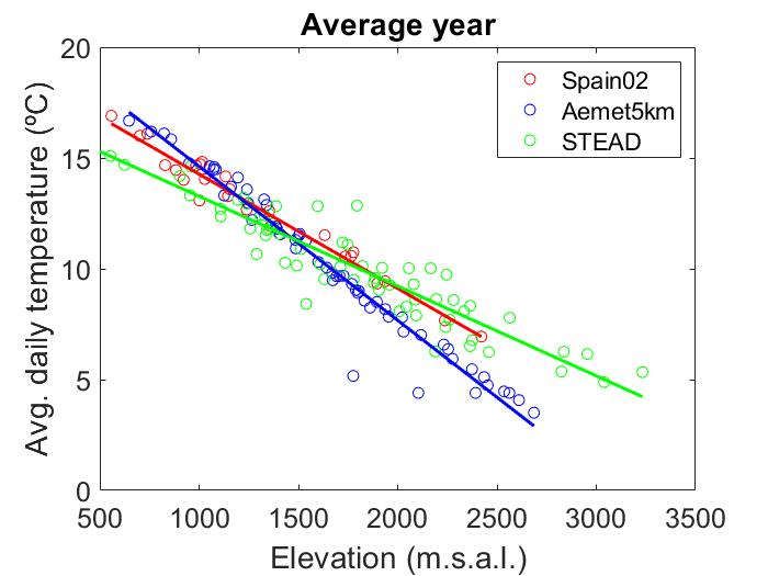
Preprints (www.preprints.org) | NOT PEER-REVIEWED | Posted: 22 March 2022                     doi:10.20944/preprints202203.0291.v1

                                                     (a)                                                 (b)

                                    (c)                                                        (d)

                                 Figure 3: a) Precipitation temporal linear correlation coefficient with elevation for the different da-
                                 tabases. b) Temperature temporal linear correlation coefficient with elevation for the different data-
                                 bases c) Aggregate precipitation temporal altitudinal gradient for the different databases. d) Aggre-
                                 gate temperature temporal altitudinal gradient for the different databases.

                                 2.2.3. Regional climate models
                                       We considered the most pessimistic CORDEX project emission scenario (RCP 8.5)
                                 [68]. For this scenario we analysed nine RCMs nested to four different Global Climate
                                 Models (GCMs) (CNRM-CM5, EC-EARTH, MPI-ESM-LR and IPSL-CM5A-MR). These se-
                                 ries (control scenarios and future simulations of the CORDEX EU project) from five RCMs
                                 (CCLM4-8-17, RCA4, HIRHAM5, RACMO22E and WRF331F) nested in each GCM con-
                                 sidered were used to assess possible future climate scenarios in the period 2071-2100.
                                 RCM simulations considered are summarized in Table 1.

                                 Table 1: Selected Regional Climate Models (RCM) and Global Climate Models (GCM).

                   GCM
             RCM               CNRM-CM5                    EC-EARTH              MPI-ESM-LR                    IPSL-CM5A-MR
          CCLM4-8-17              X                            X                      X
             RCA4                 X                            X                      X
           HIRHAM5                                             X
          RACMO22E                                             X
           WRF331F                                                                                                    X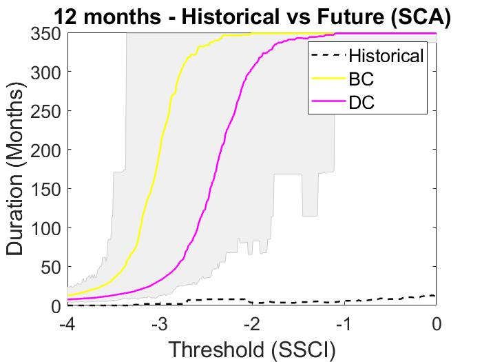
Preprints (www.preprints.org) | NOT PEER-REVIEWED | Posted: 22 March 2022               doi:10.20944/preprints202203.0291.v1

                                 2.3. Methods
                                       We propose a methodology to study historical meteorological and hydrological SCA
                                 droughts and the potential future impact on them in alpine regions for different time ag-
                                 gregation periods (see Fig. 4). Several uncertainty sources are considered. The historical
                                 information used is derived from different climate products. Local potential future sce-
                                 narios (based on the historical information) are defined for a specific time horizon (2071-
                                 2100) and emission scenario (RCP 8.5) by using different RCM simulations, downscaling
                                 techniques, and SWG to generate multiple synthetic series, etc. We analysed the temporal
                                 correlation of SPI/SPEI series (defined to study meteorological droughts) and SSCI series
                                 related with SCA dynamics for the study of hydrological droughts. We aim to draw con-
                                 clusions about meteorological droughts which can be inferred from SCA dynamics series
                                 and vice versa. The proposed methodology (see Fig. 4) includes the following steps. 1)
                                 Historical assessment of meteorological (based on precipitation and effective precipitation
                                 series) and hydrological SCA droughts and uncertainties (due to the climate product)
                                 analysis. 2) Future analysis of meteorological and hydrological SCA droughts: 2.1) Define
                                 future local scenarios by applying different statistical correction techniques under two
                                 conceptual downscaling approaches from RCM simulations included in EURO-CORDEX
                                 project; 2.2) multiple climate and SCA series generation by using a SWG that preserves
                                 the main statistics of local future scenarios; 3) correlation analysis between meteorological
                                 and hydrological SCA droughts for different time lags.
                                       We have used two different indices to analyse meteorological droughts: SPI and
                                 SPEI. The SCA drought was evaluated with SSCI (applying the same methodology as for
                                 SPI using SCA data as input). We applied the run theory [69] to determine the drought
                                 statistics. Note that the future drought index values were calculated using the probability
                                 distributions parameters calibrated for the historical observations to perform an adequate
                                 comparison between the historical and future period in order to identify and assess the
                                 impact of climate change [70].

                                 2.3.1. Drought indices

                                 2.3.1.1. Standardized Precipitation Index
                                       SPI requires monthly precipitation data as input. It does not take into account other
                                 variables also related with drought occurrence, such as temperature, evapotranspiration,
                                 wind speed or atmospheric humidity. This index was developed by McKee et al. [25] for
                                 drought analysis and monitoring. The main advantage of SPI is that it can be calculated
                                 on multiple time scales, being comparable in time and space [71,72]. In our case study, we
                                 calculated SPI for different temporal aggregation time scales (3, 6 and 12 months). We
                                 fitted accumulated precipitation data to a gamma distribution [73] and transformed cu-
                                 mulative probability to a standard normal distribution function, with mean zero and
                                 standard deviation one which provides SPI values. We used the Abramowitz and Stegun
                                 approximation [74] to transform cumulative probability in SPI value:

                                                                                                                       (1)
                       SPI = − t −                                           para 0 < H(x) ≤ 0.5

                                                                                                                       (2)
                        SPI = + t −                                          para 0.5 < H(x) < 1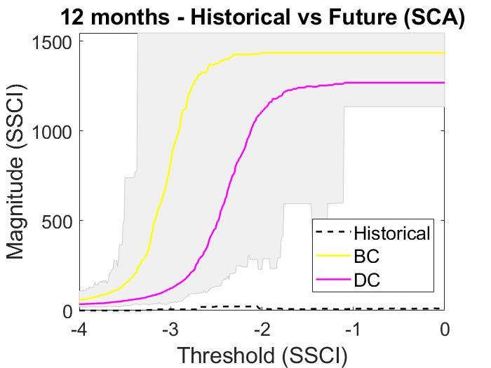
Preprints (www.preprints.org) | NOT PEER-REVIEWED | Posted: 22 March 2022                        doi:10.20944/preprints202203.0291.v1

                                                                                    HYDROLOGICAL DATA

               CLIMATOLOGICAL DATA (P,T)
                                                                      HISTORICAL SCA                      MULTIPLE SERIES OF
          SPAIN02    AEMET5KM      SPREAD&STEAD                          (CA MODEL)                       POTENTIAL FUTURE
                                                                    Collados-Lara et al.(2019)             SCENARIOS (SCA)

                                    HISTORICAL                                                                 (CA MODEL)
               RCM
                                                                                                          Collados-Lara et al.(2019)

                    GENERATION OF POTENTIAL FUTURE SCENARIOS (P, T)

                    BIAS                 FIRST AND SECOND               DELTA
              CORRECTION                MOMENT CORRECTION              CHANGE

                            ENSEMBLE OF FUTURE SCENARIOS (P, T)
                           BIAS CORRECTION            DELTA CHANGE

                           STOCHASTIC WEATHER GENERATOR (P, T)
                                           LARS-WG

               MULTIPLE SERIES OF POTENTIAL                        FIRST AND SECOND
                    FUTURE SCENARIOS (P, T)                      MOMENT CORRECTION

            GENERATION OF METEOROLOGICAL                                            GENERATION OF SNOW COVER
                       DROUGHT INDEX                                                         DROUGHT INDEX

                 SPI (P)            SPEI (P-ETP)                                                  SSCI (SCA)

                    DROUGHT STATISTICS

               FREQUENCY                                            ASSESSNMENT OF THE POTENTIAL
                                        MAGNITUDE
                                                                     IMPACT OF CLIMATE CHANGE ON
                DURATION                INTENSITY                                   DROUGHTS

              LINEAL CORRELATION METEOROLOGICAL AND HYDROLOGICAL DROUGHT INDEX SERIES

         METEOROLOGICAL DROUGHT                     LINEAR REGRESSION MODEL                        SNOW COVER
                     INDEX (X)                      LAGTIME = 0, 1, 2, 3 MONTHS                  DROUGHT INDEX (Y)

     Figure 4: Methodology flowchart.
                                          Where: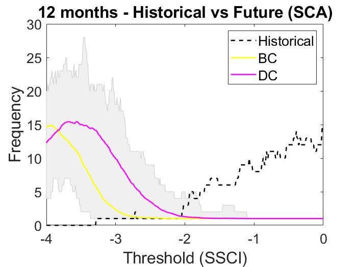
Preprints (www.preprints.org) | NOT PEER-REVIEWED | Posted: 22 March 2022                   doi:10.20944/preprints202203.0291.v1

                                                                                                                            (3)
                        t=    ln                                                para 0 < H(x) ≤ 0.5
                                   ( ( ))

                                                                                                                            (4)
                         t=    ln           ( ))
                                                                               para 0.5 < H(x) < 1
                                     (

                                         where H(x) is cumulative probability and the constants are: c0 = 2.515517, c1 =
                                    0.802853, c2 = 0.010328, d1 = 1.432788, d2 = 0.189269, d3 = 0.001308. Positive SPI values indi-
                                    cate wet periods, with deviations above mean. Negative SPI values reproduce dry peri-
                                    ods, with deviations below mean.

                                   2.3.1.2. Standardized Evapotranspiration Precipitation Index
                                          SPEI developed by Vicente-Serrano et al. [75] (considered an improved SPI) is par-
                                   ticularly useful for analysing climate change effects in drought conditions. SPEI considers
                                   the influence of temperature on drought, preserving SPI multi-scale nature. This index is
                                   based on a climate water balance determined by the difference between precipitation and
                                   potential evapotranspiration in each month i:

                                                        D = P − PET                                                         (5)

                                    where D is effective precipitation, P is precipitation and PET is evapotranspiration. Evap-
                                    otranspiration is calculated by applying the Thornthwaite approximation [76], which only
                                    requires the monthly mean temperature values as input.
                                          The SPEI is calculated following the procedure described in Vicente-Serrano et al.
                                    [75], where cumulative D series fit a 3-parameter Log-Logistic distribution. Di values cal-
                                    culated are added for different time scales (3, 6 and 12 months). To transform the cumu-
                                    lative probability values to the SPEI values, a standard normal distribution, with mean
                                    zero and standard deviation one, is used following the Abramowitz and Stegun approxi-
                                    mation [74]:

                                                              c +c W+c W                                                    (6)
                                               SPEI = W −
                                                            1+d W+d W +d W

                                    where W = −2 ln(p) to p ≤ 0.5 where p is the probability of exceeding a certain value
                                    D, p = 1 − F(x), being F(x) the cumulative probability. If p > 0.5, p is replaced by 1 − p
                                    and the SPEI resulting sign is reversed. The constants are: c0 = 2.515517, c1 = 0.802853, c2 =
                                    0.010328, d1 = 1.432788, d2 = 0.189269, d3 = 0.001308.

                                    2.3.2. Drought statistics
                                          Drought statistics (frequency, duration, magnitude and intensity) were calculated by
                                    applying the run theory [69]. We considered meteorological (SPI and SPEI) and hydrolog-
                                    ical (SSCI) drought index threshold values (ranged from -4 to 0) to identify drought peri-
                                    ods. The frequency is defined as the drought events number that occurs during a certain
                                    time period. Duration is defined as an uninterrupted time period (in months) with index
                                    values below the threshold value. Magnitude is the sum of all the index values during the
                                    duration of the drought. Intensity is the minimum index value in a specific drought event.
                                    Drought statistics values determined for each drought event were averaged for the total
Preprints (www.preprints.org) | NOT PEER-REVIEWED | Posted: 22 March 2022 doi:10.20944/preprints202203.0291.v1
drought events number identified for each threshold.
(7)
M= ÍNDICE
I = Min(ÍNDICE ) (8)
where D is duration, M is mean magnitude and I is the mean intensity of the
drought.
2.3.3. Future drought strategy
We proposed a RCM correction to generate local future scenarios that would pro-
vide reliable estimates of the climate characteristics (precipitation and temperature). The
obtained future climate scenarios are introduced into a SWG to generate multiple cli-
mate series to approach future scenarios uncertainty. We used this multiple climate se-
ries to generate relative drought indices (rSPI, rSPEI and rSSCI), which were calculated
using the probability distributions parameters of the historical series, which allows us to
make an adequate comparison to assess the potential impact of climate change. The gen-
eration of multiple drought index series (using a SWG) allows us to assess climate
change uncertainty in droughts. The multiple local future climate scenarios generation
procedure is described in Sections 2.3.3.1 and 2.3.3.2., and the multiple local future SCA
scenarios were obtained from a previous study [77]
2.3.3.1. Local future scenarios
We used a tool developed by Collados-Lara et al. [78,79] for the generation of future
climate scenarios considering two different downscaling approaches: bias correction (BC)
and delta change (DC). The BC approach applies a transformation function to the control
RCM simulation to obtain another with similar statistics to the historical one. The trans-
formation function is applied to the future simulation to obtain a corrected future sce-
nario. It is assumed that bias between the historical series statistics and the control simu-
lation will remain invariant in the future. The DC approach assumes that RCMs provide
an accurate assessment of the relative changes between the control simulation and the
future simulation and applies these changes to the historical series to obtain a corrected
future series. The transformation function applied in both approaches is defined with the
first and second moment statistical correction technique. Individual future scenarios gen-
erated with the different RCMs were merged making equi-probable ensembles of future
projections with BC and DC approaches, which provide more representative future sce-
narios.
2.3.3.2. Generation of multiple climate series using a stochastic model
SWG allow us to generate synthetic time series with statistical characteristics similar
to future projections scenarios. These generated multiple future scenarios are consistent
with future scenarios predicted with RCMs. The future scenarios generated with BC and
DC approaches are used as input in LARS-WG-SWG [80] to generate multiple future se-
ries. LARS-WG has been updated several times (most recently in April 2021) and can be
used to generate synthetic weather series at a location. It can also be used to generate
potential local future scenarios based on Global Climate Models (GCM) outputs. In this
study we have used LARS-WG to produce multiple synthetic climate time series based on
sets of future local climate scenarios generated with BC and DC approaches (derived from
different local RCM projections). Multiple series generated with SWG may show bias withPreprints (www.preprints.org) | NOT PEER-REVIEWED | Posted: 22 March 2022 doi:10.20944/preprints202203.0291.v1
original series statistics. We corrected these biases using a statistical technique developed
by Collados-Lara et al. [76] based on mean and standard deviation correction.
2.3.3.3. Analysis of the temporal correlation between meteorological drought and snow
cover dynamics
We evaluated the correlation degree between meteorological drought and SCA
drought by applying a linear regression model. Meteorological drought series are as-
sumed as independent variable (x) and SCA drought series as dependent variable (y).
Thus, if consider xi and yi with i = 1, 2, ..., N; linear relationship between variables is de-
termined with determination coefficient:
∑ ( ) (9)
R = 1− with lag time = 0, +1, +2, +3 months.
∑ ( )
where y = β x + β is the fitted linear regression line, being β1 and β0 slope and inter-
cept, respectively, with R2 in the range (0 ≤ R2 ≤ 1). Determination coefficient specifies the
proportion of the independent variable (y) variance that can be linearly attributed to de-
pendent variable (x) variance [81].
3. Results
3.1. Assessment of the meteorological (P & T) and hydrological (SCA) droughts
3.1.1. Historical analysis
Figure 5 shows SPI and SPEI evolution for 3, 6 and 12 months temporal aggregation
scales during the historical period 1976-2005 in the study area. Shorter temporal aggrega-
tion scales (e.g., 3 months) showed more frequent dry and wet period fluctuations. For
higher temporal aggregation scales (e.g., 12 months) dry and humid periods showed
longer but less frequent fluctuations over time. The indices exhibited a similar trend with-
out any notable differences, though it is worth mentioning more accentuated drought pe-
riod detection with SPI, especially for smaller temporal aggregation scales (3 months).
With higher temporal aggregation scales (12 months) influence of evapotranspiration on
droughts becomes more relevant.
SPI and SPEI series showed a similar temporal evolution, which indicates the high
correlation degree between both indices. In order to compare the meteorological drought
indices used we analysed the correlation between SPI and SPEI. Figure 6 shows the deter-
mination coefficient between both meteorological drought indices (SPI and SPEI) for the
different temporal aggregation scales (3, 6 and 12 months). The linear correlation coeffi-
cient calculated between SPI and SPEI ranged from 0.82 to 0.91. The lowest correlations
were detected with the lowest temporal aggregation scales (3 months) for all the climate
databases. These correlations increased for higher temporal aggregation scale, obtaining
the best results for the highest temporal aggregation scale (12 months). Note that SPEI and
SPI have different minimum values (see the horizontal patterns of the data points in Fig-
ure 6. a, b, c, e and f). However the maximum values are similar.Preprints (www.preprints.org) | NOT PEER-REVIEWED | Posted: 22 March 2022 doi:10.20944/preprints202203.0291.v1
(a) (b) (c)
(d) (e) (f)
(g) (h) (i)
Figure 5: SPI and SPEI temporal evolution for the different temporal aggregation scales and data-
bases.
A comparative analysis of meteorological droughts characteristics identifies similar re-
sults between climate databases (see Figs. 8,9,10), but shows significant differences be-
tween SPI and SPEI. SPI-3 shows more extreme events and severe droughts (20) than SPEI-
3 (0), since the latter only identifies moderate and slight droughts (see Figs. 8b, 9b, 10b).
The mean duration of the drought events detected with SPEI-3 was the longest (5 months)
compared with SPI-3, which detects more intense and short droughts periods (2 months).
The mean magnitude of SPI-3 and SPEI-3 shows a similar difference (-3.6 versus -4.2).
Higher SPEI orders show a downward trend with drought events that tend to be more
severe. SPEI-12 detects events with a similar severity that the identified with SPI-12 (- 1.9
vs. - 2 on average) (see Appendix B –Fig. B1h and i, Fig. B2h and i, and Fig. B3h and i). The
difference in the mean duration of drought events detected with SPEI-12 versus SPI-12 is
notable (12 versus 9 months), however, for severe and extreme drought events they aver-
age a similar duration (4 months). SPI-12 detects a higher number of events than SPEI-12
(21 vs.15), but identifies the same frequency of severe drought events (5). In magnitude
terms, the differences between SPI-12 and SPEI-12 are notable (-6.5 vs.-10). Magnitude isPreprints (www.preprints.org) | NOT PEER-REVIEWED | Posted: 22 March 2022 doi:10.20944/preprints202203.0291.v1
a drought severity indicator, so that SPEI provides more severe droughts than SPI (see
Appendix B – Fig. B1f and g, Fig. B2f and g and Fig. B3f and g).
(a) (b) (c)
(d) (e) (f)
(g) (h) (i)
Figure 6: Correlation coefficients between SPI and SPEI indices derived from Spain02 (left column),
Aemet5km (intermediate column) and SPREAD&STEAD (right column) databases for the different
time scales.
Likewise, we analysed hydrological drought (SCA) characteristics in the Sierra Ne-
vada mountain range. A statistical analysis shows significant differences in drought fre-
quency, duration and magnitude for the different temporal aggregation scales, but no
changes were detected in intensity. Lower SSCI values showed greater fluctuations than
higher SSCI values, which show a lesser trend with prolonged dry periods. The number
of drought events identified with SSCI-3 was higher (25) than that detected with SSCI-12
(15). However, SSCI-12 showed longer drought events (11 months) compared to thosePreprints (www.preprints.org) | NOT PEER-REVIEWED | Posted: 22 March 2022 doi:10.20944/preprints202203.0291.v1
obtained with SSCI-3 (5 months). In the same way, magnitude exhibited by SSCI-12 (-9)
far exceeded that identified with SSCI-3 (-4,6) (see Fig. 11 and Appendix B - Fig. B4).
4.1.2. Future analysis
Climate projections under RCP 8.5 emission scenarios based on different correction
approaches (BC and DC) predict a significant reduction in precipitation (27 - 22% on av-
erage) for the 2071-2100 time horizon, with average precipitation varying between 373 to
468 mm year-1 and 381 to 488 mm year-1 for BC and DC approaches, respectively. The
future mean precipitation differs depending on the climate database used. The Spain02
climate tool provides the highest mean precipitation values (468 to 488 mm year-1) (see
Fig. 7a) and the SPREAD database averages the lowest values (373 to 381 mm year-1) (see
Fig. 7e). The Aemet5km climate tool is in an intermediate range, it provides future precip-
itation values that vary on average from 427 to 434 mm year-1 for the BC and DC ap-
proaches, respectively (see Fig. 7c). Regarding temperature a considerable increase is pre-
dicted, which on average stands at 4.5 ºC (for the BC and DC approaches) in relation to
the historical period for all climate tools (see Fig. 7b, d, and f). Note that the BC and DC
generated temperature series have the same mean monthly values, but the series are dif-
ferent. Therefore, both approaches predict the same changes in mean temperatures when
the same historical information is used. However, with each climate database the predic-
tions showed different mean temperatures for the mean year in the future. Note that the
historical series of the different databases are different. The mean temperatures predicted
vary from 14.3 to 16.1 °C for the BC and DC approaches respectively. The STEAD database
predicted the highest mean temperatures (16.1 °C), whilst the Aemet5km climate tool pre-
dicted the lowest means values (14.3 ºC). The predictions made with the Spain02 database
are in an intermediate range, with 15.9 ºC mean temperature values. In alpine systems,
another relevant aspect related to climate conditions is SCA. Maximum SCA annual peri-
ods in the 1976-2005 historical period are reached in winter months (January and Febru-
ary), with 449 and 439 km2 covered by snow, respectively. On the contrary, in summer
(July and August) the SCA is practically nil (see Fig. 7g). Future projections of SCA for the
BC and DC approaches predict a significant reduction in annual SCA for the 2071-2100
future period, with a reduction of snow season of 2 months (May to October) with 195 and
176 km2 and 227 and 209 km2 maximum values in January and February for the BC and
DC approaches, respectively (see Fig. 7g). This represents an average annual SCA reduc-
tion from 79% and 75% for the BC and DC approaches, respectively, whilst in peak months
(January and February) a reduction of 57% and 49% in January and 59% and 52% in Feb-
ruary is predicted for the BC and DC approaches.
Variations in climate conditions and SCA dynamics have a determining effect on fu-
ture meteorological and hydrological droughts. Under an RCP 8.5 emission scenario, me-
teorological drought showed a significantly increasing trend in the study area with all the
climate tools. SPI-3 suffered an increase in mean number of severe drought events for the
Spain02 (27 vs. 21) and Aemet5km (22 vs. 18) climate databases compared to observed
period (see Figs. 8.a and 9.a). Severe drought duration showed a similar contrast with the
historical one for SPI-3, but we observed a generalized increase in duration for Spain02 (7
versus 4 months) (see Fig. 8c), Aemet5km (6 vs. 4 months) (see Fig. 9c) and SPREAD (6 vs.
4 months) climate products (see Fig. 10c). Likewise, we identified an increase in drought
severity in relation to the observed period for Spain02 (-6.5 vs.-3.6) (see Fig. 8e), Aemet5km
(-5.5 vs. -3.6) (see Fig. 9e) and SPREAD (-5.5 vs. - 3.7) climate products (see Fig. 10e). In
contrast, no significant variation in drought intensity is detected in the future in any da-
tabase. Statistical studies with SPEI-3 do not reveal significant changes in the number of
drought events detected in the future, except the analysis with SPREAD&STEAD climate
tool, which shows a lower number of drought episodes compared to the reference period
(34 vs. 43) (see Fig. 10b). However, the duration of droughtPreprints (www.preprints.org) | NOT PEER-REVIEWED | Posted: 22 March 2022 doi:10.20944/preprints202203.0291.v1
(a) (b)
(c) (d)
(f) (g)
(h)
Figure 7: a) Historical and future average precipitation with uncertainty range (Spain02); b) Histor-
ical and future average temperature with uncertainty range (Spain02); c) Historical and future av-
erage precipitation with uncertainty range (Aemet5km); d) Historical and future average tempera-
ture with uncertainty range (Aemet5km); e) Historical and future average precipitation with uncer-
tainty range (SPREAD); f) Historical and future average temperature with uncertainty range
(STEAD); g) Historical and future average SCA with uncertainty range.Preprints (www.preprints.org) | NOT PEER-REVIEWED | Posted: 22 March 2022 doi:10.20944/preprints202203.0291.v1
events identified with SPEI-3 was much higher than that observed in the historical period
with Spain02 (9 vs. 5 months) (see Fig. 8d), Aemet5km (9 vs. 5 months) (see Fig. 9d) and
SPREAD&STEAD (9 vs. 5 months) (see Fig. 10d) climate databases. In the same way, the
magnitude of the droughts is accentuated with all the climate tools. However, there are
no significant changes in drought intensity in all climate products (see Fig. 10e).
In the long term, both SPI and SPEI show a considerable increase in the number of
extreme and severe droughts detected in relation to the observed period. We also pre-
dicted an increase in drought duration. For example, the results obtained on average with
respect to the observed period with Spain02 (82 vs. 8 months for SPI-12 and 131 vs.10
months for SPEI-12), Aemet5km (74 8 months for SPI-12 and 196 vs. 10 months for SPEI-
12) and SPREAD&STEAD (74 vs. 10 months for SPI-12 and 196 vs. 17 months for SPEI-12)
climate products, with drought events that were longer for scenarios generated with the
BC approaches. Future drought severity (2071-2100), shows mean magnitudes that far ex-
ceeded the values identified in the reference period (1976-2005) for Spain02 (-100.2 vs. -5.9
for SPI-12 and -206.9 vs. -7.8 for SPEI-12), Aemet5km (-74.1 vs. -6 for SPI-12 and -272.6 vs.
-8 for SPEI-12) and SPREAD&STEAD (-74.1 vs. -7.6 for SPI-12 and -272.7 vs. -14.2 for SPEI-
12) databases. Likewise, we revealed more intense droughts for the RCP 8.5 emission sce-
nario with SPI-12 and SPEI-12 in all climate databases (see Appendix B –Figs. B1, B2 and
B3).
Hydrological drought statistics for the 3 month temporal aggregation scale can be
seen in Figure 11. Hydrological droughts at lower temporal aggregation scales (3 months)
showed less extreme and severe drought events, with SSCI values that never exceed the -
1.5 barrier in the future. Predictions revealed that there was no variation in the number of
drought events compared to the reference period, but there was a notable increase in the
duration of these events (8 months for the BC approach and 7 months for the DC ap-
proach, vs. 5 months). Drought magnitude showed similar differences (-5.6 and -5.7 for
the BC and DC approaches, respectively, vs. -4.6), which is due to the remarkable reduc-
tion that was observed in the mean drought intensity (-1.2 for BC and DC approaches vs.
-1.8). These results contrast with those obtained for the higher temporal aggregation scale,
with droughts that were much more intense in the future (-6.2 for BC approach and -5.8
for the DC approach vs. -2.1). Future predictions for hydrological SCA droughts showed
a continuous extreme drought time period in the Sierra Nevada with the BC approach,
with a single drought event for the entire analysed period (349 months). Similar results
were revealed with the DC approach, with a single extreme drought event that lasted most
of the study time period (303 months). Drought magnitude is much higher (-1436.6 for the
BC approach and -1269.6 for DC approach, vs. -8.9) compared to the reference period (See
Appendix B –Fig.B4).
4.1.2. Assessment of the correlations between meteorological (P & T) and hydrological
(SCA) droughts
We analysed the linear correlation between multiple meteorological (SPI and SPI)
drought indices and the hydrological (SSCI) drought index series (generated with BC and
DC correction approaches). Mean values of these correlations for the BC and DC ap-
proaches are shown in Figure 12. The SCA dynamics response to meteorological condi-
tions was identified with a 0 to 3 months time lag (see Fig. 12). In general, the SCA re-
sponse to weather conditions depends on the climate characteristics (temperature and rel-
ative humidity). The highest correlation values occurred for smaller temporal aggregation
scales (3 and 6 months) with short response times (0 to 1 months). In general, correlations
decreased significantly on the longest time aggregation scale (12 months). It should be
noted that correlation was slightly higher with SPEI. In particular, from the climate data-
bases used, it should be noted that the meteorological drought series produced with
Spain02 had a higher correlation with the hydrological drought series (SSCI). For drought
propagation, the 1 month response time seems to be a turning point in all thePreprints (www.preprints.org) | NOT PEER-REVIEWED | Posted: 22 March 2022 doi:10.20944/preprints202203.0291.v1
(a) (b)
(c) (d)
(f) (g)
(h) (i)
Figure 11: Historical and future meteorological drought statistics (frequency, duration, magnitude
and intensity) derived from SPI (left column) and SPEI (right column) deduced with Spain02 data-
base.Preprints (www.preprints.org) | NOT PEER-REVIEWED | Posted: 22 March 2022 doi:10.20944/preprints202203.0291.v1
(a) (b)
(c) (d)
(e) (f)
(g) (h)
Figure 9: Historical and future meteorological drought statistics (frequency, duration, magnitude
and intensity) derived from SPI (left column) and SPEI (right column) deduced with Aemet5km
database.Preprints (www.preprints.org) | NOT PEER-REVIEWED | Posted: 22 March 2022 doi:10.20944/preprints202203.0291.v1
(a) (b)
(c) (d)
(e) (f)
(g) (h)
Figure 10: Historical and future meteorological drought statistics (frequency, duration, magnitude
and intensity) derived from SPI (left column) and SPEI (right column) deduced with
SPREAD&STEAD database.Preprints (www.preprints.org) | NOT PEER-REVIEWED | Posted: 22 March 2022 doi:10.20944/preprints202203.0291.v1
(a) (b)
(c) (d)
Figure 11: Historical and future hydrological SCA drought statistics (frequency, duration, magni-
tude and intensity) derived from SSCI.
temporal aggregation scales. The highest correlation in the reference period 1976-2005
(0.63) occurred in the 3 month temporal aggregation scale with an immediate response
time (0 months). Thus, this indicates that the corresponding month climate condition
was the most significant variable that contributed to the SCA dynamics in the Sierra Ne-
vada.
In general, the SPI mean correlations with SSCI are higher in the future, especially in
the lower temporal aggregation scales. In contrast, the SPEI shows slightly lower correla-
tions with the SSCI. However, the maximum mean correlation took place with the SPEI in
3 month temporal aggregation scale with no delay in hydrological drought response, with
a 0.69 value for the Spain02 climate tool. In contrast, the highest SPI mean correlation
(0.66) occurred with a 1 month time lag.
5. Discussion
Climate models provide essential information to study the impact of climate change on
droughts. However, there is high uncertainty in scenarios generated from GCM and RCM
simulations that may cause a drought persistence underestimation [82], therefore an un-
certainties analysis associated with climate models must be incorporated. One way to re-
duce this uncertainty in the climate projections is to merge multiple RCMs, which provide
more robust results than individual models [83]. SWGs are useful tools to take into ac-
count uncertainty by generating equi-probable multiple weather series preserving the val-
ues identified in some statistics for the future climate. SWG has been used extensively in
previous studies to assess the impact of climate change [84,85]. In this study we have usedPreprints (www.preprints.org) | NOT PEER-REVIEWED | Posted: 22 March 2022 doi:10.20944/preprints202203.0291.v1
a SWG to quantify the climate change uncertainty in meteorological and hydrological
droughts associated with SCA.
(a) (b)
(c) (d)
(e) (f)
Figure 12: Correlations between meteorological and hydrological SCA droughts for different re-
sponse times with SPI (left column) and SPEI (right column) in the different temporal aggregation
scales.Preprints (www.preprints.org) | NOT PEER-REVIEWED | Posted: 22 March 2022 doi:10.20944/preprints202203.0291.v1
Most studies have used standardized indices with multi-scale properties, compara-
ble in time and space, for drought analysis and monitoring [86,87,88]. In our study we
have used SPI and SPEI indices for meteorological droughts and a novel variant of the SPI
(SSCI) for hydrological droughts to assess the impact of climate change (and its uncer-
tainty) on multiple time scales. These indices require continuous climate records (precip-
itation and temperature) over a long enough time period. Climate tools contain continu-
ous climate records (precipitation and temperature) over a long period of time with a fixed
spatial scale and are useful in areas where data are scarce (such as alpine areas). In this
study we used the climate products available in Peninsular Spain (Spain02, Aemet5km
and SPREAD & STEAD). Other researchers have analysed the impact of climate change
(and its uncertainty) on droughts in other regions [89,90], but not in the Sierra Nevada
mountain range. Nevertheless, the methodology applied in this study is a parsimonious
approach applicable to any case study. Only historical SCA and climate data and future
RCM and SCA climate data are needed to assess the impact of climate change (and its
uncertainty) on meteorological and hydrological droughts.
Drought characteristics (including frequency, duration, magnitude and intensity)
have an implicit or explicit relationship with the established temporal aggregation scale.
In general, long temporal aggregation scale indices are more likely to indicate moderate
droughts that persist for long periods of time, whilst short temporal aggregation scales
indicate more severe droughts with short durations [91]. In this article, behaviour analysis
of each temporal aggregation scale in meteorological and hydrological drought detection
in reference period agrees with the above observation. Results in the reference period
(1976-2005) revealed high correlations between SPI and SPEI in each temporal aggregation
scale, which indicates that precipitation variability is the main meteorological drought
driver. For the 1976-2005 historical period the meteorological droughts studied with SPEI
identified more serious droughts that manifested for a longer time compared to those de-
tected with SPI in each temporal aggregation scale, which shows the importance of con-
sidering potential evapotranspiration in drought analysis. However, despite what we
might expect, the most intense droughts were detected with SPI. Although most research
refers to the greater capacity of SPEI to identify droughts [92,93,94] there is no common
agreement regarding the severity detected. In some studies in semi-arid regions higher
intensities were detected with SPI [94,95,96], whilst in others a higher severity was always
identified with SPEI [97]. Other investigations showed more extreme droughts with SPI
at lower temporal aggregation scales, although similar or even slightly higher intensities
were identified in higher accumulation periods with SPEI [98]. In this study although the
droughts were generally more extreme with SPI, we only identified slightly more severe
droughts with SPEI at longer temporal aggregation scales. These results are consistent
with other investigations in the Mediterranean region [99,100], where precipitation varia-
bility controls drought occurrence.
For the 2071-2100 horizon under RCP 8.5 emission scenario climate change impact
on meteorological droughts in the Sierra Nevada is very significant. Future scenarios in-
dicate a reduction in precipitation from 22 to 27% and an increase in 4.5ºC average tem-
perature at the end of the 21st century, which is consistent with other studies that evalu-
ated climate change impact in Mediterranean region [101,102,103]. This notable alteration
in future climate conditions explains the significant impact on droughts. Despite relevant
uncertainty, we expected a general increase in drought severity and duration. Future
drought scenarios based on SPI showed less significant changes compared to SPEI. When
considering temperature effect, SPEI-based scenarios show a clear trend towards drasti-
cally more severe and prolonged droughts. However, both SPI and SPEI detected consid-
erable deviations from normal conditions in the reference period. Several studies that
used SPI and SPEI indices to assess the impact of climate change on meteorological
drought in semi-arid regions reached the same conclusions [104,105]. These results
demonstrate that temperature is the dominant factor contributing to increased drought
compared to other factors such as precipitation. The importance of considering potentialPreprints (www.preprints.org) | NOT PEER-REVIEWED | Posted: 22 March 2022 doi:10.20944/preprints202203.0291.v1
evapotranspiration in drought analysis under global warming scenarios has been high-
lighted in previous studies [75], thus demonstrating the consistency of our results.
SCA analysis in RCP 8.5 (the higher emission scenario) revealed a very considerable
impact on hydrological droughts. During winter (December to March) we expected re-
ductions from 46 to 66% in SCA, although further reductions are expected in the rest of
the year. This significant impact on SCA has a direct effect on hydrological droughts, with
a general increase in drought magnitude, severity and duration. Other studies have also
demonstrated the significant impact of climate change on SCA in other mountain ranges
[106,107,108], however, there are no studies that have evaluated impact of climate change
on SCA droughts.
We have also analysed the correlation of SSCI with the SPI and SPEI using a linear
regression model for the different accumulation periods to identify temporal aggregation
scale in which precipitation and effective precipitation deficits propagate through hydro-
logical cycles to produce deficits in SCA. Another possible option would be to use the
cross-wavelet analysis, which is a robust method that shows how the components of the
time series are coherent in the time-frequency domain and provides phase lag infor-
mation. The cross-wavelet analysis has been used in other research to study the coherency
between the seasonal components of climate and vegetation time series and provide the
phase lag [106,107], and investigate the relationship between the climate indices and
drought/flood conditions [108,109], amongst others. In this study the precipitation SCA
relationship reflects an important correlation coefficient between meteorological and hy-
drological droughts. The SSCI series revealed a good correlation with SPI and SPEI series
in lower temporal aggregation scales (3 and 6 months), but we observed a considerable
reduction in the relationship for the 12-month temporal aggregation scale. The SPEI series
showed a higher correlation with SSCI series, which shows the effect of temperature on
SCA dynamics. Other researchers have identified the influence of climate variables on the
snow dynamics in the Sierra Nevada [13,14]. These studies identified the precipitation
regime as the main snow dynamics driver, not underestimating the influence of tempera-
ture. Correlations between meteorological and hydrological droughts show good correla-
tions for short response times in the different SPI and SPEI accumulation periods. Alt-
hough the strongest correlation occurs when SPEI is not lagged, the presence of weak cor-
relations in time lags of several months demonstrates the lack of early warning potential
for hydrological droughts based on the persistence of meteorological anomalies.
6. Conclusions
We proposed a methodology to evaluate the potential impact of climate change (and
its uncertainty) for meteorological and hydrological droughts. We have generated local
ensemble scenarios from RCMs by combining the results obtained with different statisti-
cal downscaling techniques under the BC and DC approaches. We applied a SWG to gen-
erate multiple series based on the generated ensemble local scenarios. Relative standard-
ized indices have been used to assess the impact of climate change on meteorological (SPI
and SPEI) and hydrological (SSCI) droughts at different time scales. We have analysed
drought frequency, duration, magnitude, and intensity trends to better understand tem-
poral changes in drought characteristics.
The methodology is applicable to any case study. We have applied it to the Sierra
Nevada mountain range, which is an alpine area highly sensitive to climate change. For
the most pessimistic emission scenario, RCP 8.5, we estimated a reduction from 27 to 22%
in precipitation and an increase of 4.5 ºC in temperature at the end of the 21st century,
which will affect SCA dynamics with a reduction of 2 months for the snow season and an
average reduction from 79 to 75% in the annual SCA. Meteorological drought analysis
revealed the usefulness of SPEI evaluating drought characteristics in climate change sce-
narios, due to the fundamental role of temperature in potential evapotranspiration. De-
spite relevant uncertainty, our results showed that climate change scenarios lead to a gen-
eralized increase in both meteorological and hydrological drought statistics, with aYou can also read