Analisi di Immagini e Video (Computer Vision) - Giuseppe Manco
←
→
Page content transcription
If your browser does not render page correctly, please read the page content below
Analisi di Immagini e Video
 (Computer Vision)
 Giuseppe Manco
Outline
• Segmentation
• Approcci classici
• Deep Learning for Segmentation
Crediti
• Slides adattate da vari corsi e libri
 • Computational Visual Recognition (V. Ordonez), CS Virgina Edu
 • Computer Vision (S. Lazebnik), CS Illinois Edu

Approcci supervisionati
• L’approccio basato su CRF è semi-supervisionato
• Possiamo renderlo supervisionato?
 • Parametrizziamo gli unary e binary potentials
 "
 • E.g., ! ! ; = exp $ ⋅ !
 # !
 • Apprendiamo i parametri che minimizzano l’energia media su tutti gli esempi
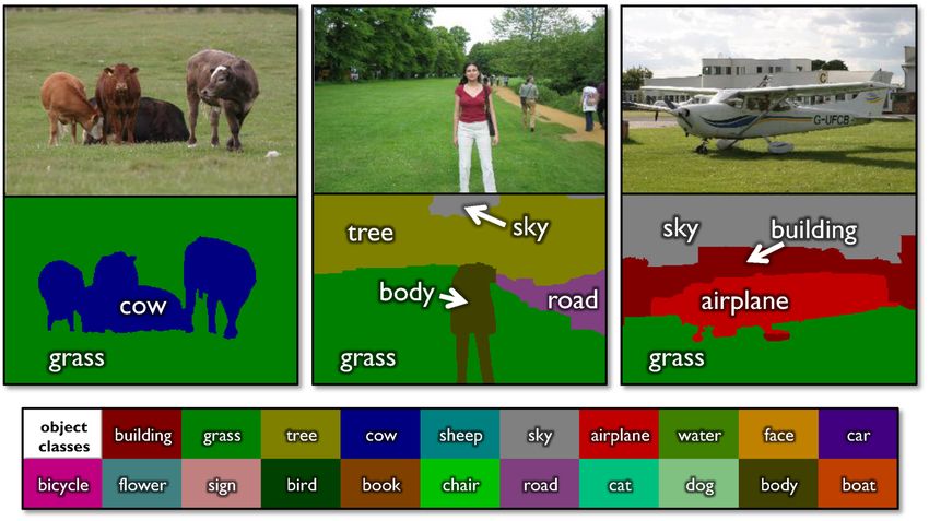
Semantic segmentation, object detection
• Problema
 • Etichettare ogni pixel con una classe
 • Multi-class problem
• Utilizzo di dati già etichettati
 • Pascal VOC
 • MS COCO
MS-COCO

• Large-scale dataset for object detection, segmentation and captioning
 • 330K images (>200K labeled)
 • 1.5 million object instances
 • 80 object categories
 • 91 stuff categories
 • 5 captions per image
 • 250,000 people with keypoints
Perché Deep Learning?
• Stesso principio dell’object detection
 • Convolutional features, learned from training data
• Accuratezza
• Velocità
Approcci
• Approcci downsampling-upsampling
• Metodi multi-scala
Fully Convolutional Networks
• Utilizziamo i layer convoluzionali per fare le predizioni sui vari pixel
Fully Convolutional Networks
• Utilizziamo i layer convoluzionali per fare le predizioni sui vari pixel
 • Ma fare convoluzioni su feature map grandi è costoso
Fully Convolutional Networks
• Soluzione
 • Architettura Encoder-Decoder

 upsampling

 Input Output

 downsampling
Convolutionalization
• Fully Convolutional Layers
• Faster-RCNN, SSD
Fully Convolutional Networks
• Architettura Encoder-Decoder

 upsampling

 Input Output

 downsampling
 Convolution, Pooling
Fully Convolutional Networks
• Architettura Encoder-Decoder

 upsampling Unpooling,
 Transposed
 convolution

 Input Output

 downsampling
Up-sampling Convolutions

• Upsampling
 • Da un’input a bassa risoluzione si
 passa ad uno a più alta
 risoluzione
 • Transposed Convolution
 • Qual è la relazione?
 • Suggerimento: invertiamo le
 relazioni originarie

 https://github.com/vdumoulin/conv_arithmetic
Transposed Convolution
Transposed Convolution
Transposed Convolution
Transposed Convolution
• Ogni valore si distribuisce su un intorno dell’output in base al kernel.

• La distribuzione viene guidata da padding e stride
Convolution e transposed convolution
• Ogni riga definisce
 un’operazione di
 convoluzione
 • Filtro 3x3, input 4x4
 • No padding, no strides, no
 dilation
Convolution e transposed convolution
• Ogni riga definisce un’operazione di convoluzione
Convolution e transposed convolution
• Trasponendo la matrice di convoluzione, otteniamo l’operazione
 opposta
ConvTranspose, Padding
• Decrementa l’output della TD
 • Interpretazione: l’ammontare di padding che l’input richiede per completare
 l’output
 • Quale sarebbe l’output dell’esempio precedente?
ConvTranspose, Stride
• Espande l’output
 • Di conseguenza «fraziona» l’input aggiungendo spazi
 Il filtro si muove di 2
 pixel sull’output
ConvTranspose, checkerboarding
 • Filter [ - , . , / ], output stride = 2

 ! " # $ % & ' (
 input
 stride 2

 output

 ! !

 Animation: https://distill.pub/2016/deconv-checkerboard/
ConvTranspose, checkerboarding
 • Filter [ - , . , / ], output stride = 2

 ! " # $ % & ' (
 input
 stride 2

 output

 " !
ConvTranspose, checkerboarding
 • Filter [ - , . , / ], output stride = 2

 ! " # $ % & ' (
 input
 stride 2

 output

 # ! + ! "
ConvTranspose, Checkerboarding
 • Filter [ - , . , / ], output stride = 2

 ! " # $ % & ' (
 input
 stride 2

 output

 " "
ConvTranspose, Checkerboarding
 • Filter [ - , . , / ], output stride = 2

 ! " # $ % & ' (
 input
 stride 2

 output

 # " + ! #
Transposed Convolution in Pytorch

 kernel_size

Input out_channels x Output
 kernel_size

 in_channels

 out_channels (equals the number of
 convolutional filters for this layer)
 in_channels (e.g. 3 for RGB inputs)
FCN: architettura
 Ganin and Le
 estimation b
 these approa

• Principio • small mod
 • patchwise
 • refinement

 • Riduciamo la dimensione, facciamo upsampling larization,
 • “interlacin
 • multi-scale

• Tre varianti • saturating
 • ensembles
 whereas our
 • Coarse upsampling
 Fig. 1. Fully convolutional networks can efficiently learn to make dense
 predictions for per-pixel tasks like semantic segmentation. we do study
 stitch” dense

 • Combined upsampling, skip connections (tramite somma)
 FCNs. We als
 lowing sections explain FCN design, introduce our architec- of which the
 6
 ture with in-network upsampling and skip layers, and de- is a special ca
 scribe our experimental framework. Next, we demonstrate
 32x upsampled
 Unlike th
 image conv1 pool1 conv2 pool2 conv3 pool3 conv4 pool4 conv5 pool5 improved
 conv6-7 accuracy (FCN-32s)
 prediction on PASCAL VOC 2011-2, NYUDv2,
 deep classific
 SIFT Flow, and PASCAL-Context. Finally, we analyze design
 as supervised
 choices, examine what cues can be learned by an FCN, and
 ally to learn s
 calculate recognition bounds for semantic segmentation.
 and whole im
 Hariharan
 16x upsampled
 2 R ELATED
 2x conv7 W ORK
 prediction (FCN-16s)
 deep classific
 pool4
 Our approach draws on recent successes of deep nets for in hybrid pro
 image classification [1], [2], [3] and transfer learning [18], tune an R-C
 [19]. Transfer was first demonstrated on various visual and/or regio
 recognition tasks [18], [19], then on detection, and on both tion, and inst
 instance and 8xsemantic segmentation in hybrid proposal- end-to-end.
 upsampled
 classifier models [5],(FCN-8s)
 [14], [15]. We now re-architect and results on PA
 4x conv7 prediction
 fine-tune classification nets to direct, dense prediction of directly com
 2x pool4
 semantic segmentation. We chart the space of FCNs and semantic seg
 pool3
 relate prior models both historical and recent. Combinin
 Fully convolutional networks To our knowledge, the layers to defi
 idea of extending a convnet to arbitrary-sized inputs first that we tune
FCN
 FCN-32s FCN-16s FCN-8s Ground truth

• L’utilizzoFig.
 di 4.ConvTranspose con stride
 Refining fully convolutional di grandi
 networks dimensioni
 by fusing informationcausa
 from la
 presenza di artefatti
 layers with different strides improves spatial detail. The first three images
• Scarsa risoluzione
 show the output ai from
 bordi our 32, 16, and 8 pixel stride nets (see Figure 3). Fig. 5. Training on
 patches, but results in
 • L’encoding causa perdita di informazione more efficient use of d
 gence rate for a fixed
 To identify the contribution of the skips we compare relative wall clock time
 scoring from the intermediate layers in isolation, which
DeconvNet
Up-sampling Convolutions or ”Deconvolutions”
• Backbone: VGG

 http://cvlab.postech.ac.kr/research/deconvnet/
Unpooling
Unpooling
• Bilinear interpolation
Unpooling
• Bed of nails
Unpooling
• Max unpooling
DeconvNet

 Original image 14x14 deconv 28x28 unpooling 28x28 deconv 54x54 unpooling

 54x54 deconv 112x112 unpooling 112x112 deconv 224x224 unpooling 224x224 deconv
SegNet

 Eliminando i FC layer, porta a risultati
 migliori
U-Net
• Usa le skip connections per combinare le feature maps
• La combinazione viene effettuata per concatenazione
Metodi Multi-scala
• Idea generale
 • Otteniamo una feature map utilizzando un’architettura standard (ResNet)
 • Applichiamo una serie di convoluzioni con filtri di dimensioni diverse per
 ottenere risoluzioni diverse
 • Encoding delle varie scale
 • Upsampling e combinazione dei risultati
Metodi Multi-scala
• Esplosione combinatoria del numero di parametri

 Figure 3. Overview of our proposed PSPNet. Given an input image (a), we first use CNN to get the feature map of the last convolutional
• Soluzione: Dilated convolutions
 layer (b), then a pyramid parsing module is applied to harvest different sub-region representations, followed by upsampling and concatena-
 tion layers to form the final feature representation, which carries both local and global context information in (c). Finally, the representation
 is fed into a convolution layer to get the final per-pixel prediction (d).

 call it pyramid pooling module for global scene prior con-
Dilated convolutions
• Invece di ridurre la risoluzione spaziale delle feature maps,
 utilizziamo un filtro sparso

 Dilation factor 1 Dilation factor 2 Dilation factor 3
Dilated convolutions

 − − ( − 1)( − 1) + 2
 output +1

 input
Dilated convolutions
Dilated convolutions
• La dimensione del receptive field cresce esponenzialmente ma il numero di
 parametri è lineare

 F1 calcolata da F0 con F2 calcolata da F1 F3 calcolata da F2 4-
 1-dilated convolution con 2-dilated dilated convolution
 convolution

 Receptive field: 3x3 Receptive field: 7x7 Receptive field: 15x15
Vantaggi
Multigrid CNN

 5

 final DCNN network responses at an arbitrarily high resolu- Conv Conv Conv Conv
 tion. For example, in order to double the spatial density of kernel: 3x3 kernel: 3x3 kernel: 3x3 kernel: 3x3
 computed feature responses in the VGG-16 or ResNet-101 rate: 6 rate: 12 rate: 18 rate: 24
 rate = 24
 networks, we find the last pooling or convolutional layer rate = 12
 rate = 18
 rate = 6
 that decreases resolution (’pool5’ or ’conv5 1’ respectively),
 set its stride to 1 to avoid signal decimation, and replace all
 subsequent convolutional layers with atrous convolutional
 layers having rate r = 2. Pushing this approach all the way
 through the network could allow us to compute feature Atrous Spatial Pyramid Pooling

 responses at the original image resolution, but this ends Input Feature Map
 up being too costly. We have adopted instead a hybrid
 approach that strikes a good efficiency/accuracy trade-off,
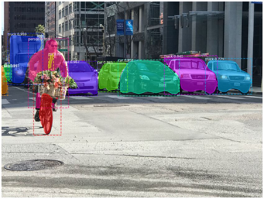
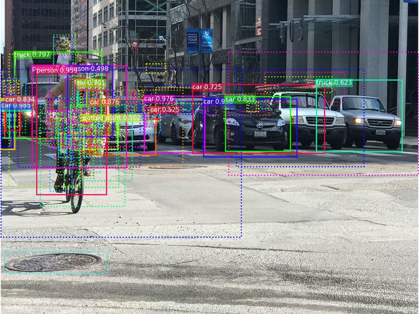
Instance Segmentation
• Obiettivo
 • Individuare non solo la segmentazione, ma anche l’istanza
Mask R-CNN
 • Mask R-CNN = Faster R-CNN + FCN sui RoIs

 Loss: )* + +,- + ./*0
Recap: Faster R-CNN
Da Faster R-CNN a Mask R-CNN
Mask R-CNN: Mask
• ⋅ ×
 • Una maschera di dimensione × per ognuna delle classi
 • Ogni pixel è regolato da una sigmoide
 • Loss
 • Su una RoI associata alla classe , %&'( è la binary cross-entropy relativa alla maschera
 ( associata
 • Le altre maschere non contribuiscono alla loss
Mask R-CNN
RoIAlign

• Il mapping di una regione sulla feature map con
 RoIPooling causa un riallineamento
RoIAlign
• Con RoIAlign, ogni punto viene interpolato
 • Recupera precision nella ricostruzione della maschera
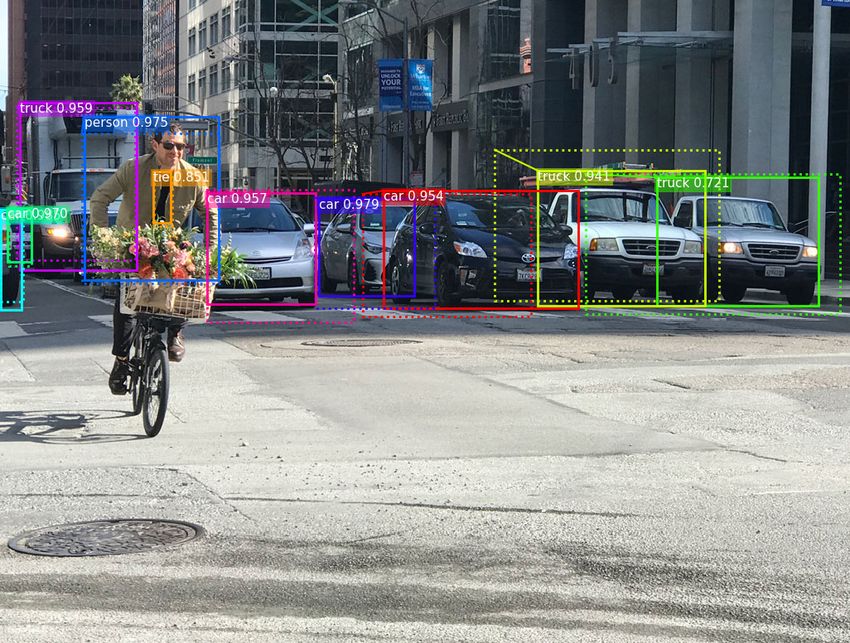
Risultati
• Priors
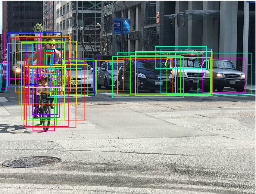
Risultati
• Region Proposals
Risultati
• Predizione
Risultati
• Non-Maximum Suppression
Risultati
• Mask
YOLOACT: You Only Look At CoefficienTs
• Due task paralleli:
 • Generazione di un dizionario di non-local prototype masks sull’intera
 immagine
 • Basato su FCN
 • Predizione di un insieme di coefficienti di combinazione per ogni istanza
 • Aggiunge una componente all’object detection per predire un vettore di “mask
 coefficients”
 • Per ogni istanza selezionata nel NMS viene costruita una maschera
 combinando i risultati dei due task. Feature Pyramid Mask Coefficients
 Detection 1 Detection 2
 Assembly

 Detection
 + + + + + - = 1
 Feature Backbone - -
 Person Racket
 Detection
 - + - + = 2

 Prediction
 NMS
 Head

 Crop Threshold

 Protonet

 Prototypes

 Figure 2: YOLACT Architecture Blue/yellow indicates low/high values in the prototypes, gray nodes indicate functions
 that are not trained, and k = 4 in this example. We base this architecture off of RetinaNet [27] using ResNet-101 + FPN.
Architettura

 Feature Pyramid Mask Coefficients Assembly
 Detection 1 Detection 2
 Detection
 + + + + + - = 1
 Feature Backbone - -
 Person Racket
 Detection
 - + - + = 2

 Prediction
 NMS
 Head

 Crop Threshold

 Protonet

 Prototypes

Figure 2: YOLACT Architecture Blue/yellow indicates low/high values in the prototypes, gray nodes indicate functions
that are not trained, and k = 4 in this example. We base this architecture off of RetinaNet [27] using ResNet-101 + FPN.

ture localization step (e.g., feature repooling). To do this, the computational overhead over that of the backbone de-
we break up the complex task of instance segmentation into tector comes mostly from the assembly step, 69×69
 69×69 which can be
 138×138 138×138 Cla W H
 P ×256 ×3 3
 ×256 ×256 × ca
two simpler, parallel tasks that can be assembled to form implemented as a single matrix multiplication. In this way, Cla W H W H W H
the final masks. The first branch uses an FCN [31] to pro- we can maintain spatial coherence in the feature space while 256 ×4 256 ca

duce a set of image-sized “prototype masks” that do not de- still being one-stage and fast. W H W H Bo W H
pend on any one instance. The second adds an extra head Figure 3: Protonet Architecture The labels denote fea- Pi Pi 256 256 4a

to the object detection branch to predict a vector of “mask 3.1. Prototype Generation Prototype FCN
 ture size and channels for an image size of 550 ⇥ 550. Ar-
 rows indicate 3 ⇥ 3 conv layers, except for the final conv
 W H
 256
 W H
 256
 W H
 4a
coefficients” for each anchor that encode an instance’s rep- The prototype generation branch (protonet) predicts a set Bo ×4

 which is 1 ⇥ 1. The increase in size is an upsample fol- W H
resentation in the prototype space. Finally, for each instance of k prototype masks forlowed
 the entire image. We implement Ma k ka
 by a conv. Inspired by the mask branch in [18].
that survives NMS, we construct a mask for that instance by protonet as an FCN whose last layer has k channels (one
 RetinaNet [27] Ours
Architettura

 Feature Pyramid Mask Coefficients Assembly
 Detection 1 Detection 2
 Detection
 + + + + + - = 1
 Feature Backbone - -
 Person Racket
 Detection
 - + - + = 2

 Prediction
 NMS
 Head

 Crop Threshold

 Protonet

 Prototypes
 69×69 69×69 138×138 138×138 Cla W H
 P3 ×256 ×3 ×256 ×256 × ca

Figure 2: YOLACT Architecture Blue/yellow indicates low/high values in the prototypes, gray nodes indicate functions Cla W H
 256 ×4
 W H
 256
 W H
 ca
that are not trained, and k = 4 in this example. We base this architecture off of RetinaNet [27] using ResNet-101 + FPN.
 W H W H Bo W H
 Figure 3: Protonet Architecture The labels denote fea- Pi Pi 256 256 4a

ture localization step (e.g., feature repooling). To do this, ture size and
 the computational channels
 overhead for that
 over an image sizebackbone
 of the of 550 ⇥ de-
 550. Ar- W H W H W H
we break up the complex task of instance segmentation into tector comes mostly from the assembly step, which can be conv
 rows indicate 3 ⇥ 3 conv layers, except for the final Bo
 256 ×4 256 4a
 which is 1 ⇥ 1. The increase in size is an upsample fol- W H
two simpler, parallel tasks that can be assembled to form implemented as a single matrix multiplication. In this way, Ma k ka
 lowed by a conv. Inspired by the mask branch in [18].
the final masks. The first branch uses an FCN [31] to pro- we can maintain spatial coherence in the feature space while
 RetinaNet [27] Ours
duce a set of image-sized “prototype masks” that do not de- still being sors.
 one-stage andcoefficient
 For mask fast. prediction, we simply add a third
pend on any one instance. The second adds an extra head Figure 4: Head Architecture We use a shallower predic-
 branch in parallel that predicts k mask coefficients, one cor-
to the object detection branch to predict a vector of “mask 3.1. Prototype Generation
 responding to each prototype. Thus, instead of producing
 tion head than RetinaNet [27] and add a mask coefficient
 branch. This is for c classes, a anchors for feature layer Pi ,
coefficients” for each anchor that encode an instance’s rep- 4 + c coefficients
 The prototype generation perbranch
 anchor,(protonet)
 we producepredicts
 4 + c +a k.
 set and k prototypes. See Figure 3 for a key.
resentation in the prototype space. Finally, for each instance Then
 of k prototype for nonlinearity,
 masks we image.
 for the entire find it important to be able to
 We implement
Architettura

 Feature Pyramid Mask Coefficients Assembly
 Detection 1 Detection 2
 Detection
 + + + + + - = 1
 Feature Backbone - -
 Person Racket

 = ( ⋅ 1 )
 Detection
 - + - + = 2

 Prediction
 Head
 NMS • matrice di maschere
 Crop Threshold
 • vettore di coefficienti
 Protonet

 Prototypes

Figure 2: YOLACT Architecture Blue/yellow indicates low/high values in the prototypes, gray nodes indicate functions
that are not trained, and k = 4 in this example. We base this architecture off of RetinaNet [27] using ResNet-101 + FPN.

ture localization step (e.g., feature repooling). To do this, the computational overhead over that of the backbone de-
we break up the complex task of instance segmentation into tector comes mostly from the assembly step, which can be
two simpler, parallel tasks that can be assembled to form implemented as a single matrix multiplication. In this way,
the final masks. The first branch uses an FCN [31] to pro- we can maintain spatial coherence in the feature space while
duce a set of image-sized “prototype masks” that do not de- still being one-stage and fast.
pend on any one instance. The second adds an extra head
to the object detection branch to predict a vector of “mask 3.1. Prototype Generation
coefficients” for each anchor that encode an instance’s rep- The prototype generation branch (protonet) predicts a set
resentation in the prototype space. Finally, for each instance of k prototype masks for the entire image. We implement
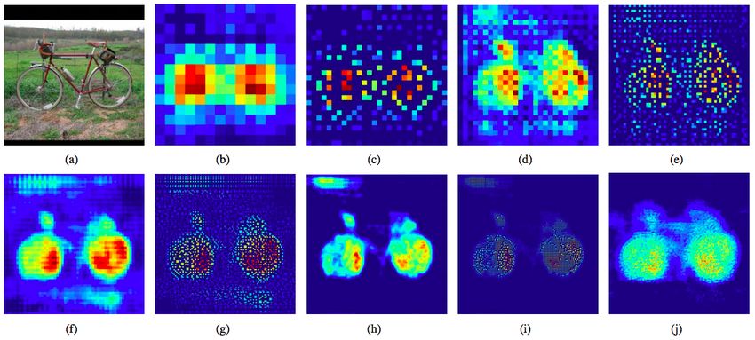
Caratteristiche
 co
 do
• Loss fol
 YO
 • -. + /01 + 23.4 [26
 • 23.4 = ( , 56 ) of
 ge
 we
• YOLACT impara a localizzare le istanze P7
 (no
 on
 an
 vio
 pre
 sha
 ow
 pre
 an
 gre
 wa
 cro
 Figure 5: Prototype Behavior The activations of the same sel
 six prototypes (y axis) across different images (x axis). Pro- ne
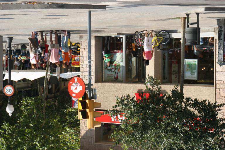
Risultati
• 29.8mAP, 33FPS

 Figure 6: YOLACT evaluation results on COCO’s test-dev set. This base model achieves 29.8 mAP at 33.0 fps. All
 images have the confidence threshold set to 0.3.
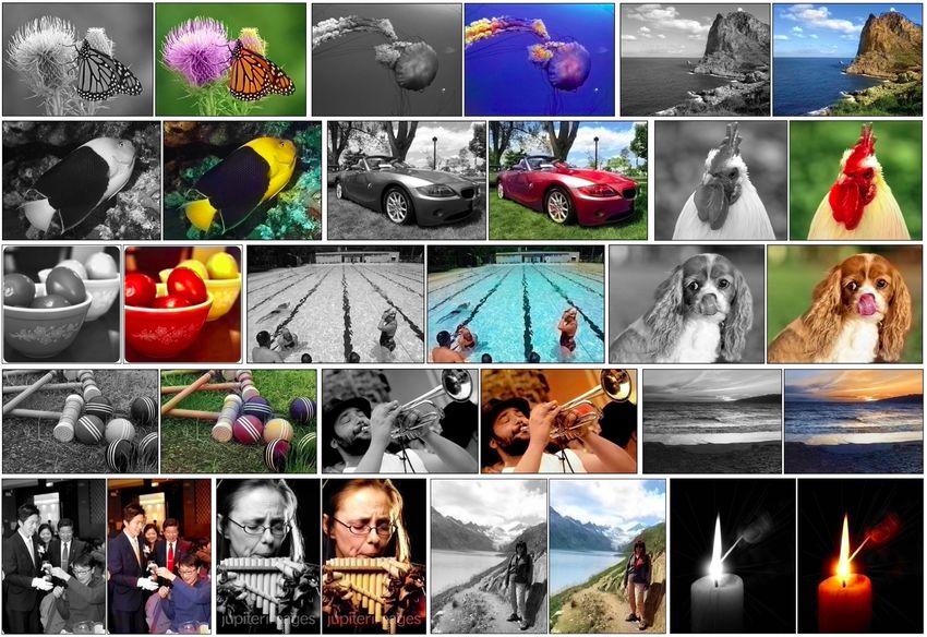
Riassunto
• Semantic vs. Instance segmentation
• Architetture complesse
• Base per learning task simili
 • Depth estimation
 • Surface normal estimation
 • Colorization
You can also read