An Introduction to Deep Morphological Networks - STORRE
←
→
Page content transcription
If your browser does not render page correctly, please read the page content below
Received July 15, 2021, accepted August 9, 2021, date of publication August 12, 2021, date of current version August 23, 2021.
Digital Object Identifier 10.1109/ACCESS.2021.3104405

An Introduction to Deep Morphological Networks
KEILLER NOGUEIRA 1,2 , JOCELYN CHANUSSOT 3 , (Fellow, IEEE),
MAURO DALLA MURA 4,5 , (Senior Member, IEEE),
AND JEFERSSON A. DOS SANTOS 1 , (Member, IEEE)
1 Department of Computer Science, Universidade Federal de Minas Gerais, Belo Horizonte 31270-901, Brazil
2 Computing Science and Mathematics, University of Stirling, Stirling FK9 4LA, U.K.
3 Inria,
       CNRS, Grenoble INP, LJK, University Grenoble Alpes, 38000 Grenoble, France
4 CNRS, Grenoble INP, GIPSA-Laboratory, University of Grenoble Alpes, 38000 Grenoble, France
5 Tokyo Tech World Research Hub Initiative (WRHI), School of Computing, Tokyo Institute of Technology, Tokyo 152-8550, Japan

Corresponding author: Keiller Nogueira (keiller.nogueira@stir.ac.uk)
This work was supported in part by the Minas Gerais Research Funding Foundation (FAPEMIG) under Grant APQ-00449-17, in part by the
National Council for Scientific and Technological Development (CNPq) under Grant 311395/2018-0 and Grant 424700/2018-2, and in part
by the Coordenação de Aperfeiçoamento de Pessoal de Nível Superior – Brasil (CAPES) – Finance Code 001 under Grant 88881.131682/
2016-01 and Grant 88881.145912/2017-01. We gratefully acknowledge the support of NVIDIA Corporation with the donation of the Titan
Xp GPU used for this research.

   ABSTRACT Over the past decade, Convolutional Networks (ConvNets) have renewed the perspectives of
   the research and industrial communities. Although this deep learning technique may be composed of multiple
   layers, its core operation is the convolution, an important linear filtering process. Easy and fast to implement,
   convolutions actually play a major role, not only in ConvNets, but in digital image processing and analysis
   as a whole, being effective for several tasks. However, aside from convolutions, researchers also proposed
   and developed non-linear filters, such as operators provided by mathematical morphology. Even though
   these are not so computationally efficient as the linear filters, in general, they are able to capture different
   patterns and tackle distinct problems when compared to the convolutions. In this paper, we propose a new
   paradigm for deep networks where convolutions are replaced by non-linear morphological filters. Aside from
   performing the operation, the proposed Deep Morphological Network (DeepMorphNet) is also able to learn
   the morphological filters (and consequently the features) based on the input data. While this process raises
   challenging issues regarding training and actual implementation, the proposed DeepMorphNet proves to be
   able to extract features and solve problems that traditional architectures with standard convolution filters
   cannot.

   INDEX TERMS Convolutional networks, deep learning, deep morphological networks, mathematical
   morphology.

I. INTRODUCTION                                                                                etc) and employed by several techniques (such as the filtering
Over the past decade, Convolutional Networks (ConvNet) [1]                                     approaches [10]).
have been a game changer in the computer vision community,                                        Aside from convolutions, researchers also proposed and
achieving state-of-the-art in several computer-vision appli-                                   developed non-linear filters, such as operators provided by
cations, including image classification [2], [3], object and                                   mathematical morphology. Even though these are not so
scene recognition [4]–[8], and many others. Although this                                      computationally efficient as the linear filters, in general,
deep learning technique may be composed of several dis-                                        they are able to capture different patterns and tackle dis-
tinct components (such as convolutional and pooling layers,                                    tinct problems when compared to the convolutions. For
non-linear activation functions, etc), its core operation is the                               instance, suppose one desires to preserve only the large
convolution, a linear filtering process whose weights, in this                                 objects of an input image with 4 × 4 and 2 × 2 squares.
case, are to be learned based on the input data. Easy and                                      As presented in Figure 1, despite having a myriad of pos-
fast to implement, convolutions actually play a major role,                                    sible configurations, the convolution is not able to pro-
not only in ConvNets [1], but in digital image processing                                      duce such an outcome that can be easily obtained, for
and analysis [9], [10] as a whole, being effective for many                                    example, by a non-linear morphological opening. In fact,
tasks (including image denoising [11], edge detection [12],                                    supported by this capacity of extracting distinct features,
                                                                                               some non-linear filters, such as the morphological opera-
    The associate editor coordinating the review of this manuscript and                        tions [13], are still very popular and state-of-the-art in some
approving it for publication was Geng-Ming Jiang             .                                 scenarios [14]–[17].

                     This work is licensed under a Creative Commons Attribution 4.0 License. For more information, see https://creativecommons.org/licenses/by/4.0/
114308                                                                                                                                                                VOLUME 9, 2021
K. Nogueira et al.: Introduction to DeepMorphNets

                                                                                  • a novel paradigm for deep networks where linear con-
                                                                                    volutions are replaced by the non-linear morphological
                                                                                    operations, and
                                                                                  • a technique, called Deep Morphological Network
                                                                                    (DeepMorphNet), capable of performing and optimiza-
                                                                                    tion morphological operations.
                                                                                  The remainder of this paper is organized as follows.
                                                                               Section II introduces some background concepts and presents
                                                                               the related work. The proposed method is presented
                                                                               in Section III. The experimental setup is introduced in
                                                                               Section IV while Section V presents the obtained results.
                                                                               Finally, Section VI concludes the paper.

                                                                               II. BACKGROUND KNOWLEDGE AND RELATED WORK
                                                                               This section introduces the basic principles underlying math-
                                                                               ematical morphology, and reviews the main approaches that
FIGURE 1. Illustration showing the lack of ability of the convolution filter   exploit such operations for distinct image tasks.
to produce certain outcomes that are easily generated by non-linear
operations. The goal here is to preserve only the larger squares of the
input image, as presented in the desired outcome. Towards such                 A. MATHEMATICAL MORPHOLOGY
objective, this image is processed by three distinct convolution filters       Morphological operations, commonly employed in the image
producing different outputs, none of them similar to the desired
outcome. However, a simple morphological opening with                          processing area, are strongly based on mathematical mor-
a 3 × 3 structuring element is capable of generating such output.              phology. Since its introduction to the image domain, these
                                                                               morphological operations have been generalized from the
                                                                               analysis of a single band image to hyperspectral images
   In this paper, we propose a novel paradigm for deep                         made up of hundreds of spectral channels and has become
networks where linear convolutions are replaced by the                         one of the state-of-the-art techniques for a wide range of
aforementioned non-linear morphological operations. Fur-                       applications [13]. This study area includes several different
thermore, differently from the current literature, wherein dis-                operations (such as erosion, dilation, opening, closing, top-
tinct morphological filters must be evaluated in order to find                 hats, and reconstruction), which can be applied to binary and
the most suitable ones for each application, the proposed                      grayscale images in any number of dimensions [13].
technique, called Deep Morphological Network (DeepMor-                            Formally, consider a grayscale 2D image I (·) as a mapping
phNet), learns the filters (and consequently the features)                     from the coordinates (Z2 ) to the pixel-value domain (Z).
based on the input data. Technically, the processing of each                   Most morphological transformations process this input
layer of the proposed approach can be divided into three                       image I using a structuring element (SE) (usually defined
steps/operations: (i) depthwise convolution [18], employed                     prior to the operation). A flat1 SE B(·) can be defined as a
to rearrange the input pixels according to the binary fil-                     function that, based on its format (or shape), returns a set of
ters, (ii) depthwise pooling, used to select some pixels and                   neighbors of a pixel (i, j). This neighborhood of pixels is taken
generate an eroded or dilated outcome, and (iii) pointwise                     into account during the morphological operation, i.e., while
convolution [18], employed to combine the generated maps                       probing the image I . As introduced, the definition of the SE is
producing one final morphological map (per neuron). This                       of vital importance for the process to extract relevant features.
process resembles the depthwise separable convolutions [18]                    However, in literature [19], [20], this definition is performed
but using binary filters and one more step (the second one)                    experimentally (with common shapes being squares, disks,
between the convolutions. Note that, to the best of our                        diamonds, crosses, and x-shapes), an expensive process that
knowledge, this is the first proof of concept work related to                  does not guarantee a good descriptive representation.
networks capable of performing and optimizing exact (non-                         After its definition, the SE can be then employed in sev-
approximate) morphological operations with flat structur-                      eral morphological processes. Most of these operations are
ing elements (i.e., filters). Particularly, this is an advantage               usually supported by two basic morphological transforma-
given that the vast majority of the mathematical morphol-                      tions: erosion E(·) and dilation δ(·). Such operations receive
ogy operators based on structuring elements employ flat                        basically the same input: an image I and the SE B. While
filters. While this replacement process raises challenging                     erosion transformations process each pixel (i, j) using the
issues regarding training and actual implementation, the pro-                  supremum function ∧, as denoted in Equation 1, the dilation
posed DeepMorphNet proves to be able to solve problems                         operations process the pixels using the infimum ∨ function,
that traditional architectures with standard convolution filters               as presented in Equation 2. Intuitively, these two operations
cannot.                                                                          1 A flat SE is binary and only defines which pixels of the neighborhood
   In practice, we can summarize the main contributions of                     should be taken into account. On the other hand, a non-flat SE contains finite
this paper as follows:                                                         values used as additive offsets in the morphological computation.

VOLUME 9, 2021                                                                                                                                       114309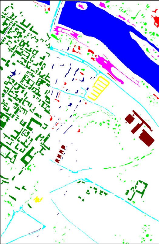
K. Nogueira et al.: Introduction to DeepMorphNets

probe an input image using the SE, i.e., they position the
structuring element at all possible locations in the image
and analyze the neighborhood pixels. This process, somehow
similar to the convolution procedure, outputs another image
with regions compressed or expanded. Some examples of
erosion and dilation are presented in Figure 2, in which it
is possible to notice the behavior of each operation. As can
be noticed erosion affects brighter structures while dilation
influences darker ones (w.r.t. the neighborhood defined by
the SE).
         E(B, I )(i,j) = {∧I ((i, j)0 )|(i, j)0 ∈ B(i, j) ∪ I (i, j)}   (1)
         δ(B, I )(i,j) = {∨I ((i, j)0 )|(i, j)0 ∈ B(i, j) ∪ I (i, j)}   (2)
                                                                              FIGURE 2. Examples of morphological images generated for the
                                                                              UCMerced Land-use Dataset. For better viewing and understanding,
   If we have an ordered set, then the erosion and dilation                   images (b)-(j) only present a left-bottom zoom of the original image (a).
operations can be simplified. This is because the infimum and                 All these images were processed using a 5 × 5 square as structuring
the supremum are respectively equivalent to the minimum                       element.

and maximum functions when dealing with ordered sets.
In this case, erosion and dilation can be defined as presented
                                                                              opening is calculated, and (ii) the black one, denoted as T b (·)
in Equations 3 and 4, respectively.
                                                                              and defined in Equation 8, in which the difference between
                 E(B, I )(i,j) = { min
                                   0
                                       (I ((i, j)0 ))}                  (3)   the closing and the input image is performed. White top-hat
                                    (i,j) ∈B(i,j)                             operation preserves elements of the input image brighter than
                  δ(B, I )(i,j) = { max (I ((i, j)0 ))}                 (4)   their surroundings but smaller than the SE. On the other hand,
                                    (i,j)0 ∈B(i,j)
                                                                              black top-hat maintains objects smaller than the SE with
   Based on these two fundamental transformations, other                      brighter surroundings. Examples of these two operations can
more complex morphological operations may be computed.                        be seen in Figure 2.
The morphological opening, denoted as γ (·) and defined in
Equation 5, is simply an erosion operation followed by the                                          T w (B, I ) = I − γ (B, I )                      (7)
dilation (using the same SE). In contrast, a morphological                                          T b (B, I ) = ϕ(B, I ) − I                       (8)
closing ϕ(·) of an image, defined in Equation 6, is a dilation
                                                                                 Another important morphological operation based on ero-
followed by the erosion (using the same SE). Intuitively,
                                                                              sions and dilations is the geodesic reconstruction. There
an opening flattens bright objects that are smaller than the
                                                                              are two types of geodesic reconstruction: by erosion and
size of the SE and, because of dilation, mostly preserves the
                                                                              by dilation. The geodesic reconstruction by erosion ρ E (·),
bright large areas. A similar conclusion can be drawn for
                                                                              mathematically defined in Equation 9, receives two param-
darker structures when closing is performed. Examples of
                                                                              eters as input: an image I and a SE B. The image I (also
this behavior can be seen in Figure 2. It is important to
                                                                              referenced in this operation as mask image) is dilated by
highlight that by using erosion and dilation transformations,
                                                                              the SE B (δ(B, I )) creating the marker image Y (Y ∈ I ),
opening and closing perform geodesic reconstruction in the
                                                                              responsible for delimiting which objects will be reconstructed
image. Operations based on this paradigm belongs to the class
                                                                              during the process. A SE B0 (usually with any elementary
of filters that operate only on connected components (flat
                                                                              composition [13]) and the marker image Y are provided
regions) and cannot introduce any new edge to the image.
                                                                              for the reconstruction operation REI (·). This transformation,
Furthermore, if a segment (or component) in the image is
                                                                              defined in Equation 10, reconstructs the marker image Y
larger than the SE then it will be unaffected, otherwise,
                                                                              (with respect to the mask image I ) by recursively employing
it will be merged to a brighter or darker adjacent region
                                                                              geodesic erosion (with the elementary SE B0 ) until idem-
depending upon whether a closing or opening is applied.                                                   (n)         (n+1)
This process is crucial because it avoids the generation                      potence is reached (i.e., EI (·) = EI         (·)). In this case,
                                                                                                    (1)
of distorted structures, which is obviously an undesirable                    a geodesic erosion EI (·), defined in Equation 11, consists
effect.                                                                       of a pixel-wise maximum operation between an eroded (with
                                                                              elementary SE B0 ) marker image Y and the mask image I .
                        γ (B, I ) = δ(B, E(B, I ))                      (5)   By duality, a geodesic reconstruction by dilation can be
                        ϕ(B, I ) = E(B, δ(B, I ))                       (6)   defined, as presented in Equation 12. These two crucial
                                                                              operations try to preserve all large (than the SE) objects
   Other important morphological operations are the top-hats.
                                                                              of the image removing bright and dark small areas, such
Top-hat transform is an operation that extracts small elements
                                                                              as noises. Some examples of these operations can be seen
and details from given images. There are two types of top-hat
                                                                              in Figure 2.
transformations: (i) the white one T w (·), defined in Equa-
tion 7, in which the difference between the input image and its                  ρ E (B, I ) = REI (B0 , Y ) = REI (B0 , δ(B, I ))                   (9)

114310                                                                                                                                    VOLUME 9, 2021
K. Nogueira et al.: Introduction to DeepMorphNets

                    (n)
 REI (B0 , Y ) = EI (B0 , Y )                                      morphological operations. In fact, several works [20], [25],
                                                                   [26], [28] tried to combine these techniques to create a more

                   (1)       (1)         (1) 0 (1) 0
               = EI B , EI B , · · · EI B , EI (B , Y )
                         0         0
                                                                   robust model. Some works [20], [28] employed morphologi-
                 |                      {z                 }       cal operations as a pre-processing step in order to extract the
                                     n times                       first set of discriminative features. In these cases, pre-defined
                                                         (10)      (hand-crafted) structuring elements are employed. Those
  (1) 0
 EI (B , Y ) = max{E(B , Y ), I }
                           0
                                                         (11)      techniques use such features as input for a ConvNet respon-
    ρ δ (B, I ) = RδI (B0 , Y ) = RδI (B0 , E(B, I ))      (12)    sible to perform the classification. Based on the fact that
                                                                   morphology generates interesting features that are not cap-
   Note that geodesic reconstruction operations require an         tured by the convolutional networks, such works achieved
iterative process until the convergence. This procedure can        outstanding results on pixelwise classification.
be expensive, mainly when working with a large number of              Other works [23]–[26] introduced morphological opera-
images. An approximation of such operations, presented in          tions into neural networks, creating a framework in which
Equations 13 and 14, can be achieved by performing just            the structuring elements are optimized. Masci et al. [25]
one transformation over the marker image with a large (than        proposed a convolutional network that aggregates pseudo-
the SE used to create the marker image) structuring element.       morphological operations. Specifically, their proposed
In other words, suppose that B is the SE used to create the        approach uses the counter-harmonic mean, which allows the
marker image, then B0 , the SE used in the reconstruction          convolutional layer to perform its traditional linear process,
step, should be larger than B. This process is faster since        or approximations of morphological operations. They show
only one iteration is required, but may lead to worse results,     that the approach produces outcomes very similar to real
given that the use of a large filter can make the reconstruction   morphological operations. Mellouli et al. [26] performed a
join objects that are close in the scene (a phenomenon known       more extensive validation of the previous method, proposing
as leaking [13]).                                                  different deeper networks that are used to perform image
                                                                   classification. In their experiments, the proposed network
                     ρ̃ E (B, I ) = EI (B0 , δ(B, I ))     (13)    achieved promising results for two datasets of digit recog-
                      ρ̃ δ (B, I ) = δI (B0 , E(B, I ))    (14)    nition. In [23], the authors proposed a new network capable
                                                                   of performing some morphological operations (including
B. RELATED WORK                                                    erosion, dilation, opening, and closing) while optimizing
As introduced, such non-linear morphological opera-                non-flat structuring elements. Their proposed network, eval-
tions [13] have the ability to preserve some features that         uated for image de-raining and de-hazing, produced results
may be essential for some problems. Supported by this,             similar to those of a ConvNet but using much fewer parame-
several tasks and applications have exploited the benefits of      ters. Finally, Franchi et al. [24] proposed a new deep learning
morphological operations, such as image analysis [16], [17],       framework capable of performing non-approximated mathe-
[21]–[24], classification [25]–[27], segmentation [14], [15],      matical morphology operations (including erosion, dilation)
[20], [28], [29], and so on.                                       while optimizing non-flat structuring elements. Their method
   Some of these techniques [16], [21], [22], [29] are strongly    produced competitive results for edge detection and image
based on mathematical morphology. These approaches pro-            denoising when compared to classical techniques and stan-
cess the input images using only morphological operations.         dard ConvNets.
The produced outcomes are then analyzed in order to extract           In this work, we proposed a new network capable of per-
high-level semantic information, such as borders, area,            forming and optimizing several morphological operations,
geometry, volume, and more. Other works [14], [15], [17],          including erosion, dilation, openings, closing, top-hats, and
[19], [27] go further and use morphology to extract robust         an approximation of geodesic reconstructions. Several dif-
features that are employed as input to machine learning tech-      ferences may be pointed out between the proposed approach
niques (such as Support Vector Machines, and decision trees)       and the aforementioned works: (i) differently from [25], [26],
to perform image analysis, classification, and segmentation.       the proposed technique really carries out morphological oper-
Usually, in these cases, the input images are processed using      ations without any approximation (except for the reconstruc-
several different morphological transformations, each one          tion), (ii) the morphological operations incorporated into the
employing a distinct structuring element, in order to improve      proposed network use flat SEs (which may be used with
the diversity of the extracted features. All these features are    any input image), thus differing from other methods, such
then concatenated and used as input for the machine learning       as [23], [24], that can only optimize morphological operations
techniques.                                                        using non-flat SEs and, consequently, can only be used with
   More recently, ConvNets [1] started achieving outstand-         grayscale input data, and (iii) to the best of our knowledge,
ing results, mainly in applications related to images. There-      this is the first approach to implement (approximate) morpho-
fore, it would be more than natural for researchers to             logical geodesic reconstruction within deep-learning based
propose works combining the benefits of ConvNets and               models.

VOLUME 9, 2021                                                                                                               114311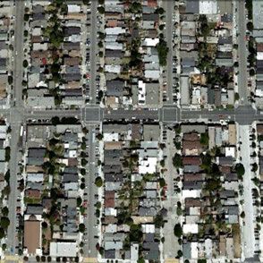
K. Nogueira et al.: Introduction to DeepMorphNets

III. DEEP MORPHOLOGICAL NETWORKS                                  is presented in Section III-A. This concept is employed
In this section, we present the proposed approach, called         to create morphological neurons and layers, presented in
Deep Morphological Networks (or simply DeepMorphNets),            Sections III-B and III-C, respectively. Section III-D explains
that replaces the linear convolutional filters with optimiz-      the optimization processed performed to learn the structure
able non-linear morphological operations. Such replacement        elements. Finally, the morphological architecture exploited in
allows the proposed network to capture distinct information       this work are introduced in Section III-E.
when compared to previous existing models, an advantage
that may assist different applications. However, this process     A. BASIC MORPHOLOGICAL FRAMEWORK
raises several challenging issues.                                Towards the preservation of the end-to-end learning strategy,
   One first challenge is due to the linear nature of the core    we propose a new framework, capable of performing mor-
operations of the existing networks. The convolutional layers     phological erosion and dilation, that uses operations already
extract features from the input data using an optimizable         employed in other existing deep learning-based methods. The
filter by performing only linear operations not supporting        processing of this framework can be separated into two steps.
non-linear ones. Formally, let us assume a 3D input y(·) of       The first one employs depthwise convolution [18] to perform
a convolutional layer as a mapping from coordinates (Z3 )         a delimitation of features, based on the neighborhood (or
to the pixel-value domain (Z or R). Analogously, the train-       filter). As defined in Equation 17, this type of convolution
able filter (or weight) W (·) of such layer can be seen as        differs from standard ones since it handles the input depth
a mapping from 3D coordinates (Z3 ) to the real-valued            independently, using the same filter W to every input channel.
weights (R). A standard convolutional layer performs a            In other words, suppose that a layer performing depthwise
convolution of the filter W (·) over the input y(·), accord-      convolution has k filters and receives an input with l chan-
ing to Equation 15. Note that the output of this operation        nels, then the processed outcome would be an image of
is the summation of the linear combination between input          k × l channels, since each k-th filter would be applied to
and filter (across both space and depth). Also, observe the       each l-th input channel. The use of depthwise convolution
difference between this operation and the morphological           simplifies the introduction of morphological operations into
ones stated in Section II-A. This shows that replacing the        the deep network since the linear combination performed by
convolutional filters with morphological operations is not        this convolution does not consider the depth (as in standard
straightforward.                                                  convolutions presented in Equation 15). This process is fun-
                  XXX                                             damental for the recreation of morphological operations since
  S(W , y)(i,j) =            W (m, n, l)y(i+m, j+n, l) (15)
                 m    n
                                                                  such transformations can only process one single channel at
                          l
                                                                  a time.
   Another important challenge is due to the optimization of                               XX
non-linear operations by the network. Precisely, in ConvNets,            Sl (W , y)(i,j) =     W (m, n)y(i + m, j + n, l) (17)
a loss function L is used to optimize the model. Neverthe-                              m    n
less, the objective of any network is to minimize this loss          However, just using this type of convolution does not allow
function by adjusting the trainable parameters (or filters) W .   the reproduction of morphological transformations, given
Such optimization is traditionally based on the derivatives       that a spatial linear combination is still performed by this
of the loss function L with respect to the weights W . For        convolutional operation. To overcome this, all filters W are
instance, suppose Stochastic Gradient Descent (SGD) [1] is        first converted into binary and then used in the depthwise
used to optimize a ConvNet. As presented in Equation 16,          convolution operation. This binarization process, referenced
the optimization of the filters depends directly on the par-      hereafter as max-binarize, activates only the highest value of
tial derivatives of the loss function L with respect to the       the filter. Formally, the max-binarize b(·) is a function that
weights W (employed with a pre-defined learning rate α).          receives as input the real-valued weights W and processes
Those partial derivatives are usually obtained using the back-    them according to Equation 18, where 1{condition} is the
propagation algorithm [1], which is strongly supported by         indicator function. This process outputs a binary version of
the fact that all operations of the network are easily dif-       the weights, W b , in which only the highest value in W is acti-
ferentiable, including the convolution presented in Equa-         vated in W b . By using W b , the linear combination performed
tion 15. However, this algorithm cannot be directly applied       by depthwise convolution can be seen as a simple operation
to non-linear operations, such as the presented morpho-           that preserves the exact value of the single pixel activated by
logical ones, because those operations do not have easy           this binary filter.
derivatives.                                                         b
                                    ∂L                             W(i,j) = b(W (i, j)) = 1{maxm,n (W (m, n)) = W (i, j)} (18)
                      W =W −α                             (16)
                                   ∂W                                But preserving only one pixel with respect to the binary fil-
   Overcoming such challenges, we propose a network               ter is not enough to reproduce the morphological operations,
that employs depthwise and pointwise convolution with             since they usually operate over a neighborhood (defined by
depthwise pooling to recreate and optimize morphological          the SE B). In order to reproduce this neighborhood concept
operations. The basic concepts of the proposed technique          in the depthwise convolution operation, we decompose each

114312                                                                                                                    VOLUME 9, 2021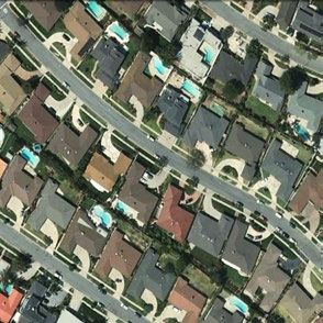
K. Nogueira et al.: Introduction to DeepMorphNets

filter W into several ones, that when superimposed retrieve
the final SE B. More specifically, suppose a filter W with
size s × s. Since only one position can be activated at a time,
this filter has a total of s2 possible activation variations. This
analysis is the same if we consider each element of a s × s SE
independently. Based on all this, a set of s2 max-binary filters
with size s × s is able to cover all possible configurations of
a SE with the same size. Thus, a set of s2 filters with size
s × s can be seen as a decomposed representation of the struc-
turing element, given that those s2 filters (with only a single
activated position) can be superimposed in order to retrieve
any possible s × s neighborhood configuration defined by the
SE. By doing this, the concept of neighborhood introduced
by the SE can be exploited by the depthwise convolution.
Technically, a s2 set of s × s filters W can be converted into
binary weights W b and then, used to process the input data.
When exploited by Equation 17, each of these s2 binary filter        FIGURE 3. Example of a morphological erosion based on the proposed
                                                                     framework. The 4 filters W (with size 4 × 4) actually represent a unique
W b will preserve only one pixel which is directly related           4 × 4 SE. Each filter W is first converted to binary W b , and then used to
to one specific position of the neighborhood. As may be              process each input channel (step 1, blue dashed rectangle). The output is
observed, this first step recreates, in depth, the neighborhood      then processed via a pixel and depthwise min-pooling to produce the
                                                                     final eroded output (step 2, green dotted rectangle). Note that the binary
of a pixel delimited by a s × s SE B, which is essentially           filters W b , when superimposed, retrieve the final SE B. The dotted line
represented by s2 binary filters W b of size s × s.                  shows that the processing of the input with the superimposed SE B using
                                                                     the standard morphological erosion results in the same eroded output
   Since the SE B was decomposed in depth, in order to               image produced by the proposed morphological erosion.
retrieve it, a depthwise operation must be performed over the
s2 binary filters W b . Analogously, a depthwise operation is
also required to retrieve the final outcome, i.e., the eroded        maximum operations also operate over the channels.
or dilated image. This is the second step of this proposed
                                                                       M E (W , y)(i,j) = PE (Sl (W , y))(i,j) = min Sl (W , y)(i,j)       (21)
framework, which is responsible to extract the relevant infor-                                                        l
mation based on the depthwise neighborhood. In this step,              M δ (W , y)(i,j) = Pδ (Sl (W , y))(i,j) = max Sl (W , y)(i,j)       (22)
an operation, called depthwise pooling P(·), processes the                                                            l
s2 outcomes (of the decomposed filters), producing the final            A visual example of the proposed framework being used
morphological outcome. This pooling operation is able to             for morphological erosion is presented in Figure 3. In this
actually output the morphological erosion and dilation by            example, the depthwise convolution has 4 filters W with size
using pixel and depthwise minimum and maximum functions,             4 × 4 which actually represent a unique 4 × 4 SE. The filters
as presented in Equations 19 and 20, respectively. The out-          W are first converted into binary using the max-binarize
come of this second step is the final (eroded or dilated) feature    function b(·), presented in Equation 18. Then, each binary
map that will be exploited by any subsequent process.                filter W b is used to process (step 1, blue dashed rectangle)
                                                                     each input channel (which, for simplicity, is only one in this
                      PE (y)(i,j) = min y(i, j, l)           (19)    example) using Equation 17. In this process, each binary
                                       l
                      Pδ (y)(i,j) = max y(i, j, l)           (20)    filter W b outputs an image in which each pixel has a direct
                                        l                            connection to the one position activated in that filter. The
   Equations 21 and 22 compile the two steps performed               output is then processed (step 2, green dotted rectangle)
by the proposed framework for morphological erosion and              via a pixel and depthwise min-pooling P(·)E (according to
dilation, respectively. This operation, denoted here as M (·),       Equation 19) to produce the final eroded output. Note that
performs a depthwise convolution (first step), which uses            the binary filters W b , when superimposed retrieve the final
max-binary filters that decompose the representation of the          SE B. The dotted line shows that the processing of the input
neighborhood concept introduced by SEs, followed by a pixel          with the superimposed SE B using the standard erosion (E(·)
and depthwise pooling operation (second step), outputting the        presented in Equation 3) results in the same eroded output
final morphological (eroded or dilated) feature maps. Note           image produced by the proposed morphological erosion.
the similarity between these functions and Equations 3 and 4
presented in Section II-A. The main difference between these         B. MORPHOLOGICAL PROCESSING UNITS
equations is in the neighborhood definition. While in the            The presented framework is the foundation of all proposed
standard morphology, the neighborhood of a pixel is defined          morphological processing units (or neurons). Before pre-
spatially (via SE B), in the proposed framework, the neighbor-       senting them, it is important to observe that, although the
hood is defined along the channels due to the decomposition          proposed framework is able to reproduce morphological ero-
of the SE B into several filters and, therefore, minimum and         sion and dilation, it has an important drawback: since it

VOLUME 9, 2021                                                                                                                          114313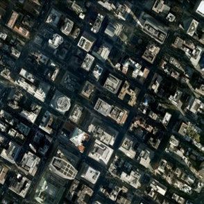
K. Nogueira et al.: Introduction to DeepMorphNets

employs depthwise convolution, the number of outcomes can          i.e., the same SE B. Equations 25 and 26 define the opening
grow potentially, given that, each input channel is processed      and closing morphological neurons, respectively. Note the
independently by each processing unit. In order to overcome        similarity between these functions and Equations 5 and 6.
this issue and make the proposed technique more scalable,
we propose to use a pointwise convolution [18] to force each                      M γ (W , y) = M δ (W , M E (W , y))                      (25)
processing unit to output only one image (or feature map).                        M ϕ (W , y) = M E (W , M δ (W , y))                      (26)
Particularly, all neurons proposed in this work have the same
design with two parts: (i) the core operation (fundamentally       3) TOP-HAT PROCESSING UNITS
based on the proposed framework), in which the processing          The implementation of other, more complex, morphological
unit performs its morphological transformation outputting          operations is a little more tricky. This is the case of the top-hat
multiple outcomes, and (ii) the pointwise convolution [18],        operations, which require both the input and processed data
which performs a pixel and depthwise (linear) combination          to generate the final outcome. Therefore, for such opera-
of the outputs producing only one outcome. Observe that,           tions, a skip connection [1] (based on the identity mapping)
even though the pointwise convolution performs a depthwise         is employed to support the forwarding of the input data,
combination of the multiple outcomes, it does not learn any        allowing it to be further processed. The core of the top-hat
spatial feature, since it employs a pixelwise (or pointwise)       processing units is composed of three parts: (i) an opening
operation, managing each pixel separately. This design allows      or closing morphological processing unit, depending on the
the morphological neuron to have the exact same input and          type of the top-hat, (ii) a skip connection, that allows the for-
output of a standard existing processing unit, i.e., it receives   warding of the input data, and (iii) a subtraction function that
as input an image with any number of bands and outputs a           operates over the data of both previous parts, generating the
single new representation. It is interesting to notice that this   final outcome. Such operation and its counterpart (the black
processing unit design employs depthwise and pointwise con-        top-hat) are defined in Equations 27 and 28, respectively.
volution [18], resembling very much the depthwise separable
                                                                                    M T (W , y) = y − M γ (W , y)
                                                                                            w
convolutions [18], but with extra steps and binary decom-                                                                                  (27)
posed filters. Next Sections explain the core operation of all                             Tb                 ϕ
                                                                                    M           (W , y) = M (W , y) − y                    (28)
proposed morphological processing units. Note that, although
not mentioned in the next Sections, the pointwise convolution      4) GEODESIC RECONSTRUCTION PROCESSING UNITS
is present in all processing units as aforementioned.
                                                                   Similarly to the previous processing units, the geodesic
                                                                   reconstruction also requires the input and processed data
1) COMPOSED PROCESSING UNITS
                                                                   in order to produce the final outcome. Hence, the imple-
The first morphological neurons, called composed processing        mentation of this important operation is also based on skip
units, have, in their core, a morphological erosion followed       connections. Aside from this, as presented in Section II-A,
by a dilation (or vice-versa), without any constraint on the       reconstruction operations require an iterative process.
weights. The motivation behind the composed processing             Although this procedure is capable of producing better out-
unit is based on the potential of the learned representation.      comes, its introduction in a deep network is not straightfor-
While erosion and dilation can learn simple representations,       ward, given that each process can take a different number of
the combination of these operations is able to capture more        iterations. Supported by this, the reconstruction processing
complex information. Equations 23 and 24 present the two           units proposed in this work are an approximation, in which
possible configurations of the morphological composed neu-         just one transformation over the marker image is performed.
rons. It is important to notice that the weights (W1 and W2 ) of   Based on this, the input is processed by two basic morpho-
each operation of this neuron are independent.                     logical operations (without any iteration) and an elementwise
             M Cδ (W , y) = M δ (W2 , M E (W1 , y))        (23)    max- or min-operation (depending on the reconstruction) is
                                                                   performed over the input and processed images. Such concept
             M CE (W , y) = M E (W2 , M δ (W1 , y))        (24)
                                                                   is presented in Equations 29 and 30 for reconstruction by
                                                                   erosion and dilation, respectively. Note that the SE used in the
2) OPENING AND CLOSING PROCESSING UNITS
                                                                   reconstruction of the marker image (denoted in Section II-A
The proposed framework is also able to support the imple-
                                                                   by B0 ) is a dilated version of the SE employed to create such
mentation of more complex morphological operations. The
                                                                   image.
most intuitive and simple transformations to be implemented
                                                                                     E
are the opening and closing (presented in Section II-A).                         M ρ̃ (W , y) = MyE (W , M δ (W , y))                      (29)
In fact, the implementation of the opening and closing pro-
                                                                                    ρ̃ δ
cessing units, using the proposed framework, is straightfor-                      M (W , y) = Myδ (W , M E (W , y))                        (30)
ward. The core of such neurons is very similar to that of
the composed processing units, except that in this case a          C. MORPHOLOGICAL LAYER
tie on the filters of the two basic morphological operations       After defining the processing units, we are able to specify
is required in order to make them use the same weights,            the morphological layers, which provide the essential tools

114314                                                                                                                            VOLUME 9, 2021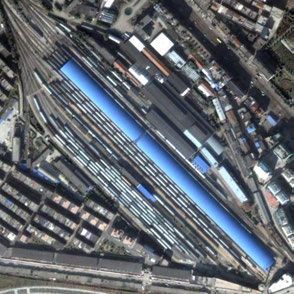
K. Nogueira et al.: Introduction to DeepMorphNets

for the creation of the DeepMorphNets. Similar to the stan-         pointwise convolution. The first part (of line 16) propagates
dard convolutional layer, this one is composed of several           the error of a specific pointwise convolution to the previous
processing units. However, the proposed morphological layer         operation, while the second part calculates the error of that
has two main differences when conceptually compared to              specific pointwise convolution operation. The same process
the convolutional one. The first one is related to the neurons      is repeated for the second and then for the first depthwise
that compose the layers. Particularly, in convolutional layers,     convolutions (lines 13 and 14, respectively). Note that during
the neurons are able to perform the convolution operation.          the backpropagation, the depthwise pooling is not optimized
Though the filter of each neuron can be different, the oper-        since this operation has no parameters and only passes the
ation performed by each processing unit in a convolutional          gradients to the previous layer. The last step of the training
layer is a simple convolution. On the other hand, there are sev-    process is the update of the weights and optimization of the
eral types of morphological processing units, from opening          network. This process is comprised in the loop from line
and closing to geodesic reconstruction. Therefore, a single         17 to 21. For a specific layer, line 18 updates the weights of
morphological layer can be composed of several neurons              the pointwise convolution while lines 19 and 20 update the
that may be performing different operations. This process           parameters of the first and second depthwise convolutions,
allows the layer to produce distinct (and possibly comple-          respectively.
mentary) outputs, increasing the heterogeneity of the network
and, consequently, the generalization capacity. The second          Algorithm 1 Training a Deep Morphological Network With
difference is the absence of activation functions. More specif-     L Layers
ically, in modern architectures, convolutional layers are usu-      Require: a minibatch of inputs and targets (y0 , y∗ ), previous
ally composed of a convolution operation followed by an                 weights W , and previous learning rate α.
activation function (such as ReLU [30]), that explicitly maps       Ensure: updated weights W .
the data into a non-linear space. In morphological layers,           1: 1. Forward propagation:
there are only processing units and no activation function is        2: for k=1 to L do
employed.                                                            3:    {First Processing Unit Operation}
                                                                                (1)          (1)
                                                                     4:    Wkb ← b(Wk )
D. OPTIMIZATION                                                             (1)                    (1)
                                                                     5:    sk ← yk−1 ∗ Wkb
Aside from defining the morphological layer, as introduced,                 (1)          (1)
                                                                     6:    yk ← P(sk )
we want to optimize its parameters, i.e., the filters W . Since
                                                                     7:    {Second Processing Unit Operation}
the proposed morphological layer uses common (differen-                         (2)          (2)
                                                                     8:    Wkb ← b(Wk )
tiable) operations already employed in other existing deep                  (2)      (1)         (2)
learning-based methods, the optimization of the filters is           9:    sk ← yk ∗ Wkb
                                                                            (2)          (2)
straightforward. In fact, the same traditional existing tech-       10:    yk ← P(sk )
                                                                                    (2)       (1×1)
niques employed in the training of any deep learning-based          11:    yk ← yk ∗ Wk                 {Pointwise Convolution}
approach, such feedforward, backpropagation and SGD [1],            12: end for
can also be used for optimizing a network composed of               13: 2. Backpropagation: {Gradients are not binary.}
                                                                                               ∂L
morphological layers.                                               14: Compute g (1) = ∂y knowing yL and y∗
                                                                                     yL          L
   The training procedure is detailed in Algorithm 1. Given         15: for k=L to 1 do
the training data (y0 , y∗ ), the first step is the feedforward,    16:
                                                                                               (1×1)         |
                                                                           gyk−1 ← gy(1) Wk−1 , gW (1×1) ← g (1) yk−1
                                                                                        k                    k−1           yk
comprised in the loop from line 2 to 8. In the first part                                     (2)
                                                                                           b ,g                        |        (2)
of line 4, the weights of the first depthwise convolution           17:     gy(2) ← gyk−1 Wk−1          b    (2)   ← gyk−1 yk−1
                                                                              k−1                      Wk−1
                                                                                              (1)                      |     (1)
are converted into binary (according to Equation 18). Then,                                b ,g
                                                                            gy(1) ← gy(2) Wk−1                     ←g
                                                                    18:                                 b    (1)        (2) y
in the second part, the first depthwise convolution (denoted                  k−1       k−1            Wk−1            yk−1 k−1
here as ∗) is performed, with the first depthwise pooling being     19:   end for
executed in the third part of this line. The same operations        20:   3. Update the weights:
are repeated in line 6 for the second depthwise convolution         21:   for k=1 to L do
                                                                               (1×1)      (1×1)
and pooling. Finally, in line 7, the pointwise convolution is       22:      Wk      ← Wk       − αgW (1×1)
                                                                                                              k
                                                                               (1)      (1)
carried out. After the forward propagation, the total error of      23:     Wk       ← Wk − αg         (1)
                                                                                                    Wkb
the network can be estimated. With this error, the gradients                   (2)      (2)
                                                                    24:     Wk ← Wk − αg b(2)
of the last layer can be directly estimated (line 10). These                            Wk
gradients can be used by the backpropagation algorithm to           25:   end for
calculate the gradients of the inner layers. In fact, this is the
process performed in the second training step, comprised in
the loop from line 11 to 15. It is important to highlight that      E. DeepMorphNet ARCHITECTURES
during the backpropagation process, the gradients are calcu-        Two networks, composed essentially of morphological and
lated normally, using real-valued numbers (and not binary).         fully connected layers, were proposed for the image and pixel
Precisely, line 12 is responsible for the optimization of the       classification tasks. Although such architectures have distinct

VOLUME 9, 2021                                                                                                                        114315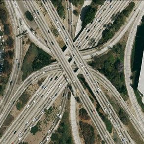
K. Nogueira et al.: Introduction to DeepMorphNets

designs, the pointwise convolutions exploited in the morpho-      1) IMAGE CLASSIFICATION DATASETS
logical layers have always the same configuration: kernel         a: SYNTHETIC DATASETS
1 × 1, stride 1, and no padding. Furthermore, all networks        As introduced, two simple synthetic (image classification)
receive input images with 224×224 pixels, use cross-entropy       datasets were designed in this work to validate the feature
as loss function, and SGD as optimization algorithm [1].          learning process of the proposed DeepMorphNets. In order
For the pixel classification task, the proposed networks were     to allow such validation, these datasets were created so that
exploited based on the pixelwise paradigm defined by [31],        it is possible to define, a priori, the optimal SE (i.e., the SE
in which each pixel is classified independently through a         that would produce the best results) for a classification sce-
context window.                                                   nario. Hence, in this case, the validation would be performed
   The first network is the simplest one, having just a unique    by comparing the learned SE with the optimal one, i.e., if
layer composed of one morphological opening M γ . This            both SEs are similar, then the proposed technique is able to
architecture was designed to be used with the proposed            perform well the feature learning step.
synthetic datasets (presented in Section IV-A1). Because              Specifically, both datasets are composed of 1,000
of this, it is referenced hereafter as DeepMorphSynNet.           grayscale images with a resolution of 224 × 224 pixels
Note that this network was only conceived to validate the         (a common image size employed in famous architecture such
learning process of the proposed framework as explained in        as AlexNet [2]) equally divided into two classes.
Section V-A.                                                          The first dataset has two classes. The first one is com-
   To analyze the effectiveness of the technique in a more        posed of images with small (5 × 5 pixels) squares whereas
complex scenario, we proposed a larger network inspired           the second consists of images with large (9×9 pixels) squares.
by the famous AlexNet [2] architecture. It is important to        Each image of this dataset has only one square (of one of the
highlight that AlexNet [2] was our inspiration, and not a more    above classes) positioned randomly. In this case, an opening
complex architecture, because if its simplicity, which allows     with a SE larger than 5 × 5 but smaller than 9 × 9 should
a clear analysis of the benefits of the proposed technique,       erode the small squares while keeping the others, allowing
thus avoiding confusing them with other advantages of more        the model to perfectly classify the dataset.
complex deep learning approaches. This proposed morpho-               More difficult, the second synthetic dataset has two
logical version of the AlexNet [2], called DeepMorphNet           classes of rectangles. The first class has shapes of 7 × 3
and presented in Figure 4, has the same number of layers          pixels while the other one is composed of rectangles of 3 × 7.
of the original architecture but fewer neurons in each layer.     As in the previous dataset, each image of this dataset has
Specifically, this network has 5 morphological and 3 fully        only one rectangle (of one of the above classes) positioned
connected layers, responsible to learn high-level features        randomly. This case is a little more complicated because the
and perform the final classification. To further evaluated the    network should learn a SE based on the orientation of one
potential of the proposed technique, in some experiments,         the rectangles. Particularly, it is possible to perfectly classify
a new version of the DeepMorphNet, using a modern com-            this dataset using a single opening operation with one of the
ponent called Selective Kernels (SK) [32], was developed          following types of SEs: (i) a rectangle of at least 7 pixels of
and experimented. This new network, referenced hereafter          width and height larger than 3 but smaller than 7 pixels, which
as DeepMorphNet-SK, uses such components to weigh the             would erode the first class of rectangles and preserve the sec-
features maps, giving more attention to some maps than the        ond one, or (ii) a rectangle with a width larger than 3 but
others.                                                           smaller than 7 pixels and height larger than 7 pixels, which
                                                                  would erode the second class of rectangle while keeping the
IV. EXPERIMENTAL SETUP                                            first one.
In this section, we present the experimental setup.
                                                                  b: UCMERCED LAND-USE DATASET
Section IV-A presents the datasets. Baselines are described
                                                                  This publicly available dataset [33] is composed of
in Section IV-B while the protocol is introduced
                                                                  2,100 aerial images, each one with 256 × 256 pixels and
in Section IV-C.
                                                                  0.3-meter resolution per pixel. These images, obtained from
                                                                  different US locations, were classified into 21 classes: agri-
A. DATASETS                                                       cultural, airplane, baseball diamond, beach, buildings, cha-
Six datasets were employed to validate the proposed Deep-         parral, dense residential, forest, freeway, golf course, harbor,
MorphNets. Two image classification synthetic ones were           intersection, medium density residential, mobile home park,
exclusively designed to check the feature learning of the         overpass, parking lot, river, runway, sparse residential, stor-
proposed technique. Other two image classification datasets       age tanks, and tennis courts. As can be noticed, this dataset
were selected to further verify the potential of DeepMor-         has highly overlapping classes such as the dense, medium,
phNets. Finally, to assess the performance of the pro-            and sparse residential classes which mainly differs in the
posed technique in distinct scenarios, two pixel classification   density of structures. Samples of these and other classes are
datasets were exploited.                                          shown in Figure 5.

114316                                                                                                                     VOLUME 9, 2021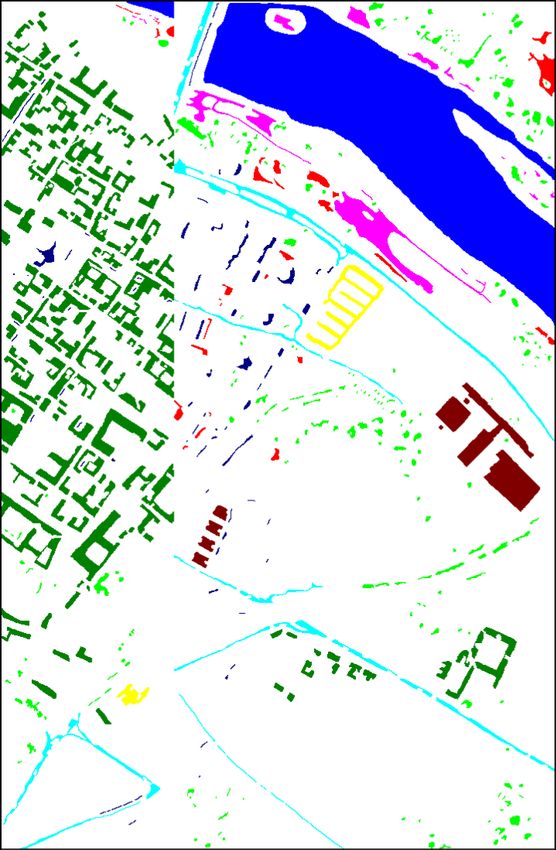
K. Nogueira et al.: Introduction to DeepMorphNets

FIGURE 4. The proposed morphological network DeepMorphNet conceived inspired by the AlexNet [2]. Since each layer is composed of distinct types of
morphological neurons, the number of each type of neuron in each layer is presented as an integer times the symbol that represents that neuron (as
presented in Section III-B). Hence, the total number of processing units in a layer is the sum of all neurons independently of the type. Also, observe that
the two depthwise convolutions of a same layer share the kernel size, differing only in the stride and padding. These both parameters are presented as
follows: the value related to the first depthwise convolution is reported separated by a comma of the value related to the second depthwise convolution.
Although not visually represented, the pointwise convolutions explored in the morphological layers always use the same configuration: kernel 1 × 1,
stride 1, and no padding.

FIGURE 5. Examples of the UCMerced Land-Use dataset.                            FIGURE 6. Examples of the WHU-RS19 dataset.

c: WHU-RS19 DATASET                                                              b: PAVIA UNIVERSITY
This public dataset [34] contains 1,005 high-resolution                         This public dataset [35] was also acquired by the ROSIS sen-
images with 600×600 pixels divided into 19 classes (approxi-                    sor during a flight campaign over Pavia. This hyperspectral
mately 50 images per class), including: airport, beach, bridge,                 image has 610 × 340 pixels, spatial resolution of 1.3m per
river, forest, meadow, pond, parking, port, viaduct, residential                pixel, and 103 spectral bands. Pixels of this image are also
area, industrial area, commercial area, desert, farmland, foot-                 categorized into 9 classes. The false-color and ground-truth
ball field, mountain, park and railway station. Exported from                   images, as well as the number of pixels in each class, are
Google Earth, that provides high-resolution satellite images                    presented in Figure 7.
up to half a meter, this dataset has samples collected from                        For both datasets, in order to reduce the computational
different regions all around the world, which increases its                     complexity, Principal Component Analysis (PCA) [36] was
diversity but creates challenges due to the changes in reso-                    used as a pre-processing method to reduce the dimension-
lution, scale, and orientation of the images. Figure 6 presents                 ality. Specifically, following [37], [38], for both datasets,
examples of some classes.                                                       we selected the first 3 principal components, which explain,
                                                                                approximately, 99% of the total variance of the data.
2) PIXEL CLASSIFICATION DATASETS
a: PAVIA CENTRE                                                                  B. BASELINES
This publicly available dataset [35] is composed of one                         Several baselines were employed in this work. The first one,
image, acquired by the Reflective Optics System Imaging                         exploited in both tasks and all aforementioned datasets, is a
Spectrometer (ROSIS), covering the city of Pavia, southern                      standard convolutional version of the corresponding Deep-
Italy. This hyperspectral image has 715×1.096 pixels, spatial                   MorphNet. This baseline, referenced as ConvNet, recreates
resolution of 1.3m per pixel, and 102 spectral bands. Pixels                    the exact morphological architecture using the traditional
of this image are categorized into 9 classes. The false-color                   convolutional layer but preserving all remaining configura-
and ground-truth images, as well as the number of pixels in                     tions (such as filter sizes, padding, stride, etc). Moreover,
each class, are presented in Figure 7.                                          this baseline makes use of max-pooling layers between the

VOLUME 9, 2021                                                                                                                                     114317
K. Nogueira et al.: Introduction to DeepMorphNets
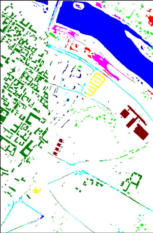
FIGURE 7. In the first (top) part, false-color and ground-truth images of the explored hyperspectral datasets. In the second (bottom) part,
the classes, the number of pixels used for training the models, and the total amount of labeled pixels.
convolutions, which makes it very similar to the traditional have the exact same number of layers and feature maps of
architectures of the literature [2]. An extension of this first the base DeepMorphNet. We believe that this conservation
baseline, referenced as PreMorph-ConvNet and exploited allows a fair comparison between the models given that
only for the (non-synthetic) image classification datasets, the potential representation of the networks is somehow the
uses pre-defined morphological operations as pre-processing same.
to extract the first set of discriminative features [20], [28].
Such data is then used as input to a ConvNet (in this case, C. EXPERIMENTAL PROTOCOL
the previously described one), which is responsible for per- For the synthetic datasets, a train/validation/test protocol was
forming the final classification. The third baseline, used employed. In this case, 60% of the instances were used
only for the (non-synthetic) image classification datasets and as training, 20% as validation, and another 20% as test.
referenced hereafter Depth-ConvNet, is exactly the Deep- Results of this protocol are reported in terms of the average
MorphNet architecture but without using binary weights accuracy of the test set. For the other image classification
and depthwise pooling. This baseline reproduces the same datasets, five-fold cross-validation was conducted to assess
DeepMorphNet architecture (also using depthwise and point- the accuracy of the proposed algorithm. The final results are
wise convolutions) and, consequently, has the same number the mean of the average accuracy (for the test set) of the
of parameters, except for the binary weights. Other base- five runs followed by its corresponding standard deviation.
lines, used only for the (non-synthetic) image classification Finally, for the pixel classification datasets, following pre-
datasets, are the deep morphological frameworks proposed vious works [38]–[40], we performed a random sampling to
by [23], [24]. In these cases, the DeepMorphNet architecture select 1,000 training samples/pixels from all classes, as pre-
was recreated using both techniques. Finally, the last base- sented in (the bottom part of) Figure 7. All remaining pixels
line, referenced with the suffix ‘‘SK’’ and explored only for are used to assess the tested architectures. The final results are
the (non-synthetic) image classification datasets, is the con- reported in terms of the average accuracy of those remaining
volutional and morphological networks, but with Selective pixels.
Kernels (SK) [32], which allows the network to give more All networks proposed in this work were implemented
importance to certain feature maps than to others. using PyTorch. All experiments were performed on a 64 bit
Differently from the morphological networks, all baselines Intel i7 5930K machine with 3.5GHz of clock, Ubuntu
use batch normalization [1] (after each convolution) and Rec- 18.04.1 LTS, 64GB of RAM memory, and a GeForce GTX
tified Linear Units (ReLUs) [30] as activation functions. It is Titan X Pascal with 12GB of memory under a 10.0 CUDA
important to note that, despite the differences, all baselines version.
114318 VOLUME 9, 2021You can also read