Agricultural Systems Contents lists available at ScienceDirect - CIMMYT Publications Repository
←
→
Page content transcription
If your browser does not render page correctly, please read the page content below
Agricultural Systems 198 (2022) 103383
Contents lists available at ScienceDirect
Agricultural Systems
journal homepage: www.elsevier.com/locate/agsy
Revisiting yield gaps and the scope for sustainable intensification for
irrigated lowland rice in Southeast Asia
João Vasco Silva a, b, *, Valerien O. Pede c, Ando M. Radanielson c, e, Wataru Kodama c,
Ary Duarte c, d, Annalyn H. de Guia c, Arelene Julia B. Malabayabas c, Arlyna Budi Pustika f,
Nuning Argosubekti f, Duangporn Vithoonjit g, Pham Thi Minh Hieu h, Anny Ruth P. Pame c,
Grant R. Singleton c, Alexander M. Stuart c
a
International Maize and Wheat Improvement Center (CIMMYT), Harare, Zimbabwe
b
Plant Production Systems, Wageningen University, Wageningen, the Netherlands
c
International Rice Research Institute (IRRI), Los Baños, Philippines
d
Universidade Federal de Santa Maria, Santa Maria, Brazil
e
University of Southern Queensland, Centre for Sustainable Agricultural Systems, Toowoomba, Australia
f
Indonesian Agency for Agricultural Research and Development, Jakarta Selatan, Indonesia
g
Chainat Rice Research Center, Chainat Province, Thailand
h
Department of Agriculture and Rural Development of Can Tho, Can Tho City, Viet Nam
H I G H L I G H T S G R A P H I C A L A B S T R A C T
• Analysis rice yield gaps is needed to
better understand how to sustainably
increase rice production across South
east Asia.
• Rice yield gaps (Yg) for four countries in
Southeast Asia were decomposed into
efficiency, resource, and technology
Ygs.
• Ygs were mainly attributed to resource
and technology Yg in Myanmar, and to
efficiency and technology Yg in
Indonesia.
• Yg closure requires increased N in
Myanmar, reduced N in Indonesia, and
fine-tuning N management in Thailand
and Vietnam.
• This novel approach identified oppor
tunities for sustainable intensification of
rice production in Southeast Asia.
A R T I C L E I N F O A B S T R A C T
Editor: Dr Jagadish Timsina CONTEXT: Recent studies on yield gap analysis for rice in Southeast Asia revealed different levels of intensifi
cation across the main ‘rice bowls’ in the region. Identifying the key crop management and biophysical drivers of
Keywords: rice yield gaps across different ‘rice bowls’ provides opportunities for comparative analyses, which are crucial to
Crop modelling better understand the scope to narrow yield gaps and increase resource-use efficiencies across the region.
Stochastic frontier analysis
* Corresponding author at: International Maize and Wheat Improvement Centre (CIMMYT-Zimbabwe), Zimbabwe.
E-mail addresses: j.silva@cgiar.org, joao.silva@wur.nl (J.V. Silva).
https://doi.org/10.1016/j.agsy.2022.103383
Received 18 August 2021; Received in revised form 28 January 2022; Accepted 1 February 2022
Available online 19 February 2022
0308-521X/© 2022 The Authors. Published by Elsevier Ltd. This is an open access article under the CC BY license (http://creativecommons.org/licenses/by/4.0/).
J.V. Silva et al. Agricultural Systems 198 (2022) 103383
Food security
OBJECTIVE: The objective of this study was to decompose rice yield gaps into their efficiency, resource, and
Smallholder agriculture
technology components and to map the scope to sustainably increase rice production across four lowland irri
gated rice areas in Southeast Asia through improved crop management.
METHODS: A novel framework for yield gap decomposition accounting for the main genotype, management, and
environmental factors explaining crop yield in intensive rice irrigated systems was developed. A combination of
crop simulation modelling at field-level and stochastic frontier analysis was applied to household survey data to
identify the drivers of yield variability and to disentangle efficiency, resource, and technology yield gaps,
including decomposing the latter into its sowing date and genotype components.
RESULTS AND CONCLUSION: The yield gap was greatest in Bago, Myanmar (75% of Yp), intermediate in
Yogyakarta, Indonesia (57% of Yp) and in Nakhon Sawan, Thailand (47% of Yp), and lowest in Can Tho, Vietnam
(44% of Yp). The yield gap in Myanmar was largely attributed to the resource yield gap, reflecting a large scope
to sustainably intensify rice production through increases in fertilizer use and proper weed control (i.e., more
output with more inputs). In Vietnam, the yield gap was mostly attributed to the technology yield gap and to
resource and efficiency yield gaps in the dry season and wet season, respectively. Yet, sustainability aspects
associated with inefficient use of fertilizer and low profitability from high input levels should also be considered
alongside precision agriculture technologies for site-specific management (i.e., more output with the same or less
inputs). The same is true in Thailand, where the yield gap was equally explained by the technology, resource, and
efficiency yield gaps. The yield gap in Indonesia was mostly attributed to efficiency and technology yield gaps
and yield response curves to N based on farmer field data in this site suggest it is possible to reduce its use while
increasing rice yield (i.e., more output with less inputs).
SIGNIFICANCE: This study provides a novel approach to decomposing rice yield gaps in Southeast Asia's main
rice producing areas. By breaking down the yield gap into different components, context-specific opportunities to
narrow yield gaps were identified to target sustainable intensification of rice production in the region.
1. Introduction area located in the Ayeyarwady delta (Thwe et al., 2019). Here, rice
productivity is significantly lower than in neighboring countries mostly
Rice (Oryza sativa L.) is the main staple food for more than half of the due to low input use, limited training, and poor infrastructure. However,
world's population, many of whom live in developing countries (Pandey the government recently set targets to double agricultural productivity
et al., 2010). Meeting the global rice demand in the future must be and farmers' incomes in a little over 10 years (Dubois et al., 2019).
achieved through sustainable increases in rice production in the main Strategies to increase food production and meet the future food de
rice growing areas of Southeast Asia to avoid further conversion of land mand must reconcile environmental and socio-economic factors with
to agriculture and to reduce the environmental and health impacts of narrowing (or maintaining) the existing yield gap between the potential
intensive production (Godfray et al., 2010; McKenzie and Williams, yield (Yp) for irrigated crops and the actual yield (Ya) observed in
2015). Other grand challenges facing agricultural systems worldwide farmers' fields (van Ittersum et al., 2013). Yield gap analysis plays a key
include the adverse effects of climate change, urban and industrial role in sustainable intensification research as it identifies the contribu
encroachment, biodiversity loss and associated loss of ecosystem ser tion of biophysical and management factors, and their interactions, to
vices and soil degradation (Silva and Giller, 2021; Bouman et al., 2007; actual yields (van Ittersum and Rabbinge, 1997; Evans and Fischer,
Rosegrant and Cai, 2002). Against this background, sustainable inten 1999; van Ittersum et al., 2013). Yet, to increase crop yields sustainably,
sification was proposed as a strategy to increase crop productivity, it is also important to understand the broader socio-economic context in
through yield gap closure on existing agricultural land, while improving which farmers operate to prioritize the ‘sustainability’ and ‘intensifica
resource-use efficiencies and reducing environmental externalities tion’ pathways most suitable for a given farming system (Laborte et al.,
(Cassman and Grassini, 2020; Tilman et al., 2011). 2012; Stuart et al., 2016; Struik and Kuyper, 2017; Silva et al., 2021).
Assessing the potential for sustainable intensification is particularly Comparative studies, building upon common frameworks and methods,
important in many Asian countries where rice is the staple food and of farming systems in different stages of intensification or affected by
irrigated lowland rice occupies a large proportion of the total agricul different structural transformation of national economies are particu
tural land (GRiSP, 2013). Indonesia, Vietnam, Thailand, and Myanmar larly useful in this regard.
are responsible for nearly 85% of the annual rice production in South Recent studies on yield gap analysis for rice in Southeast Asia
east Asia (FAOSTAT, n.d.). Indonesia is the 3rd world's largest rice revealed different levels of intensification across the main ‘rice bowls’ in
producer and has been able to achieve near self-sufficiency in recent the region (e.g., Laborte et al., 2012; Stuart et al., 2016; Silva et al.,
years (Agus et al., 2019). However, some of the country's most pro 2017a, 2017b; Radanielson et al., 2019). Such diversity provides op
ductive agricultural areas, such as in Java, are being lost as land is portunities for identifying the key biophysical and management drivers
converted to residential, commercial, or other purposes (Rumanti et al., of rice yield gaps in a comparative way and, hence, to explore oppor
2018). Vietnam has become one of the world's largest rice exporters, and tunities to narrow yield gaps and increase resource-use efficiencies. This
the Mekong delta produces nearly 60% of Vietnam's total rice output study revisits the analysis of Stuart et al. (2016) and expands it with a
(Tong, 2017). However, the rapid intensification of rice production in field-specific yield gap decomposition for two growing seasons, repre
Southern Vietnam from the late 1990s resulted in an overreliance on senting one annual cropping cycle, across four main irrigated lowland
agrochemicals that are becoming increasingly expensive (Stuart et al., rice areas in Southeast Asia. By doing so, best-bet crop management
2018a), which makes it important to consider improvements in practices and pathways for sustainable intensification attuned to local
resource-use efficiency and profitability in addition to increases in rice conditions can be identified and used to inform policy. The objective of
yield. The same is true in Thailand, one of the world's largest rice pro the present study was two-fold: 1) to decompose rice yield gaps while
ducers and exporters. About half of the total annual rice produced in identifying the key biophysical and management constraints to rice
Thailand comes from the Chao Phraya river basin (Stuart et al., 2018b), yield, and 2) to explore pathways for sustainable intensification across
where rising rural wages and input costs have magnified the focus on four irrigated lowland rice areas in Southeast Asia in a comparative way.
increasing the profitability of rice production. Lastly, Myanmar is the To do so, crop growth modelling was applied to simulate Yp under
fourth largest rice producer in Southeast Asia, with over 55% of the rice different management scenarios and stochastic frontier analysis was
2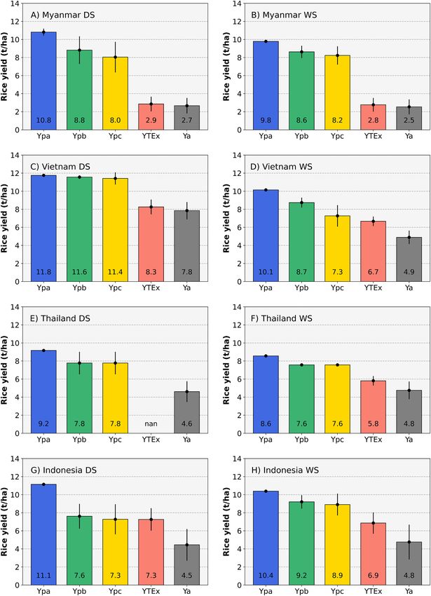
J.V. Silva et al. Agricultural Systems 198 (2022) 103383
used to decompose yield gaps across a sample of rice fields in each of the of inputs in a well-defined biophysical environment (Silva et al., 2017a,
irrigated lowland sites studied. 2017b). YTEx can be estimated with methods of frontier analysis (Farrell,
1957) applied to individual farmer field data containing detailed in
2. Concepts and definitions formation on crop yield, input use, management practices, and bio
physical conditions. Second, the actual yield (Ya) refers to the yield
Yield potential (Yp) is defined as the yield of a crop cultivar in a observed in farmers' fields as requested in e.g., farm surveys.
given cropping season when grown with water and nutrients non- Four major yield gaps can be estimated based on the five yield levels
limiting and biotic stresses effectively controlled (Evans, 1993; van previously introduced (Fig. 1). The total yield gap refers to the differ
Ittersum and Rabbinge, 1997). Three variants of Yp are defined in this ence between Ypa and Ya, which can also be expressed by the ratio
study to consider the impact of the main factors controlled by farmers between Ya and Ypa defined as yield gap closure. The total yield gap can
driving Yp variability namely sowing dates and variety characteristics be further decomposed into technology, resource, and efficiency yield
(Fig. 1). gaps (see Silva et al., 2017a, 2017b) for a visual illustration of these
Ypa refers to the potential yield simulated with a crop growth model concepts).
for the highest yielding variety and for the optimum sowing date of the The technology yield gap is quantified here as the difference between
cropping season within a given site. Ypa is thus an indicator of the po Ypa and Ypc, which indicates the yield gap due to sub-optimal sowing
tential yield of a given site for a given season using the optimum sowing date and variety choice from a production perspective. The use of Ypc in
date and the highest yielding variety available to farmers. The optimum the calculation of the technology yield gap, instead of the highest
sowing date of the growing season was defined as the date with the farmers' yields (YHF, i.e., the average Ya for the fields above the 90th
highest Yp within a three-month sowing window around the mean percentile of Ya) as in Silva et al. (2017a, 2017b), implies that the
sowing date observed in farmer's field data for a particular season (i.e., technology yield gap estimated here is only explained by sowing prac
mean sowing date ± 6 weeks). tices and crop varieties differing between Ypa and Ypc. When the tech
Ypb refers to the potential yield simulated with a crop growth model nology yield gap is defined as the difference between Ypa and YHF, as in
for the highest yielding variety and for the field-specific sowing dates Silva et al. (2017a, 2017b), then its magnitude can be attributed to
observed in a given site. The highest yielding variety used as a bench resource yield gaps of specific inputs (i.e., partial shifts of the production
mark for Ypa and Ypb was the variety with the highest average Yp, frontier) or to the adoption of precision agriculture practices, new va
among the varieties used by farmers, in a given growing season. Ypb rieties, or manipulation of sowing practices (i.e., total shifts of the
informs about the potential yield for the sowing date reported in an production frontier; Silva et al., 2017a, 2017b). Conversely, when the
individual field and considering the highest yielding variety available. technology yield gap is defined as the difference between Ypa and Ypc, as
Ypa and Ypb are then indicators of yield potential for the highest yielding done in this study, then it can only be attributed to the latter factors. In
variety available at each site when it is grown in the optimum sowing this way, the technology yield gap can be further disaggregated into a
date and in the farmer reported sowing date, respectively. ‘sowing date yield gap’ (the difference between Ypa and Ypb) and a
Ypc refers to the potential yield simulated with a crop growth model ‘genetic yield gap’ (the difference between Ypb and Ypc; Fig. 1). The
considering both varieties and sowing dates as observed in farmers' sowing date yield gap is explained by sub-optimal sowing dates and
fields. Thus, Ypc refers to the actual variety used by the farmer on its hence, considers yield response to environmental conditions during the
actual sowing date. As defined here, the difference between Ypb and Ypc growing season (Jing et al., 2008; Rattalino Edreira et al., 2017; Rada
does not consider genotype x sowing date interactions, which are known nielson et al., 2019). The genetic yield gap is attributed to lower per
to influence resource use efficiencies at crop (Evans and Fischer, 1999) forming varieties from a production perspective as also introduced by
and cropping systems levels (Guilpart et al., 2017). Ypb and Ypc consider Senapati and Semenov (2020).
observed sowing dates and the results must be interpreted accordingly, The resource yield gap is quantified here as the difference between
as explained by the variety used. Ypc and YTEx, hence it indicates the yield gap associated with insufficient
Two additional yield levels are defined to capture crop productivity amounts of inputs applied in farmers' fields, which limits the capacity to
under actual farm conditions (Fig. 1). First, the technical efficient yield achieve Ypc. The use of Ypc to estimate the resource yield gap is com
(YTEx) refers to the highest possible yield obtained given observed levels parable to the concept of ‘feasible yield’ (Yf; van Dijk et al., 2017) and to
Fig. 1. Concepts and definitions of the yield levels and
yield gaps used in this study for decomposing rice yield
gaps across irrigated lowland areas in Southeast Asia.
Abbreviations: Ypa, simulated potential yield for optimum
sowing date and the highest yielding variety; Ypb, simu
lated potential yield for farmers' sowing dates and highest
yielding variety; Ypc, simulated potential yield for
farmers' sowing dates and variety used; YTEx, technical
efficient yield estimated with stochastic frontier analysis;
Ya, actual yield observed in farmers' fields. Please refer to
Section 2 for further information about these yield levels.
3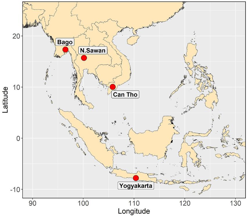
J.V. Silva et al. Agricultural Systems 198 (2022) 103383
the concept of ‘highest-farmers' yield’ (YHF) in high-yielding cropping interviewed in Bago (2012), Can Tho (2015), Yogyakarta (2014), and
systems (Silva et al., 2017a, 2017b). Yet, Ypc assumes optimal resource- Nakhon Sawan (2013), respectively. A subset of the data from the same
use efficiencies from an agronomic perspective, whereas Yf and YHF survey were reported by Stuart et al. (2016; for the wet season only) and
consider the maximum resource-use efficiencies realized in farmers' Devkota et al. (2019). Additional data on the socio-economic charac
fields. teristics, rice variety duration, sowing window, and herbicide use are
Finally, the efficiency yield gap is quantified as the difference be included in this study.
tween YTEx and Ya and hence captures the contribution of different The actual yield (adjusted to 14% moisture content) was calculated
techniques in the use of the technology and resources to actual yields, as the ratio between actual rice production and field area. Individual
translating into sub-optimal time, space, and form of the inputs applied. cases where Ya was greater than Ypc plus 0.5 t ha− 1 were removed from
Crop management in relation to a) ‘time’ refers to the timing of appli the analysis (i.e., Myanmar, n = 0; Vietnam, n = 5; Thailand, n = 1;
cation of the different inputs used by farmers, b) ‘space’ refers to the Indonesia, n = 21, where n stands for the number of observations
spatial variability of input requirement and application, the variability excluded from the analysis in each site). Possible reasons for these
in soil types and their effects on input use efficiency and, c) ‘form’ refers extreme values are: 1) misidentification of the rice variety sown, 2)
to the type of inputs used by farmers. underestimation of field size, and/or 3) overestimation of actual rice
production. Descriptive statistics of selected agronomic and socioeco
3. Materials and methods nomic factors in each site are presented in Table 1.
Bago, Myanmar, has two major growing seasons per year: the sum
3.1. Study area and household surveys mer season or dry season (DS) from November to May and the monsoon
season or wet season (WS) from June to January. In Can Tho, Vietnam,
The study area includes four sites in irrigated lowland rice areas of double rice cropping is also dominant, with a winter-spring or DS crop
Southeast Asia (Fig. 2), namely Bago (Ayeyarwady delta, Myanmar), from November to March and a summer-autumn or WS crop from April
Can Tho (Mekong delta, Vietnam), Nakhon Sawan (Chao Phraya river to July. Farmers in Nakhon Sawan, Thailand, typically grow two rice
basin, Central Thailand) and Yogyakarta (Java, Indonesia). In each site, crops per year: a DS crop from January to May and a WS crop from June
four different administrative units (village or commune) were purposely to October. In Yogyakarta, Indonesia, rice is grown up to three times a
selected as possible intervention sites for the Closing Rice Yield Gaps in year in some areas: a WS crop from November to March, an early DS
Asia with Reduced Environmental Footprint (CORIGAP) project. Each of crop from April to July, and a late DS crop from July to October. Farmers
the sites represents irrigated lowland rice production, with at least two that do not have sufficient water to grow a second DS crop, typically
rice crops grown each year. Within each country, villages were selected grow a non-rice dryland crop (i.e., “palawija”, such as maize, mung bean,
based on similar farm size and demographic characteristics and were or groundnut).
located within a 25 km radius of each other. In Bago, Can Tho and
Yogyakarta, survey respondents were randomly selected from a list of 3.2. Crop model simulations to estimate the potential yield (Yp)
rice farmers from each administrative unit, whereas in Nakhon Sawan,
interviews were conducted with all the farmers from a community rice The crop model ORYZA v3 (Li et al., 2017) was used to simulate the
center within each administrative unit. The farm surveys were con three variants of Yp considered in this study (Fig. 1). These Yp variants
ducted between 2012 and 2015, depending on the site. Farmers were were simulated for each surveyed field in each site where the farm
interviewed using a standard structured questionnaire across all sites surveys were conducted. The ORYZA v3 model, and its earlier versions,
requesting information for the largest rice parcel in each farm on inputs has been extensively calibrated and evaluated to simulate Yp for rice in
used, crop management practices, actual rice production, and field area the main irrigated rice areas of Southeast Asia (Jing et al., 2008; Laborte
for the previous two cropping seasons, as well as a set of farm and et al., 2012; Li et al., 2016; Stuart et al., 2016; Radanielson et al., 2019).
household characteristics. A total of 100, 180, 180 and 84 farms were The model represents rice crop development and growth in response to
genotypic, environmental and management factors, and their in
teractions, considering mechanistic and empirical relationships that are
described in Bouman et al. (2001) and Li et al. (2017).
The factors considered in the simulation of Yp included daily
weather data for each site where the farm surveys were conducted
(Table 1) as well as field-specific farmers' reported rice varieties, crop
establishment method and sowing dates (Table 2). For each farmers'
field surveyed, daily weather data were obtained from the NASA
POWER database (http://power.larc.nasa.gov). These data included
daily minimum and maximum temperatures, solar radiation, and rain
fall (Suppl. Fig. 1). The varieties simulated in each site were IR50 (Shwe
Thwe Yin), IR138 (Mestizo) and IR154 (NSIC Rc222) in Myanmar,
Jasmine 85 and OM5451 in Vietnam, RD31 in Thailand, and Ciherang,
IR64 and Inpari 6 in Indonesia (Table 2). The main differences between
these calibrated varieties in ORYZA v3 are the thermal times controlling
crop development and some of the parameters controlling leaf growth
and biomass production. Further details about the calibration of the
different varieties in ORYZA v3 are reported elsewhere (Boling et al.,
2004; Boling et al., 2010; Stuart et al., 2016; Radanielson et al., 2018;
Radanielson et al., 2019) and the calibrated crop files for each variety
can be found at https://github.com/andomariot/inputs_cropfile_oryza/f
ind/main. If the variety reported by the farmer was not identified among
the previously mentioned varieties, then the variety used in the crop
Fig. 2. Location of the irrigated lowland rice areas analyzed in this study: Bago model simulations was the most reported variety among the farmers
in Myanmar, Nakhon Sawan in Thailand, Can Tho in Vietnam, and Yogyakarta surveyed in Vietnam, Thailand, and Indonesia, respectively. This allows
in Indonesia. maintaining consistency in Ypc and reducing uncertainties in Yp
4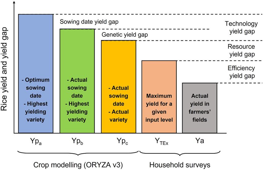
J.V. Silva et al. Agricultural Systems 198 (2022) 103383
Table 1
Descriptive statistics of selected agronomic and socioeconomic factors for dry season (DS) and wet season (WS) rice across four irrigated lowland areas in Southeast
Asia. Average values are shown for each variable with standard deviations between brackets.
Myanmar Vietnam Thailand Indonesia
DS WS DS WS DS WS DS WS
Actual yield (t ha− 1) 2.67 2.54 7.86 4.94 4.61 4.75 4.95 4.84
(0.86) (0.83) (0.96) (0.84) (1.14) (0.98) (2.17) (1.94)
Input use and management
N applied (kg N ha− 1) 30.27 17.53 102.48 92.89 83.86 82.04 197.03 211.77
(20.09) (18.72) (29.53) (31.90) (28.96) (36.42) (103.03) (117.33)
P applied (kg P ha− 1) 1.03 0.37 27.70 25.97 16.68 16.67 18.71 20.21
(2.55) (1.40) (10.32) (10.97) (8.82) (9.33) (11.89) (13.68)
K applied (kg K ha− 1) 0.14 0.00 42.80 39.23 9.55 9.39 36.25 38.44
(0.62) (0.01) (20.11) (19.40) (15.96) (14.87) (23.81) (24.96)
Fertilizer splits (#) 1.61 0.89 3.69 3.62 2.79 2.65 2.38 2.44
(0.87) (0.83) (0.82) (0.86) (0.41) (0.48) (0.76) (0.68)
Herbicide use (=1 if yes) 0.51 0.00 0.94 0.96 0.53 0.96 0.04 0.02
(0.50) (0.00) (0.24) (0.19) (0.50) (0.19) (0.20) (0.13)
Sowing week1 12.13 7.44 1.11 2.91 7.33 5.17 8.03 2.75
(17.19) (3.62) (0.94) (1.70) (14.42) (1.67) (2.92) (2.13)
Duration of rice varieties2
Short duration (=1 if yes) 0.04 0.00 0.11 0.63 0.00 0.00 0.21 0.18
(0.20) (0.00) (0.32) (0.48) (0.00) (0.00) (0.41) (0.38)
Medium-short duration (=1 if yes) 0.39 0.12 0.89 0.37 0.82 0.92 0.76 0.80
(0.49) (0.32) (0.32) (0.48) (0.39) (0.28) (0.43) (0.40)
Medium-long duration (=1 if yes) 0.46 0.49 0.00 0.00 0.00 0.00 0.00 0.00
(0.50) (0.50) (0.00) (0.00) (0.00) (0.00) (0.00) (0.00)
Long duration (=1 if yes) 0.14 0.38 0.00 0.00 0.18 0.08 0.00 0.00
(0.35) (0.49) (0.00) (0.00) (0.39) (0.28) (0.00) (0.00)
Socioeconomic characteristics
Farm experience (year) 25.07 25.56 25.25 25.33 23.29 25.70 23.42 22.84
(11.95) (11.91) (10.00) (10.04) (13.94) (14.16) (15.95) (15.01)
Ratio of rice income (%)3 53.92 40.93 46.63 9.44 37.11 32.67 49.59 24.47
(36.46) (35.18) (28.34) (11.17) (19.54) (24.17) (20.26) (20.59)
Farm size (ha) 3.03 4.87 2.16 2.14 4.43 4.84 0.17 0.18
(4.27) (5.38) (0.97) (1.00) (3.14) (3.39) (0.16) (0.18)
Observations 98 93 177 162 49 83 117 118
1
Sowing week refers to the number of weeks deviated from the optimum sowing date identified with crop modelling (cf. Table 2).
2
The category of rice variety is based on the duration of the growing season as follows. short = 95 days or less, medium-short = 96–120 days, medium-long =
121–140 days, and long = greater than 140 days.
3
Ratio of rice income (%) denotes the share of ’a’ rice income over annual farm income.
estimates associated with farmer's variety as the most used varieties are 3.3. Stochastic frontier analysis and estimation of technical efficient
known to be available for farmers in the respective site and are likely to yields (YTEx)
be used and representative of the variety used by a given farmer. In
Myanmar, none of the varieties previously calibrated in ORYZA v3 were Stochastic frontier analysis is a parametric method of frontier anal
used by the surveyed farmers, thus the calibrated variety with the most ysis that separates the effects of statistical noise and technical in
similar crop growth duration in relation to the variety reported by efficiency in the production process (Aigner et al., 1977; Meeusen and
farmers was used in the crop model simulations. The calibrated varieties Van Den Broeck, 1977). Stochastic frontier analysis was used to estimate
used in the simulations were IR50 for short-duration varieties, IR38 for the technical efficient yield (YTEx) and the efficiency yield gap (i.e.,
medium-duration varieties, and IR154 for long-duration varieties. difference between YTEx and Ya). The approach considers the effects of
Farmers reporting varieties with more than 130 days, that were not biophysical control variables and production factors on crop yields
defined with photoperiod sensitivity, were classified as long-duration while estimating two random errors, vi and ui. The former (vi) captures
varieties. Similarly to previous studies (e.g., van Oort et al., 2011; Li random shocks and noise in the response variable (i.e., crop yield),
et al., 2015), the calibration of a specific variety may increase un whereas the latter (ui) captures the contribution of sub-optimal crop
certainties in Ypc due to limited information from the farm survey on the management in relation to the time, space and form of the inputs used
characteristics of the variety and the inherent uncertainties in yield and (Silva et al., 2017a, 2017b). The two random errors are thus important
crop phenology reported. Furthermore, most varieties recommended at to isolate possible inaccuracies in the reported Ya from inefficient crop
the respective study sites were referred to by their growth duration class management practices. YTEx was estimated from a stochastic frontier
in addition to their name. model assuming a Cobb-Douglas functional form (i.e., considering first-
Over 95% of the surveyed farmers in Vietnam and Thailand used order terms only) and accounting for inefficiency effects as follows:
direct-seeding as their crop establishment method, whereas in Indonesia ∑K
all farmers used transplanting. Thus, in the aforementioned sites, the lnyi = α0 + β lnxki + vi − ui
k k
(1)
dominant crop establishment method reported in the farm survey was ( )
used in the crop model simulations (Table 2). Conversely, 53% and 90% vi ∼ i.i.d.N 0, σ2v (2)
of the farmers in Myanmar used transplanting in the DS and WS,
( ) ∑J
respectively, thus the crop establishment method reported by the ui ∼ i.i.d.N + μ, σ 2u , μ = δj zji (3)
farmers was used in the crop model simulations.
j
YTExi = Yai × exp ( − ui )− 1
(4)
5
J.V. Silva et al. Agricultural Systems 198 (2022) 103383
Table 2 duration ranging from 95 to 110 days was simulated using IR50. Yp for long
Input data and assumptions used in the ORYZA v3 crop model to simulate the duration varieties with more than 110 days was simulated using NSIC Rc222.
4
three variants of the potential yield (Yp) defined in this study (cf. Fig. 1) for the Boling et al. (2010).
5
farmer's fields surveyed across four lowland rice irrigated rice areas in Southeast Radanielson et al. (2019).
6
Asia. Stuart et al. (2016).
Input data Description
Myanmar where yi is the actual yield (t ha− 1) of farmer i, and xi is a vector of inputs
Farmer's sowing window 23-Nov-2011 to 11-Apr-2012 and agronomic practices used by farmer i. The error term vi is assumed to
DS be independently and identically distributed (i.i.d.) following a normal
Farmer's sowing window 07-Jun-2011 to 20-Sep-2011
WS
distribution with mean 0 and variance σ v2. The error term ui is also
Optimum sowing date 25-Jan-2012 assumed to be i.i.d. but with a truncated-normal distribution with mean
∑
DS1 μ = jJδjzji and variance σ u2,where zi represents a vector of agronomic
Optimum sowing date 14-Sep-2011 and socioeconomic variables explaining the efficiency yield gap. β and δ
WS1
are season-specific parameters to be estimated with maximum likeli
Crop establishment2 Transplanting and direct seeding
Varieties calibrated in Shwe Thwe Yin5 (IR50; 105–110 days), Mestizo5 (IR 138; hood as described in Wang and Schmidt (2002). A log-likelihood ratio
Oryza3 90–95 days), test was used to determine the appropriate specification between a
RC2223 (IR154; 105–110 days) Cobb-Douglas (Eq. (1)) and a specification for the production frontier
RC2225 (IR 154; 105–110 days) including interactions between the continuous variables. The result of
If not calibrated 100 < 130 days = Mestizo; >130
the log-likelihood ratio test indicated that a Cobb-Douglas functional
days = RC222
Highest yielding variety RC222 form was more appropriate than the specification with interaction terms
for both seasons in Myanmar and Indonesia (data not shown). Thus, the
Vietnam
Farmer's sowing window 22-Oct-2014 to 24-Dec-2014
parameter estimates of the Cobb-Douglas functional form are presented
DS in the main manuscript (Table 3) and the parameter estimates of the
Farmer's sowing window 05-Mar-2014 to 24-May-2014 specification with interaction terms are presented in Suppl. Table S2.
WS The parameters of the production function (Eq. (1)) and the inefficiency
Optimum sowing date 26-Nov-2014
effects (Eq. (3)) were estimated simultaneously with the sfcross() func
DS1
Optimum sowing date 5-Mar-2014 tion from the Stata package sfcross (Belotti et al., 2013) and with the
WS1 dependent and independent variables log-transformed. YTEx was calcu
Crop establishment Direct seeding lated based on the error term ui following Eq. (4).
Varieties calibrated in Jasmine 856 (100–105 days), OM54516 (90–95 days)
The stochastic frontier models were fitted for each site x season
Oryza
If not calibrated Jasmine 85 (most sown)
combination. The only exception was the DS data in Thailand for which
Highest yielding variety Jasmine 85 the small sample size did not allow for reliable estimation of the pro
duction frontier. The vector of inputs xi included six variables defined
Thailand
Farmer's sowing window 24-Oct 2012 to 23-Jan-2013 according to principles of production ecology (van Ittersum and Rab
DS binge, 1997). The variables referring to growth-defining factors
Farmer's sowing window 15-May-2013 to 14-Aug-2013 included in the model were the sowing date (defined as the deviation
WS expressed in number of weeks from the optimum sowing date identified
Optimum sowing date 20-Dec-2012
DS1
with the crop model simulations) and type of rice variety grown (short-,
Optimum sowing date 29-May-2013 medium-, and long-duration varieties, considering the latter as the
WS1 reference category). The amounts of nitrogen (N), phosphorus (P) and
Crop establishment Direct seeding potassium (K) applied were included in the model to capture the effects
Varieties calibrated in RD316 (120–125 days)
of growth-limiting factors on crop yields. Herbicide use (yes or no) was
Oryza
If not calibrated RD31 the only variable included in the model to capture the effects of growth-
Highest yielding variety RD31 reducing factors on crop yields. Variables capturing the management of
pests and diseases, or their incidence, in the surveyed fields, were not
Indonesia
Farmer's sowing window 06-Mar-2013 to 14-Aug-2013 considered due to lack of data. The effects of climatic conditions on rice
DS yields were assumed to be partly captured by the sowing date variable
Farmer's sowing window 02-Oct-2013 to 25-Dec-2013 and no other control variables for variation in soil types were included in
WS
the analysis given the flat topography of the sites and the proximity of
Optimum sowing date 5-Jun-2013
DS1 the fields surveyed (see Section 3.1).
Optimum sowing date 18-Dec-2013 The variability in the efficiency yield gap was explained using a
WS1 second-stage regression in the production frontier (Eq. (3)). The drivers
Crop establishment Transplanting of the efficiency yield gap, zi, included in the analysis were the number
Varieties calibrated in Ciherang6 (115–120 days), IR644 (95–100 days) and
of fertilizer splits (#), the years of farming experience of the household
Oryza Inpari 6 (120–125 days)
If not calibrated Ciherang (most sown) head (# years), and the share of rice income in a given season to total
Highest yielding variety Inpari 6 annual income (%, see Section 3.4 for a definition of total annual in
1 come). It is hypothesized that efficiency yield gaps decrease with in
The optimum sowing date was estimated on a three-month window around
the average actual sowing date, as the survey data showed a large range of creases in farming experience and increases in the share of rice income
sowing dates. to total annual income as such conditions may contribute to better crop
2
In Myanmar the crop establishment method was set individually for each management in terms of time, space, and form of the inputs applied. A
farmer. positive sign on an estimated coefficient in the production frontier (Eq.
3
In Myanmar there was a wide range of varieties sown by the farmers, and (1)) indicates a productivity increasing factor, while a negative coeffi
none of them was calibrated in ORYZA v3, so the actual varieties were classified cient in the inefficiency estimation (Eq. (3)) indicates a reduction of the
according to their duration. Yp for varieties with growth duration lower than 95 efficiency yield gap.
days was simulated using the variety IR38. Yp for varieties with medium
6
J.V. Silva et al. Agricultural Systems 198 (2022) 103383
Table 3
Parameter estimates of the stochastic frontier models estimated for dry season (DS) and wet season (WS) rice across four lowland irrigated rice areas in Southeast Asia.
The effect of interactions between variables are presented in Supplementary Table S2.
Myanmar Vietnam Thailand Indonesia
DS WS DS WS WS DS WS
Production frontier
Nitrogen log 0.024 0.085*** 0.089** 0.377*** − 0.079 0.089*** 0.107*
(0.019) (0.014) (0.038) (0.087) (0.057) (0.030) (0.055)
Phosphorus log − 0.001 − 0.172*** − 0.016 0.011* 0.030
(0.022) (0.060) (0.021) (0.005) (0.028)
Potassium log 0.010 0.069*** 0.006
(0.014) (0.023) (0.009)
Herbicide use 0.294*** − 0.060* 0.254***
(0.056) (0.036) (0.066)
Sowing week 0.000 − 0.010 0.004 − 0.006 − 0.027*** 0.020 − 0.017
(0.002) (0.007) (0.010) (0.010) (0.010) (0.020) (0.015)
Short duration 0.008 0.173*** − 0.098 − 0.098
(0.027) (0.044) (0.196) (0.080)
Medium-short duration 0.043 0.062 − 0.047
(0.083) (0.082) (0.060)
Medium-long duration 0.012 0.029
(0.077) (0.054)
Constant 7.654*** 7.747*** 8.558*** 6.896*** 9.035*** 8.506*** 8.157***
(0.107) (0.082) (0.175) (0.273) (0.302) (0.345) (0.320)
Inefficiency term
Fertilizer splits − 0.106 0.205 0.361 1.092 − 65.752 0.089 0.030
(0.069) (0.223) (0.903) (0.784) (186.922) (0.091) (0.145)
Farm experience log 0.053 0.360 − 0.964 3.714*** − 0.706 − 0.054 0.072
(0.110) (0.394) (2.181) (0.815) (15.132) (0.078) (0.113)
Ratio of rice income 0.045 − 0.132 − 0.021 − 0.281 − 0.607 − 0.008** − 0.042***
(0.045) (0.095) (0.051) (0.534) (1.811) (0.003) (0.016)
Constant − 4.207 − 1.486 1.004 − 2.847 2.204 1.035*** 0.460
(4.590) (1.653) (1.902) (2.736) (3.816) (0.350) (0.512)
Model performance
TE score 0.929 0.912 0.947 0.707 0.821 0.495 0.692
σ 2 = σ u 2 + σ v2 0.360*** 0.588*** 0.447*** 0.781*** 4.833*** 0.516*** 0.727***
λ = σu2/σ2 0.313*** 0.626*** 0.770*** 0.810*** 0.987*** 0.999*** 0.697***
Observations 98 92 177 162 83 83 115
Significance is indicated by the following codes: * P < 0.10, ** P < 0.05, and *** P < 0.01; Parenthesis show standard error of estimated coefficients. Skewed variables
(i.e., mean < 0.05 or mean > 0.95 for binary variables), were not include in the analysis; Reference codes for variety types were as follows: Myanmar = long-duration,
Vietnam = medium-short duration, Thailand = long-duration, Indonesia = medium-short duration.
3.4. Statistical analysis yield loss associated with spikelet sterility (Suppl. Fig. 2). Indeed, rice
crops sown between mid-December and mid-January had on average a
Variability in farm size (ha) and share of rice income to total annual 25% lower Ypb than crops sown between late January and early
income (%) across sites was analyzed using boxplots. Total annual in February (Fig. 4A; Suppl. Fig. 2).
come is the sum of annual rice income and annual non-rice income, with During 2012 WS, the Ypa in Bago was on average 9.8 t ha− 1, Ya was
the latter including income from a salary earner at private firms with 2.5 t ha− 1 and the yield gap between Ypa and Ya was 7.3 t ha− 1 (Fig. 3B;
regular pay, a salary earner at public facilities, a casual wage earner, Suppl. Table S1). The yield gap was mainly attributed to the resource
wages from farm labor and, selling farm products other than rice. Rice yield gap (55% of Ypa) and to the technology yield gap (16% of Ypa;
yield response to N applied was assessed using quantile regression fitted Fig. 3B). The sowing window during the WS was narrower than during
to the 90th percentile of the pooled data with the smf() function of the the DS (between June and September), thereby lowering the contribu
statsmodels library in Python (Seabold and Perktold, 2010). A logistic tion of the sowing date yield gap to 12% of Ypa (Fig. 3B). The genetic
functional form (y = a + b × x + c × 0.99x) was assumed for this yield gap was small in both seasons accounting for less than 8% of Ypa
relationship, where y refers to actual yield (in t ha− 1) or yield gap (Fig. 3A and B). A total of 12 and 10 rice varieties were grown in the DS
closure (% of Ypa) and x refers to the total amount of N applied with and WS, respectively, with the most used varieties, Manaw Thukka and
mineral fertilizers in each field. Hmaw Be, sown by 41% and 35% of respondents, respectively (data not
shown).
4. Results The major driver for rice yield variability in Bago was the use of
herbicides in the DS and the amount of N applied in the WS (Table 3).
4.1. Bago, Ayeyarwady delta, Myanmar During the DS, fields where herbicides were used yielded ca. 30% more
than fields where no herbicides were used (Table 3). N applied had a
During 2012 DS, Ypa in Bago was on average 10.8 t ha− 1, Ya was 2.7 statistically significant positive effect on rice yield in the WS only, but
t ha− 1 and the respective yield gap between Ypa and Ya was 8.1 t ha− 1 the effect was small. Indeed, no clear yield response to N applied was
(Fig. 3A; Suppl. Table S1). The yield gap was mainly attributed to the observed within the sample for Myanmar (Fig. 5). The small effect of N
resource yield gap (47% of Ypa) and to the technology yield gap (25% of applied on rice yield in this site can be explained by the low N appli
Ypa; Fig. 3A). During the DS, the technology yield gap was mostly cation rates observed in all surveyed fields, which ranged between nil
explained by the sowing date yield gap (20% of Ypa, Fig. 3A). There was and 50 kg N ha− 1 in both seasons (Fig. 5), and possibly by other factors
a large sowing window (November to April; Fig. 4A) in the DS resulting associated with poor crop management. This range of N application rate
in a large variability of Ypb with risk of high temperature, leading to was the lowest observed across the four sites. Although there was no
7
J.V. Silva et al. Agricultural Systems 198 (2022) 103383
Fig. 3. Rice yields and yield gap decomposition into efficiency, resource, and technology yield gaps across four irrigated lowland rice areas in Southeast Asia. Values
in each bar indicate the average across all fields analyzed in each site. Abbreviations are as defined in Fig. 1.
statistically significant effect of the proportion of rice income to total 4.2. Can Tho, Mekong delta, Vietnam
farm income on the efficiency yield gap (Table 3), increasing rice pro
duction in Bago is likely to improve farm profitability because ca. 80% of During 2015 DS, the mean Ypa in Can Tho was 11.8 t ha− 1, Ya was
the total annual income was derived from rice farming alone and most 7.8 t ha− 1 and the respective yield gap between Ypa and Ya was 4.0 t
households had access to at least ca. 2 ha of land (Fig. 6). ha− 1 (Fig. 3C; Suppl. Table S1). The yield gap was mostly explained by
the resource yield gap, which accounted for 26% of Ypa, while the ef
ficiency and technology yield gaps were small, 4% and 3% of Ypa,
8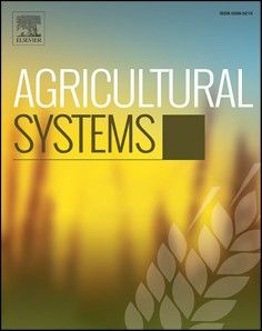
J.V. Silva et al. Agricultural Systems 198 (2022) 103383
Fig. 4. Distribution of farmers' actual yields (Ya) in comparison with the simulated potential yield (Yp) across different sowing dates in four irrigated lowland rice
areas in Southeast Asia. The simulated Yp for optimum sowing date and the highest yielding variety (Ypa) is indicated by the arrows. The simulated potential yield for
farmers' sowing dates and highest yielding variety (Ypb) is indicated by the solid line. Ypb was modelled using the rice varieties presented in Table 1. Codes: DS = dry
season, WS = wet season.
respectively (Fig. 3C). Differences between Ypa, Ypb, and Ypc during the the analysis had a significant effect on the efficiency yield gap during the
DS were negligible (Fig. 3C). The small sowing date and genetic yield DS, whereas farmers reporting a greater number of years of farming
gaps in the DS are the result of a relatively stable Ypb between October experience exhibited greater efficiency yield gaps during the WS
10 and December 17 (Fig. 4B), and to the fact that 82% of farmers used (Table 3). Farmers in Can Tho managed farms with an average of 2 ha
the same variety, c.v. Jasmine 85 (data not shown). and no larger than 5 ha (Fig. 6A) and rice income accounted for ca. 50%
During the 2015 WS, the mean Ypa in Can Tho was 10.1 t ha− 1, Ya of the total annual income for about half of the farmers surveyed
was 4.9 t ha− 1 and the yield gap between Ypa and Ya was 5.2 t ha− 1 (Fig. 6B).
(Fig. 3D; Suppl. Table S1). The yield gap was mostly explained by the
technology and efficiency yield gaps, which were 27% and 18% of Ypa,
respectively, while the resource yield gap was 6% of Ypa (Fig. 3D). The 4.3. Nakhon Sawan, Central Thailand
technology yield gap in the WS was equally explained by the sowing
date and the genetic yield gaps, which accounted for 15% of Ypa each Ypa during the 2013 DS in Nakhon Sawan was on average 9.2 t ha− 1
(Fig. 3D). The relatively large technology yield gap in the WS was the and Ya was on average 4.6 t ha− 1, which translated in a yield gap of 4.6 t
result of a sowing window spanning over 3 months, between March and ha− 1 (Fig. 3E; Suppl. Table S1). The small sample size during the DS did
May (Fig. 4B), and of eight rice varieties being used, with the most used not allow to disentangle efficiency and resource yield gaps, yet the yield
variety, OM 5451, being sown by 61% of the surveyed farmers (data not gap between Ypc and Ya accounted for 35% of Ypa and the technology
shown). yield gap accounted for 15% of Ypa (Fig. 3E). There was a wide sowing
N applied was the main driver of rice yield in Can Tho in both sea window during the DS spanning between November and January, with
sons, but there was also a positive effect of K applied on rice yield during considerable decreases in Ypb after December (Fig. 4C). High tempera
the WS (Table 3). For instance, increasing N by 1% increased rice yield tures, leading to heat stress, occurred during March and negatively
by 0.09 and 0.38% in the DS and WS, respectively (Table 3). N appli affected the Ypb of rice crops sown between January and February
cation rates ranged between 30 and 150 kg N ha− 1 in the WS and be (Suppl. Figs. S1 and S3).
tween 70 and 150 kg N ha− 1 in the DS (Fig. 5). This range of N During the 2013 WS, Ypa and Ya in Nakhon Sawan had an average
application rates corresponded to the steep slope of the curve charac value of 8.6 and 4.8 t ha− 1 respectively, corresponding to a yield gap of
terizing the yield response to N applied for the pooled data across the 3.8 t ha− 1 (Fig. 3F; Suppl. Table S1). The yield gap during the WS
four sites (Fig. 5). There was also a negative effect of P applied on rice explained by the efficiency, resource, and technology yield gaps
yield in the WS and rice yield was 17% greater for short-duration vari accounted for 12, 21, and 12% of Ypa, respectively (Fig. 3F). The length
eties than for long-duration varieties. None of the factors considered in of the sowing window in the WS was comparable to the DS, yet there was
much less variation in Ypb during the WS than in the DS (Fig. 4C). It was
9J.V. Silva et al. Agricultural Systems 198 (2022) 103383
Fig. 5. Rice yield response to N applied across four irrigated lowland rice areas in Southeast Asia. Panels (A) and (B) present rice yields in absolute terms during the
dry season (DS) and wet season (WS), respectively. Panels (C) and (D) present rice yield gap closure with actual yields shown as a proportion of the simulated
potential yield (Ypa) during the DS and WS, respectively. Each observation corresponds to one individual field in each of the four irrigated lowland rice areas. The
solid line depicts a quantile regression fitted to the 90th percentile of the pooled data and the dashed line in Panels (C) and (D) shows a relative yield gap closure of
80% of Ypa.
Fig. 6. Boxplots of farm size in ha (A) and share of rice income in total annual income in % (B) in four irrigated lowland rice areas in Southeast Asia. Data are pooled
for the wet and dry seasons in each site. Red diamonds indicate the mean. (For interpretation of the references to colour in this figure legend, the reader is referred to
the web version of this article.)
not possible to decompose the technology yield gap further for this site The drivers of rice yield variability in Nakhon Sawan were the use of
as only one rice variety was calibrated in ORYZA v3 (cf. Table 1). Yet, all herbicides and the difference in sowing date relative to the optimum
varieties used by farmers had a growth duration of 110–120 days (data sowing date identified with crop modelling (Table 3). Similarly to Bago,
not shown). fields where herbicides were used yielded 25% more than fields where
10J.V. Silva et al. Agricultural Systems 198 (2022) 103383
no herbicides were used but the latter accounted only to ca. 5% of the (2016), these results refer to both wet and dry season rice crops and
sampled fields (cf. Table 1). Moreover, one week deviation from the consider field-specific yield potentials, reflecting the highest yielding
optimal sowing date resulted in a 10% decrease in rice yield. There was varieties available to farmers and the optimal sowing dates within the
no statistically significant effect of N applied on rice yield in Nakhon range of sowing dates reported by farmers.
Sawan, which confirms the visual observations presented in Fig. 5 for Most of the yield gap for rice in Bago, Myanmar, was attributed to the
this site. Similarly to Can Tho, N application rates in the WS and in the resource yield gap, followed by the technology (sowing date) yield gap
DS ranged between 40 and 150 kg N ha− 1, which can be considered (Fig. 3A and B). Increasing input use, namely fertilizers, and proper
optimal for most fields (Fig. 5). None of the inefficiency effects consid weed control is thus necessary if yield gaps are to be narrowed in Bago
ered in the stochastic frontier analysis were identified as determinants of (Figs. 3A, B and 5; Thwe et al., 2019; Radanielson et al., 2019). N
the efficiency yield gap in this site (Table 3). Farmers in Nakhon Sawan application rates in Bago were well below 60 kg N ha− 1 in most fields,
had larger farm sizes than farmers at the other sites (Fig. 6A), with an confirming the low amounts of inputs used and the low level of yield gap
average farm size of ca. 5 ha and about half of the farmers surveyed closure in this site (Fig. 5). Despite the small amount of N applied, other
reporting farm sizes above 4 ha. Similar to Can Tho, rice income factors (e.g., pests, diseases and weeds, balanced fertilization, or timing
accounted for ca. 60% of the total annual income (Fig. 6B). of N application) may also be reducing or limiting rice yield. Improve
ments in pest, disease, and nutrient management are likely to be needed,
4.4. Yogyakarta, Java, Indonesia in tandem with increases in N applied, for intensifying rice production in
this site. The levels of fertilizer use and rice yield observed in Bago are
During 2014 DS, Ypa in Yogyakarta was on average 11.1 t ha− 1, Ya comparable to those observed in the 1970s for rice crops in Central
was 4.5 t ha− 1 and the respective yield gap between Ypa and Ya was 6.6 t Luzon, the Philippines (Kajisa and Payongayong, 2011; Laborte et al.,
ha− 1 (Fig. 3G; Suppl. Table S1). Most of the yield gap in the DS was 2012). Moreover, narrowing the sowing date yield gap through early
attributed to the technology yield gap (34% of Ypa) and to the efficiency sowing in the DS or late sowing in the WS within the three-month
yield gap (25% of Ypa; Fig. 3G). The technology yield gap was mostly sowing window also offers opportunities to increase rice yield
attributed to the sowing date yield gap in the DS with the genetic yield (Fig. 4A). The sowing date yield gap estimated in Bago also indicates
gap contributing to less than 5% of Ypa (Fig. 3G). Rice was sown across a high climatic risk for rice cropping in the region within the sowing
five-month period during the DS (between March and August; Fig. 4D), window reported by the farmers.
with the sowing date yield gap representing 32% of Ypa (Fig. 3G). Rice yield gaps in Yogyakarta, Indonesia, were mostly attributed to
Farmers who planted between June and August were likely to be those efficiency and technology (sowing date) yield gaps (Fig. 3G and H).
with irrigation available all year, who either planted late or planted a Resource yield gaps were negligible in this site during the DS, where
second DS rice crop that was not differentiated in this analysis from the indeed excessive N application rates were observed in both DS and WS
early DS crop, as this was not clarified during the farm survey. (Fig. 5). Such large N application rates are a typical feature of high-
In the 2014 WS, slightly smaller yields and yield gaps were observed yielding cropping systems (Nayak et al., 2022; Cui et al., 2018; Silva
in Yogyakarta than in the DS: Ypa and Ya were on average 10.4 and 4.8 t et al., 2017a, 2017b). The fairly large resource yield gap observed in the
ha− 1, respectively, corresponding to a yield gap of 5.6 t ha− 1 (Fig. 3H; WS was surprising given the excessive N rates observed in farmers' fields
Suppl. Table S1). The yield gap was mostly explained by the resource (Fig. 5), most likely due to limitations in the stochastic frontier analysis
yield gap (19% of Ypa) and by the efficiency yield gap (11% of Ypa; (see Section 5.3). Yet, farmers reported yield losses due to blast and
Fig. 23H). The technology yield gap in the WS was also mostly attributed bacterial leaf light during this WS, possibly due to excessive use of N,
to the sowing date yield gap (Fig. 2H). During the WS, rice was sown which might explain why YTEx was smaller than Ypc (Figs. 3H). Thus,
between October and January (Fig. 4D) and the sowing date yield gap further increases in rice yield in this site must be derived through a
explained about 10% of Ypa (Fig. 3H). combination of reductions in applied N (Fig. 5) and increases in
N applied had a significant positive effect on rice yield, with a 1% resource-use efficiency via better timing, space, and form of the inputs
increase in N applied resulting in ca. 0.10% increase in rice yield during applied (Fig. 3G and H), and adaptive seasonal management such as
both seasons, respectively (Table 3). There was also a positive effect of P shifting of sowing dates (Fig. 4D). The sowing window in the DS was
applied on rice yield during the DS (Table 3). Across the four sites, N wide (Fig. 4D) as farmers were sowing following the irrigation schedule
application rates were greatest in Yogyakarta, ranging between 75 and established by the national irrigation authority. Optimization of sowing
350 kg N ha− 1 (Fig. 5). N application rates beyond 180–200 kg N ha− 1 dates in the DS is only feasible then if the irrigation water scheduling can
translated into marginal, or even negative, rice yield response to N be adapted accordingly. Late DS sowing and early WS sowing also pre
applied when considering the pooled data (Fig. 5). Such negative yield sented a risk of heavy rainfall at harvest which has a significant effect in
response to N applied were not captured in the stochastic frontier securing timely harvesting and grain quality. Future studies accounting
analysis (Table 3) most likely because squared terms and interactions for the impact of climatic risk on harvest time and grain quality are
between variables were not considered in the fitted models. The effi needed to formulate adapted recommendations contributing to reduce
ciency yield gap decreased with increasing share of rice income to total the sowing date yield gap in Yogyakarta. Moreover, intensification using
annual income (Table 3), meaning that inputs applied were better three crops per year in Yogyakarta is limited by water availability during
managed in farms relying more on rice as a source of income. Indeed, the latter half of the dry season.
rice income accounted for ca. 70% of the total annual income in The efficiency, resource, and technology (sowing date) yield gap
Yogyakarta (Fig. 6B), despite the extremely small farm sizes at this site contributed equally to the rice yield gap in Nakhon Sawan, Thailand,
(Fig. 6A). during the WS (Fig. 3F). The relative contribution of the intermediate
yield gaps is comparable to that observed for rice farming in Central
5. Discussion Luzon, Philippines (Silva et al., 2017a, 2017b), as too the level of yield
gap closure (ca. 50% of Ypa). Efficiency and resource yield gaps had a
5.1. Drivers of rice yield gaps in Southeast Asia similar magnitude in Nakhon Sawan (Fig. 3E and F), and herbicide use
was an important factor associated with narrowing the resource yield
Crop modelling was combined with the analysis of farm survey data gap (Table 3). Earlier sowing is also likely to increase rice yields,
to estimate and decompose rice yield gaps across four sites in Southeast particularly during the DS (Fig. 4C). Indeed, long-term analysis of rice
Asia (Fig. 2). The rice yield gap was largest in Bago (75% of Ypa), fol yield response to temperature indicated that late sowing of DS rice
lowed by Yogyakarta (57% of Ypa), Nakhon Sawan (47% of Ypa) and Can during the months of January–March resulted in greater risks of spikelet
Tho (44% of Ypa; Figs. 2 and 5). Building upon the study by Stuart et al. sterility due to temperature stress (Suppl. Fig. S3). Increasing rice
11You can also read