Activity distribution of comet 67P/Churyumov-Gerasimenko from combined measurements of non-gravitational forces and torques
←
→
Page content transcription
If your browser does not render page correctly, please read the page content below
Astronomy & Astrophysics manuscript no. Attree_NGA_Paper2_LanguageEdited                                              ©ESO 2023
                                               January 13, 2023

                                                 Activity distribution of comet 67P/Churyumov-Gerasimenko
                                                from combined measurements of non-gravitational forces and
                                                                            torques
                                                 N. Attree1 , L. Jorda2 , O. Groussin2 , J. Agarwal1 , R. Lasagni Manghi3 , P. Tortora3, 4 , M. Zannoni3, 4 , and
                                                                                                 R. Marschall5

                                                    1
                                                        Institut für Geophysik und extraterrestrische Physik, Technische Universität Braunschweig, Mendelssohnstr. 3, 38106
                                                        Braunschweig, Germany (e-mail: n.attree@tu-braunschweig.de)
                                                    2
                                                        Aix Marseille Univ, CNRS, CNES, Laboratoire d’Astrophysique de Marseille, Marseille, France
                                                    3
arXiv:2301.04892v1 [astro-ph.EP] 12 Jan 2023

                                                        Alma Mater Studiorum - Università di Bologna, Dipartimento di Ingegneria Industriale, Via Fontanelle 40, I-47121
                                                        Forlì, Italy
                                                    4
                                                        Alma Mater Studiorum - Università di Bologna, Centro Interdipartimentale di Ricerca Industriale Aerospaziale, via
                                                        Baldassarre Carnaccini 12, I-47121, Forlì, Italy
                                                    5
                                                        CNRS, Laboratoire J.-L. Lagrange, Observatoire de la Côte d’Azur, Boulevard de l’Observatoire, CS 34229 - F 06304
                                                        NICE Cedex 4, France

                                                    January 13, 2023

                                                                                                           ABSTRACT

                                                    Aims. Understanding the activity is vital for deciphering the structure, formation, and evolution of comets. We inves-
                                                    tigate models of cometary activity by comparing them to the dynamics of 67P/Churyumov-Gerasimenko.
                                                    Methods. We matched simple thermal models of water activity to the combined Rosetta datasets by fitting to the total
                                                    outgassing rate and four components of the outgassing induced non-gravitational force and torque, with a final manual
                                                    adjustment of the model parameters to additionally match the other two torque components. We parametrised the
                                                    thermal model in terms of a distribution of relative activity over the surface of the comet, and attempted to link this
                                                    to different terrain types. We also tested a more advanced thermal model based on a pebble structure.
                                                    Results. We confirm a hemispherical dichotomy and non-linear water outgassing response to insolation. The southern
                                                    hemisphere of the comet and consolidated terrain show enhanced activity relative to the northern hemisphere and
                                                    dust-covered, unconsolidated terrain types, especially at perihelion. We further find that the non-gravitational torque
                                                    is especially sensitive to the activity distribution, and to fit the pole-axis orientation in particular, activity must be
                                                    concentrated (in excess of the already high activity in the southern hemisphere and consolidated terrain) around the
                                                    south pole and on the body and neck of the comet over its head. This is the case for both the simple thermal model
                                                    and the pebble-based model. Overall, our results show that water activity cannot be matched by a simple model of
                                                    sublimating surface ice driven by the insolation alone, regardless of the surface distribution, and that both local spatial
                                                    and temporal variations are needed to fit the data.
                                                    Conclusions. Fully reconciling the Rosetta outgassing, torque, and acceleration data requires a thermal model that
                                                    includes both diurnal and seasonal effects and also structure with depth (dust layers or ice within pebbles). This shows
                                                    that cometary activity is complex. Nonetheless, non-gravitational dynamics provides a useful tool for distinguishing
                                                    between different thermophysical models and aids our understanding.
                                                    Key words. comets: general, comets: individual (Churyumov-Gerasimenko), planets and satellites: dynamical evolution
                                                    and stability

                                               1. Introduction                                                    formation in the early Solar System. Whether cometary
                                                                                                                  nuclei, and by extension planets, formed from the gravi-
                                                                                                                  tational collapse of clouds of centimetre-sized pebbles (as
                                               Comets are amongst the most primordial Solar System ob-            proposed in Blum et al. 2017) or by continual collisional
                                               jects. They formed directly from the protoplanetary disc           growth (Davidsson et al. 2016) has direct implications for
                                               and survived mostly unaltered for much of their lifetimes          the structure and strength of the near-surface material that
                                               in the outer Solar System. They are therefore vital targets        controls outgassing.
                                               for our understanding of planet formation and the history
                                               of the early Solar System. Upon entering the inner Solar
                                               System, comets are heated by the Sun and undergo ac-                   In addition to being directly observable, the outgassing
                                               tivity; that is, ices are sublimated and gas and dust are          produces a reaction force on the nucleus that can alter its
                                               ejected. Cometary activity poses open questions related to         trajectory (as first recognised by Whipple 1950 and de-
                                               the structure, composition, and thermophysical properties          scribed by Marsden et al. 1973) and rotation state (see
                                               of the nucleus material. This is directly connected to their       Samarasinha et al. 2004). Measuring the changing orbits
                                                                                                                                                       Article number, page 1 of 13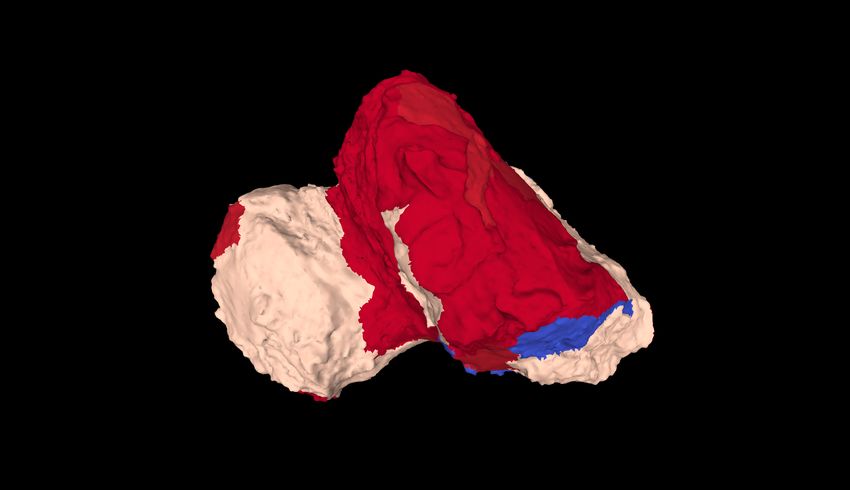
A&A proofs: manuscript no. Attree_NGA_Paper2_LanguageEdited

and spins of comets therefore provides a useful insight into      tal production measurements and the NGA. However, our
the the micro-physics of the activity mechanism.                  model was limited by not considering the other components
    Many thermophysical models have been proposed to ex-          of the NGT (i.e. the change in the spin axis orientation, as
plain the activity (see recent examples by Fulle et al. 2019,     well as its magnitude), and by a rather nonphysical way
Gundlach et al. 2020, and Davidsson 2021), and these can          of splitting the surface into areas of differing activity. Ad-
be compared to the outgassing rates of observed comets. In        ditionally, discontinuities in the cometary heliocentric tra-
particular, comet 67P/Churyumov-Gerasimenko (67P here-            jectory reconstructed by the European Space Operations
after) provides an excellent dataset because it was visited by    Centre that arose because the NGA was excluded from the
the Rosetta spacecraft between 2014 and 2016. The space-          operational dynamical model, have complicated the anal-
craft collected detailed measurements of the size, shape,         ysis by making it difficult to extract smooth acceleration
surface properties, and time-varying rotation state and out-      curves.
gassing of the nucleus. Finding the distribution of activity          Kramer & Läuter (2019) addressed this problem by per-
across the nucleus of 67P that fits the various measurements      forming their own N-body integrations with a model fol-
of the total outgassing rate best (Hansen et al. 2016; Mar-       lowing Yeomans & Chodas (1989) and varying initial con-
shall et al. 2017; Combi et al. 2020; Läuter et al. 2020, etc.)   ditions. They then fitted a smoothed, interpolated curve to
has produced several so-called activity maps (e.g. Marschall      the residuals to extract time-varying NGA curves, but they
et al. 2016, 2017; Läuter et al. 2020, ), which are often ex-     did not compare them to a full thermal model. In a separate
pressed as an effective active fraction (EAF) relative to a       paper (Kramer et al. 2019), the authors did compare a phys-
pure water-ice surface. When examining only the summed            ical thermal model, again using the EAF formalism, to both
total outgassing, however, there is always a degeneracy in        the rotation rate and axis orientation data. Similarly to our
the retrieved activity distribution (Marschall et al. 2020),      results, their results also required a relatively higher EAF in
whilst, at the same time, the effects of seasonal changes in      the southern than in the northern hemisphere, as well as an
insolation and dust cover across the surface of 67P are com-      enhanced outgassing response to insolation around perihe-
plicated (Keller et al. 2017; Cambianica et al. 2021). Com-       lion to fit the data. Kramer & Läuter (2019) noted that the
paring the effects of a model outputted non-gravitational         NGT is much more dependent on the spatial distribution
acceleration (NGA) and torque (NGT) to the dynamics of            of activity than the NGA.
67P can provide a further constraint on the model parame-             Since then, two additional reconstructions of the
ters and on our understanding of the activity (Attree et al.      Rosetta/67P trajectory have been performed (Farnocchia
2019; Kramer et al. 2019; Kramer & Läuter 2019; Mottola           et al. 2021; Lasagni Manghi et al. 2021). Farnocchia et al.
et al. 2020).                                                     (2021) used a rotating-jet model following Sekanina (1993)
    Simple NGA models, such as those by Marsden et al.            to fit ground-based astrometric observations and radio-
(1973) and Yeomans & Chodas (1989), parametrise the               ranging measurements before and after perihelion (where
acceleration using variables scaled to a general water-           the spacecraft NGAs are smaller and the range accuracy is
production curve, and therefore provide limited insight           higher). Lasagni Manghi et al. (2021), on the other hand,
into the physics of the activity on an individual comet.          used the full Rosetta two-way range and differential one-
More complex models (following from Sekanina 1993) re-            way range (∆DOR) dataset, also including low-accuracy
late the observed NGA and NGT to the outgassing via               data close to perihelion. They tested various NGA models,
a thermal model and some distribution of ices or active           including a rotating-jet model, and found a best-fit tra-
areas across the nucleus surface. If independent measure-         jectory using an empirical, stochastic acceleration model.
ments of this distribution and/or the outgassing rate can         Both of these works produced acceleration curves to which
be made, then cometary masses and spin axes can be mea-           a thermal model can be compared.
sured from ground-based observations, as was achieved for             Davidsson et al. (2022) did just that by comparing
67P (Davidsson & Gutiérrez 2005; Gutiérrez et al. 2005).          the output of a more complex thermal model (NIMBUS;
Rosetta then provided both the detailed outgassing data           Davidsson 2021) to the acceleration curves of Farnocchia
mentioned above, as well as precise measurements of the           et al. (2021) and Kramer & Läuter (2019). They found rel-
nucleus position and rotation via radio-tracking and op-          atively good agreement without fitting, but had to vary
tical navigation. As summarised in Mottola et al. (2020),         several model parameters (e.g. the sublimation-front depth
various attempts have been made to compare thermal mod-           and the gas diffusivity) between the northern and south-
els to the NGA and NGT forces of 67P (Keller et al. 2015;         ern hemispheres and pre- and post-perihelion, in order to
Davidsson et al. 2022) and to fit its non-gravitational tra-      match the outgassing data. This reinforces the ideas of a
jectory (Kramer & Läuter 2019), rotation state (Kramer            hemispheric dichotomy and time-dependent thermophysi-
et al. 2019), and both in combination with outgassing (At-        cal properties, and it also demonstrates the complicated
tree et al. 2019).                                                nature of trying to model the full thermophysical system of
    In Attree et al. (2019), our previous paper on this topic,    sublimation, gas flow, and dust.
we used the EAF formalism to fit surface distributions to             These studies show the usefulness of considering the
the observed Earth-comet range (the most accurate compo-          non-gravitational dynamics. No study has analysed the full
nent of the comet ephemeris, based on the spacecraft radio        six components of NGA and NGT simultaneously, how-
tracking), total gas production (measured by ROSINA, the          ever (we analyse all six here, but only four are included in
Rosetta Spectrometer for Ion and Neutral Analysis; Hansen         the formal fitting procedure), and several other weaknesses
et al. 2016), and the change in spin rate (z component of         exist, such as nonphysical surface distributions or compli-
the torque, measured as part of the nucleus shape recon-          cated descriptions leading to unfitted models. It is per-
struction; Jorda et al. 2016). We found that a large EAF in       tinent, therefore, to re-examine the full non-gravitational
the southern hemisphere of the comet, as well as an increase      dynamics of 67P with a simple thermal model that can
in EAF around perihelion, were needed to fit both the to-         be parametrised in terms of real surface features while be-
Article number, page 2 of 13
N. Attree et al.: Activity distribution of comet 67P

ing easily compared with more complicated models. This            ity assumes that the gas equilibrates with the dusty surface,
is what we attempt to do here, bearing in mind that the           and this means that our derived EAF values may be lower
aim is not to find the full description of cometary activity,     estimates compared with some other thermal models.
but a model that adequately describes the data and points             The N-body integration was performed using the open-
towards the underlying physics.                                   source REBOU N D code1 (Rein & Liu 2012), complete
    The rest of this paper is organised as follows: in Sec-       with full general relativistic corrections (Newhall et al.
tion 2 we describe how we updated the model of Attree             1983) as implemented by the REBOU N Dx extension pack-
et al. (2019) for use here. In Section 3 we describe three        age2 , and including all the major planets as well as Pluto,
different parametrisations of the surface activity distribu-      Ceres, Pallas, and Vesta. Objects were initialised with their
tion and their results in the model fit. These results are        positions and velocities in the J2000 ecliptic coordinate
discussed, with reference to a run with the more advanced         system according to the DE438 Solar System ephemerides
thermal model of Fulle et al. (2020) in Section 4, before we      (Standish 1998), with 67P given its initial state vector
conclude in Section 5.                                            from the new Rosetta trajectory reconstruction of Lasagni
                                                                  Manghi et al. (2021) (Table A.1). The system was then inte-
2. Method                                                         grated forward in time from t = −350 to +350 days relative
                                                                  to perihelion, using the IAS15 integrator (Rein & Spiegel
We followed the method of the first paper (Attree et al.          2015) and the standard equations of motion, with the addi-
2019) by first calculating surface temperatures over a shape      tion of a custom acceleration, aN G , for 67P, provided by our
model of 67P (SHAP7; Preusker et al. 2017) with a simple          model. The Earth-comet range, which is the most accurate
energy-balance thermal model and then computing the re-           component of the comet trajectory, was computed for com-
sulting non-gravitational forces and torques and implement-       parison with the reconstructed trajectory (extracted using
ing them in an N-body integration. The model was then             the SpiceyP y Python package; Annex et al. 2020).
optimised by scaling the relative activity of various areas
of the shape model up and down, minimising the residuals               A bounded least-squares fit to the residuals was then
to the observed datasets: the Earth-comet range (i.e. the         performed using standard methods implemented in Scien-
scalar projection of the three-dimensional comet position in      tific Python whilst varying the EAF parameters. When
the Earth-comet direction, R, with NR = 1000 data points)         forming the overall objective function to be minimised (see
or the directly extracted NGAs from Lasagni Manghi et al.         Eqns. 9 and 10. in Attree et al. 2019), the datasets were
(2021) (with NN GA = 17000 data points in each of the three       weighted by a factor λ so that each contributed roughly the
components); the total gas production (NQ = 787, Hansen           same to the overall fit (see Table 1). The datasets used in all
et al. 2016); and the spin-axis (z) aligned component of the      fits were the model outputted total outgassing rate and the
torque (NTz = 1000, Jorda et al. 2016). Additionally, we          z component of the torque, both with λQ = λTz = 1. Fur-
now also computed the change in the orientation of the ro-        thermore, in some fits, we then used the computed Earth-
tation axis (Kramer et al. 2019) and used this as an output       comet range (with λR = 0.02), while in others, we directly
to compare different models.                                      compared to the three components of the NGA extracted by
     The thermal model computes the surface energy-               Lasagni Manghi et al. (2021) in the cometocentric radial-
balance, taking insolation, surface thermal emission, sub-        transverse-normal frame (radial to the Sun, r̂, tangential
limation of water ice, projected shadows, and self-heating        to the orbit, t̂, and normal to it). In this case, the inte-
into account (see Attree et al. 2019 for details). Heat con-      gration was only performed once at the end to check the
duction into the nucleus is neglected for numerical reasons,      Earth-comet range, but the weighting was zero in the fit
but is small because of the low thermal inertia of the comet      (λR = 0), while λNGA = 1. Performing the N-body inte-
(Gulkis et al. 2015). Heat conduction would mainly affect         gration only once speeds the process up by several times,
night-time temperatures, which are very low and contribute        with individual runs taking a few minutes and fits taking
little to the outgassing (but see the discussion in Section 4).   up to a day, depending on the parameters. All parameters
Again for numerical reasons, surface temperatures are cal-        were interpolated to the observational data sampling-times
culated roughly once every 10 days for a full 12.4 hour ro-       using the Fourier method described below.
tation, and the derived quantities are interpolated (see de-          We first confirm that the Lasagni Manghi et al. (2021)
tails below) to produce smooth curves over the full mission       accelerations match the real comet trajectory well when
period of about two years. Surface temperatures are each          they are input into our N-body integration, and they re-
computed twice, once assuming an effective active fraction        cover the Earth-comet range to within a few hundred me-
EAF = 0 (i.e. pure grey-body dust surface), and once with         tres. This residual, which is most likely the result of the
EAF = 1 (i.e. sublimation from a pure water-ice surface),         different integration techniques and perturbing bodies we
and the temperatures and sublimation rates are saved. In          used, is well below the uncertainty of our thermal model
the fitting process, the pure water-ice sublimation rate is       runs.
then scaled by a variable EAF and is used, along with
the sublimation gas velocity calculated from the zero-ice            Previously, the x and y components of the torque vector
surface temperature, to compute the outgassing force per          were discarded, but they were now used when we calculated
facet. The momentum coupling parameter was assumed to             the changes in pole orientation. In principle, the rates of
be η = 0.7 (Attree et al. 2019). Torque per facet was also        change of the angular velocity (Ω) of the comet around its
calculated here using the “torque efficiency” formalism used      three principal axes can be related (see e.g. Julian 1990) to
before (Keller et al. 2015), where τ is the facet torque ef-
ficiency or moment arm, which is a geometric factor that
was computed once at the beginning of the run. The use of         1
                                                                      http://rebound.readthedocs.io/en/latest/
the higher zero-ice temperature for the gas thermal veloc-        2
                                                                      http://reboundx.readthedocs.io/en/latest/index.html

                                                                                                    Article number, page 3 of 13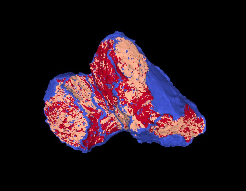
A&A proofs: manuscript no. Attree_NGA_Paper2_LanguageEdited
the torque components by
+Z
Ix Ω˙x = (Iy − Iz )Ωy Ωz + Tx , -Z
Iy Ω˙y = (Iz − Ix )Ωx Ωz + Ty , (1)
Iz Ω˙z = (Ix − Iy )Ωx Ωy + Tz ,
where Ix = 9.559 × 10¹⁸ , Iy = 1.763 × 10¹⁹ , and Iz =
1.899 × 10¹⁹ kg m2 are the moments of inertia derived from
the shape model assuming a constant density of 538 kg m−3
(Preusker et al. 2017), and to the pole orientation right
ascension, RA, and declination, Dec, by
−Ωy cos(ψ) − Ωx sin(ψ)
ψ̇ = + Ωz ,
tan(θ)
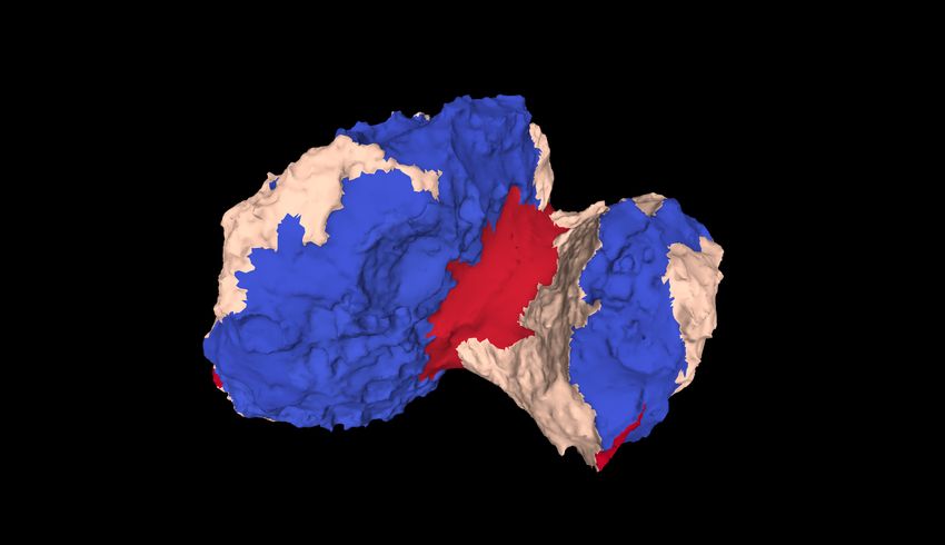
Ωy cos(ψ) + Ωx sin(ψ) (2) Fig. 1. Peak effective active fraction at perihelion for solution
φ̇ = , C, mapped onto the shape model.
sin(θ)
θ̇ = Ωx cos(ψ) − Ωy sin(ψ),
via the Euler angles φ = π/2 + RA, θ = π/2 − Dec, and ψ.
In practice, the fact that our model runs over individual So th -
Region 1
rotations separated by gaps means that the torque curves 0.4 Region 2
are discontinuous and cannot be directly integrated. We Hathor
therefore followed the technique of Kramer et al. (2019) and Hapi
So th +
Active Fraction
applied a Fourier analysis to the torque curves. The method 0.3
proceeds by i) extracting the torque over a single rotation
as a function of the sub-solar longitude, using Kramer et al.
0.2
(2019) Eqns. 26, 27, ii) computing the Fourier transform as
a function of sub-solar longitude using Eqn. 23, iii) inter-
polating the Fourier terms as smooth curves over the full 0.1
Rosetta period; Eqn. 24, and iv) reconstructing the torque
at a chosen time by the inverse Fourier transform; Eqn.
25. This allows the calculation of a smoothly interpolated 0.0
torque value at any given time, Tx,y,z (t), for use in the ro- −400 −300 −200 −100 0 100 200 300 400
tation equations (1). Days from Perihelion
The set of simultaneous differential equations given by
Eqns. 1 and 2 was then integrated using standard func- Fig. 2. Time-varying effective active Fraction for solution C.
tions in Scientific Python and the initial conditions RA =
69.427◦ , Dec = 64.0◦ , and ψ = 330.703◦ at t = −377.22
days relative to perihelion (Kramer et al. 2019) for the pe- two southern super-regions split on a per-facet basis by the
riod t = [−377.22 : 402.48], corresponding to the duration sign of the z component of the torque efficiency (i.e. south
of the Rosetta measurements. The resulting RA(t), Dec(t) positive with τz > 0 and south negative with τz < 0).
values were not used in the fit due to technical limita- This splitting was the only way in which a satisfactory fit
tions, but were directly compared with the observations as to the z torque (i.e. rotation-rate data) could be achieved,
a model output. but it remains somewhat artificial. Figure 1 shows the best-
fit solution achieved here, mapped onto the shape model.
This shows the discontinuous and patchy appearance of the
3. Results southern super-regions, as well as the north-south EAF di-
chotomy and activity in Hapi (the light blue area in the
3.1. Model C northern neck region).
We began by rerunning the best-fit model of the previous We optimised this model again here and, with a slightly
paper, designated model C in Attree et al. (2019). This differing procedure for sampling and interpolating the com-
model parametrised the activity distribution by splitting putational output, produced very similar results to before,
the surface into the 26 regions, defined by Thomas et al. with no significant improvement in the fit. Next, we in-
(2015) (see their figures for maps), and then grouping them stead fit the model directly to the Lasagni Manghi et al.
into five super-regions following Marschall et al. (2016)(see (2021) NGA curves as described above, producing the best-
Figure 4 in Attree et al. 2019), before finally splitting the fit solution shown mapped onto the shape-model in Figure
Southern super-region into two (see Figure 17 in Attree 1 (where the values shown are peak EAF, the maximum
et al. 2019) and allowing these to vary their EAF with time. value for all times), and with time in Figure 2. The out-
With 6 super-regions and the 6 time-variation parameters, put is very similar to the previous solution in Attree et al.
there are a total of 12 free parameters in this model. These (2019), but Figure 2 shows an even more pronounced spike
super-regions consist of region 1, covering the equatorial ar- in EAF around perihelion than before.
eas; region 2, covering the base of the comet body and top The model fits are shown in the orange curves in Fig-
of the head; the individual regions Hathor and Hapi; and ures 3, 4, and 5, with the fit statistics in the first line of
Article number, page 4 of 13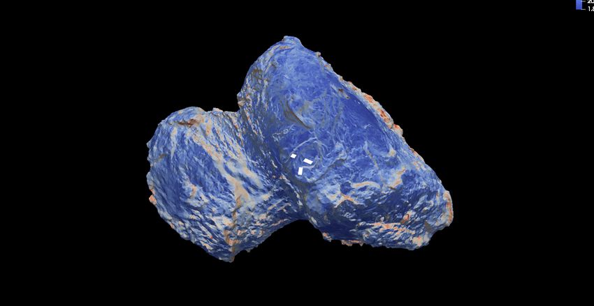
N. Attree et al.: Activity distribution of comet 67P

                                                                                                                          1e7
                                                                                                                    1.0
                                          Model C                                                                                                                           Observed
                                          Model D                                                                   0.8                                                     Model C
                             1028         Model E                                                                                                                           Model D
     Ou gassing Ra e (s−1)

                                          Observed                                                                  0.6                                                     Model E

                                                                                                    Tor ue (Nm)
                             1027                                                                                   0.4

                                                                                                                    0.2

                             1026
                                                                                                                    0.0

                                    −300      −200      −100       0        100     200                                         −300   −200    −100       0     100     200     300
                                                   Days from Perihelion                                                                       Days from Perihelion
    Fig. 3. Observed total gas production (ROSINA values from                                     Fig. 5. Smoothed observed z component of the torque com-
    Hansen et al. 2016) compared to solutions C, D, and E.                                        pared to solutions C, D, and E. The grey area represents the 1σ
                                                                                                  uncertainty (see Attree et al. 2019 for details).

                             200                                                                                          1e 9
                                          Model C                                                                   1.0
                             150          Model D                                                                                                                           Observed
                                          Model E                                                                                                                           Model C
Range Residuals (km)

                             100                                                                                    0.8                                                     Model D
                              50                                                                                                                                            Model E
                                                                                                   NGA r (AU d 2)

                                0                                                                                   0.6

                              50
                                                                                                                    0.4
                             100
                             150                                                                                    0.2
                             200
                                                                                                                    0.0
                                    300      200      100      0   100      200   300
                                                   Days from Perihelion                                                         300    200     100    0       100     200     300     400
                                                                                                                                              Days from Perihelion
    Fig. 4. Observed minus computed Earth-comet range, R, for
    solutions C, D, and E.                                                                        Fig. 6. Observed radial acceleration in the comet (r̂, t̂, n̂) frame
                                                                                                  with the 5σ uncertainty (from Lasagni Manghi et al. 2021), com-
                                                                                                  pared to solutions C, D, and E. Higher-order Fourier terms cor-
                                                                                                  responding to daily oscillations are omitted for clarity, but are
    Table 1. The z torque (Fig. 5) and total gas production                                       included in the fit.
    from ROSINA (Fig. 3) are reasonably well fit, with the
    perihelion peak-values matched, but with a slightly differ-
    ing shape around the inbound equinox roughly 100 days                                             When the pole orientation was calculated, as shown in
    before perihelion. An improvement in the trajectory fit is                                    the orange curve of Figure 9, it was a very poor fit to the
    attained, with the new RMS residual value of 34 km re-                                        data, moving off in the opposite direction to the observed
    duced from the previously achieved 46 km. The shape of                                        changes. This demonstrates that the problem is ill-posed
    the curve is similar.                                                                         with multiple solutions, and it also highlights the useful-
        The orange curves in Figures 6, 7, and 8 show the in-                                     ness of including the RA, Dec pole measurement to help
    dividual acceleration curves in the cometocentric (r̂, t̂, n̂)                                distinguish between different models that fit the other data
    frame compared to the values extracted by Lasagni Manghi                                      equally well.
    et al. (2021). The radial component makes up the bulk of
    the acceleration and is reasonably well matched by model                                      3.2. Model D
    C, with the peak value being ∼ 50% too high. The normal
    and tangential components are of smaller magnitude and                                        We now proceed with a more physically meaningful model.
    are reasonably well fit; the secondary, negative peak of the                                  This was constructed using the list of 71 sub-regions de-
    tangential component after perihelion is the worst area of                                    fined in Thomas et al. (2018) (see the reference for maps of
    the fit. The remaining 34 km residuals to the observed tra-                                   their location). We again created super-regions by collecting
    jectory most likely stem from our inability to fit this area                                  these sub-regions, but this time, by placing them into one of
    of the tangential acceleration, combined with the too large                                   the five morphological categories of Thomas et al. (2015):
    radial component peak.                                                                        ‘dust-covered terrains’ (Dust for short), ‘brittle materials
                                                                                                                                                              Article number, page 5 of 13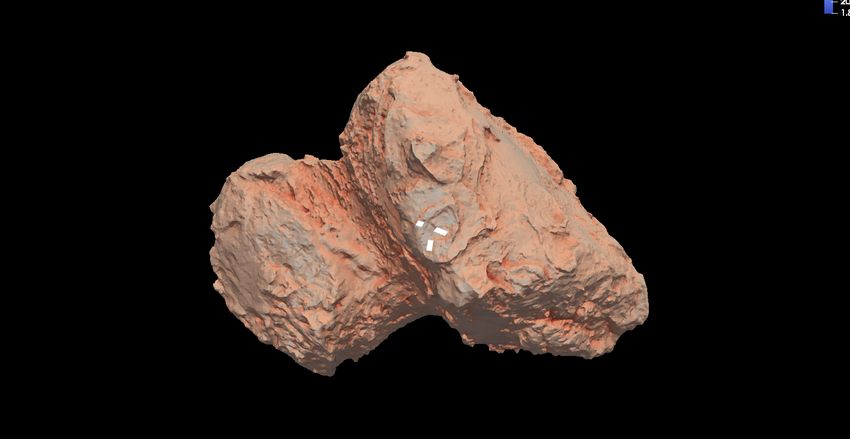
A&A proofs: manuscript no. Attree_NGA_Paper2_LanguageEdited

 Table 1. Fit statistics for best-fit models C, D, and E, and the two unfitted versions of F.

                                   Solution               Weighting                                                            χ2
                                                    λQ   λTz   λR   λNGA             R       Q                        Tz    NGAr       NGAt     NGAn      Obj
                                   C                 1    1     0     1             34.1    4.53                     1.36    1.18       1.32     0.44     1.20
                                   D                 1    1   0.02    0             88.8    3.60                     1.10    2.00       1.60     0.90     2.35
                                   E                 1    1   0.02    0            83.4     3.75                     0.77   1.78       1.58      0.89     2.22
                                   F dust SH         -    -     -     -            324.5    4.62                     2.09    4.12       1.71     1.01       -
                                   F ice SH          -    -     -     -            459.2    5.64                     3.02    2.22       1.63     1.00       -
 Notes. Model E is highlighted as the preferred solution. The model outputs (water production rate, z component of NGT, and
 the three components of NGA) are compared to the observations, producing the χ2 statistics, which are then weighted according
 to the λ values and combined in the objective function (Eqns. 9 and 10. in Attree et al. 2019) to produce the combined fit statistic
 Obj. All values are dimensionless, although the range values R correspond one-to-one to kilometers.

                           1e 10                                                                             65.50
                     2.0                                              Observed                               65.25
                                                                                                                            M del C
                                                                      Model C                                               M del D
                     1.5                                              Model D                                65.00          M del E
                                                                      Model E                                               Observed
NGA t (AU d 2)

                     1.0                                                                   Declinati n (∘)   64.75

                                                                                                             64.50
                     0.5                                                                                     64.25

                     0.0                                                                                     64.00

                                                                                                             63.75
                     0.5
                                                                                                             63.50

                              300     200     100    0    100   200    300   400                                      67      68        69       70       71     72
                                            Days from Perihelion                                                                    Right Ascensi n (∘)
 Fig. 7. Observed tangential acceleration in the comet (r̂, t̂, n̂)                          Fig. 9. Observed pole orientation (Ra, Dec) compared to solu-
 frame compared to solutions C, D, and E.                                                    tions C, D, and E. The thickness of the model lines is due to the
                                                                                             daily oscillations. Error bars are plotted for the observations,
                                                                                             but are small at this scale.

                           1e 10
                                                                                             tested in both the categories to which their descriptions
                     3.5                                              Observed               could apply, without altering our results significantly. The
                     3.0
                                                                      Model C                Rock and Smooth terrain types both cover significant ar-
                                                                      Model D                eas of the southern hemisphere and following the results
                     2.5                                              Model E                of the first paper, we therefore allowed their EAFs to vary
    NGA n (AU d 2)

                     2.0                                                                     with time in the same way as for model C. The facets in
                                                                                             each super-region all have the same EAF (either constant or
                     1.5                                                                     time-varying), regardless of the hemisphere in which they
                                                                                             are located. With five regions and 6 time-variation param-
                     1.0                                                                     eters, there are 11 parameters in total for this model, des-
                     0.5                                                                     ignated ‘model D’.
                                                                                                 Figure 10 shows the peak activity in our best-fit solution
                     0.0                                                                     for model D mapped onto the shape model, and Fig. 11
                                                                                             shows the time variation. High activity is again favoured
                              300     200     100    0    100   200    300   400
                                            Days from Perihelion                             in the southern hemisphere, with the Rock and Smooth
                                                                                             regions seeing much higher activity than the Dusty, Brittle,
 Fig. 8. Observed normal acceleration in the comet (r̂, t̂, n̂) frame                        and Depression regions, especially around perihelion.
 compared to solutions C, D, and E.                                                              Model D is shown as green curves in Figures 3 - 9. The fit
                                                                                             statistics are again shown in Table 1. This model produces
                                                                                             a similar, if slightly improved, fit to the total outgassing
 with pits and circular structures’ (Brittle), ‘large-scale de-                              measurements, while slightly degrading the trajectory and
 pressions’ (Depression), ‘smooth terrains’ (Smooth), and                                    rotation-rate fits compared to model C. The reasons for the
 ‘exposed consolidated surfaces’ (Rock). The sub-regions                                     poorer trajectory fit can be seen in the acceleration curves
 were assigned according to their descriptions in the table                                  in Figures 6, 7, and 8. The modelled radial component of
 in Thomas et al. (2018). A few ambiguous examples were                                      the acceleration is still slightly too large when compared
 Article number, page 6 of 13
N. Attree et al.: Activity distribution of comet 67P
artificial, splitting of the Rock super-region into two super-
+Z regions based on their torque contributions. This splitting
-Z was performed on a sub-region basis, rather than on the
per-facet basis of model C, in order to produce contiguous
areas that allowed us to see the general trends in activity
across different parts of the comet surface. The modulus of
the torque efficiency (|τ |) was first calculated for each facet
(top left in figure 12) before the area-weighted mean for
each sub-region was calculated and the Rock super-region
was split into ‘low torque’ (|τ | lower than the median sub-
region value) and ‘high torque’ (|τ | greater than the median
value). Both of these super-regions were allowed to vary
with time, leaving a total of 13 free parameters.
Figures 13 and 14 show the best-fit solution. This was
found by manually adjusting the optimised solution by eye
Fig. 10. Peak effective active fraction at perihelion for solution to match the pole-direction data. The results are very sim-
D, mapped onto the shape model. ilar to those of model D, except that the regions of rocky
terrain with high torque efficiency are reduced to an inter-
mediate value of activity, between that of the rest of Rock
and the other terrain types. The red curves in Figures 3 -
0.200 Dust 9 show that this adjustment has little effect on the trajec-
Brittle tory, production, and rotation-rate fits, but now produces
0.175 Smooth
Depression an excellent match to the pole-direction data as well. Thus,
0.150 Rock model E represents our best-fit solution overall.
When the acceleration curves are considered in detail,
Acti e Fraction
0.125 model E fails to reproduce the tangential and normal com-
0.100
ponents in the same way as model D. The peak radial accel-
eration is slightly reduced, however, resulting in a slightly
0.075 better trajectory fit than for model D. We once again sought
improvements in the acceleration by fitting directly to the
0.050
curves, as well as examining the acceleration produced by
0.025 individual regions, but no overall better fit was found. Every
improvement in the acceleration curves led to a correspond-
0.000 ing degradation in the rotation fits.
−400 −300 −200 −100 0 100 200 300 400
Days from Perihelion
Fig. 11. Time-varying effective active fraction for solution D. 4. Discussion
Our best-fit model overall is model E. This model is based
on a splitting of the surface according to morphological unit
to the observations, while the tangential and normal com- types, with an artificially imposed further splitting accord-
ponents are now much worse than before, with the curves ing to torque efficiency and a time-varying EAF. A num-
roughly the correct shape, but too small in magnitude. An ber of trends can be seen across all the solutions, however,
attempt to fit model D directly to the accelerations did which we discuss now, before we return to the interpreta-
not improve the trajectory, and the individual super-region tion of model E.
NGA curves showed no obvious combination that would fit In common with the previous results (Attree et al.
the accelerations better. 2019), all models firstly require a higher EAF in the south-
Figure 9 shows that model D additionally fails to repro- ern than the northern hemisphere, as well as an EAF that
duce the observed changes in pole direction. However, the increases around perihelion. This increase in activity, over
curve now goes in the correct direction, but with a magni- and above the increase expected with heliocentric distance,
tude that is too large compared to the completely incorrect is a common result in the literature (Keller et al. 2015;
prediction of model C. This suggests that the more phys- Kramer et al. 2019; Davidsson et al. 2022) and implies a
ically meaningful model has merit, despite the degraded non-linear outgassing response to insolation. High activity
trajectory fit, and it motivated us to make further adjust- at perihelion is needed to fit the maximum outgassing rate
ments to try and fit all the data below. as well as the sharp peak in acceleration, which is mostly
contained in the radial component.
3.3. Model E Non-gravitational torque, as expressed in the period and
spin-axis changes, is much more dependent on the exact
Because model D fits most of the data well but increasingly spatial distribution of activity (as also found by Kramer
fails with the magnitude of the pole direction changes, we & Läuter 2019), especially within this very active south-
sought to modify it by adjusting the NGT. Specifically, in ern hemisphere. For example, the correct magnitude of the
order to fit all the data, the comet must produce a smaller pole-direction fit is achieved in model E by distributing the
amount of non axial-aligned torque (x and y components), activity around the southern hemisphere in a specific way:
while the rest of the torque and accelerations remain the high activity in regions with low torque efficiency around
same. We achieved this in model E with another, somewhat the south pole, with lower activity in areas with a high
Article number, page 7 of 13A&A proofs: manuscript no. Attree_NGA_Paper2_LanguageEdited
-Z
+Z -Z
500 1000 1500 2000 2500
Torque Efficiency (Nm)
Fig. 13. Peak effective active fraction at perihelion for solution
E, mapped onto the shape model.
D st
0.20 Brittle
Smooth
Depression
Rock
Rock - Low ta
Active Fraction
0.15
20 40 60 80 100 120
Gravitational Slope (deg.)
0.10
0.05
0.00
−400 −300 −200 −100 0 100 200 300 400
Days from Perihelion
Fig. 14. Time-varying effective active fraction for solution E.
2 4 6 8
Total Insolation (J m−2) 1e9
torque efficiency, such as towards the extremities of the
nucleus and parts of the head. This agrees well with the
distribution seen in Kramer et al. (2019) (see their Figs. 9
and 10). As shown in Figure 12, these low-torque areas and
physical parameters, such as the total amount or peak of
insolation received or the gravitational slopes, do not ap-
pear to be correlated. The fact that morphologically similar
and similarly insolated regions on the head and body show
differing levels of activity may imply compositional differ-
ences between the two lobes of the nucleus, as suggested by
comparisons of region Wosret with the Anhur and Khonsu
regions by Fornasier et al. (2021).
When the seasonal orientation of the comet is consid-
ered alongside the acceleration curves, the reasons for the
Fig. 12. Various datasets mapped onto the southern hemisphere differences between the trajectories of models C, D, and
of the comet. From top: Modulus of torque efficiency (|τ |), a ge- E become clear. The large magnitudes of the normal and
ometric factor as described in the text; gravitational slope, i.e. tangential acceleration peaks in model C come from the
the angle between facet normal and local gravity vector; total
extreme activity ratio of the south polar regions and else-
integrated insolation; and peak insolation. The three white lines
indicate the direction of the −r, −t, and −n vectors, averaged where: At perihelion, when the outgassing is at a maximum,
over one rotation period at perihelion, i.e. the time-averaged di- the comet orientation is such that the southern hemisphere
rections towards the Sun, ‘backwards’, and ‘down’ in the orbital most often points ‘downwards’ (in the negative direction in
frame of the comet. the orbital plane, −n̂), towards the Sun (−r̂), and ‘back-
wards’ (along the negative of the orbital velocity vector
−t̂). This is shown in Fig. 12 by three vectors, indicating
the time-averaged direction of h−r̂, −t̂, −n̂i over one comet
Article number, page 8 of 13N. Attree et al.: Activity distribution of comet 67P
rotation at perihelion. As the comet rotates, the unit vec- enhanced activity may also arise at the morning terminator
tors sweep over its surface, but as a result of the spin-axis due to sublimation of frost from the night.
orientation at this time, the southern hemisphere points in CO2 emissions, which have not been considered here,
the indicated direction on average. Thus, the net outgassing may also have a different local-time distribution. Pinzón-
force from the southern hemisphere produces a strong pos- Rodríguez et al. (2021) reported a peak at the evening ter-
itive peak in all three of these components, as seen in the minator. Davidsson et al. (2022) suggested that CO2 pro-
data. Meanwhile, any outgassing from other areas of the duces little NGA, due to both its small outgassing rate
comet produces acceleration in different directions, reduc- compared to H2 O and a smoother diurnal variation from a
ing the net positive peaks. This is the case in models D and deep sublimation depth and large lag-effect, leading to force
E (and Kramer et al. 2019, etc.), where there is some activ- in all directions and a cancelling out of the net acceleration.
ity in areas that are not aligned south, meaning that part of CO2 activity distributed in a specific way, however, might
the acceleration is in other directions and that the net pos- still lead to a net torque, resulting in the required splitting
itive normal and tangential forces are reduced (green and of the torque and acceleration, although it would, admit-
red curves in Figs. 7 and 8 compared to orange). The radial tedly, have to be quite a specific distribution. Gerig et al.
peak (Fig. 6) is less reduced because most outgassing is di- (2020) reported that about 10% of total dust emission orig-
rected towards the Sun, even in areas that are not aligned inates from the night side, which may well be driven by
south. CO2 emission, while the peak perihelion outgassing rate
When the pole direction is fit, which is dependent on the is roughly one order of magnitude lower than the rate for
x and y components of the NGT, however, activity is pre- water (Läuter et al. 2020).
ferred everywhere, or at least in a less extreme dichotomy Clearly, a more realistic thermal model, including ther-
than in model C. If the torque distribution in the south- mal inertia as well as possibly the emission of CO2 , is
facing regions alone could be adjusted to match the overall, needed to fully reconcile the observed outgassing, accelera-
correct, torque distributions of models D and E, then the so- tions and torques. Below, we briefly analyse the results of
lutions could be reconciled. However, figures 12 and 1 show a recently published thermal model based on Fulle et al.
that the correlation between the z component of torque ef- (2020). This does not include a local time-lag or CO2 emis-
ficiency and its total modulus in the southern hemisphere sion, but offers an interesting comparison with and exten-
is complicated, meaning that any adjustment to the pole sion of the surface energy-balance models discussed above.
direction (x and y torque components) will also affect the The model of Fulle et al. (2020), called model F here, as-
rotation rate (z component). Any increase or decrease in the sumes a material made of water-containing centimetre-sized
perihelion activity of south-facing regions will also strongly pebbles, in which a constant energy balance is maintained
affect the acceleration. For this reason, improvement of the between the insolated surface and ice sublimating in the
acceleration or trajectory fit always degrades the pole di- interior of the pebbles. This leads to a set of four differen-
rection fit and vice versa; the facets controlling NGA and tial equations that must be solved simultaneously for each
NGT are spatially correlated. time and facet, instead of the normal surface energy-balance
At one instant in time, the non-gravitational torques equation. The rest of the code runs as before, with the slight
and accelerations will always be correlated by the spatial complication that we cannot calculate self-heating in a self-
pattern described above. However, the total torques and ac- consistent way due to a technical limitation, as it relies
celerations integrated over some period (e.g. one rotation) on an iteration between facets. We therefore calculated two
may not necessarily be so correlated. For example, torque is model F solutions: one solution in which the self-heating per
evaluated in the body-fixed frame, so that it is independent facet was calculated from a pure-ice surface, and another
of the particular orientation of the comet at any one time. with a pure-dust surface. These two energy inputs bracket
The net acceleration vector, on the other hand, depends on the full solution, whose surface temperature (and therefore
this orientation with respect to the Sun and on the helio- self-heating term) is intermediate between a pure-ice and
centric coordinate frame, and it will vary over a cometary a pure-dust grey-body surface (Figure 15). The figure also
rotation (i.e. the non time-averaged version of the vectors shows that the outgassing rate in the Fulle et al. (2020)
shown in Fig. 12 will rotate around the shape model in the model is significantly reduced from that of a pure-ice sur-
body-fixed frame). In this way, the acceleration per facet in- face and has a distinctly non-linear shape, ranging between
tegrated over one rotation period will be sensitive to both effective active fractions of EAF∼ 0 − 20% as a function of
the total outgassing from the facet over that period and insolation.
to its temporal variation, whereas the torque will only be Figure B.1 shows the resulting gas production curve
dependent on the total outgassing. evaluating model F on the shape model, showing that the
A possible way to optimise the fitting to the heliocen- model of Fulle et al. (2020) can naturally reproduce the
tric orbit without deteriorating the fit to the rotation-axis high perihelion outgassing rates without the need for an ef-
orientation and period might then be to redistribute the fective active fraction that varies with time. This confirms
activity variation with local time. The idea of a lag an- the results of Ciarniello et al. (2021).
gle between the peak insolation and peak diurnal activity Figure B.2 shows the trajectory result obtained with
has indeed been invoked in the past (see e.g. Davidsson model F, while Figures B.3 and B.4 show the torque and
& Gutiérrez 2004), with recent work suggesting that water pole-direction curves. For a model without any fitting, the
activity might peak at 20◦ (Pinzón-Rodríguez et al. 2021; results agree reasonably well with the data, although the
Farnocchia et al. 2021) or even 50◦ (Kramer & Läuter 2019) magnitude of the pole-direction changes are again too large,
post-noon, with the latter lag angle varying with time and and the trajectory fit and z torque are not as close as in
being undetected before perihelion. Such a lag angle would our best models (see Table 1 for fit statistics).
depend on the thermal inertia and the depth at which wa- Figures B.5, B.6, and B.7 show similar results to before
ter sublimates, making it complicated to model. Additional for the accelerations: The overall magnitude of the radial
Article number, page 9 of 13A&A proofs: manuscript no. Attree_NGA_Paper2_LanguageEdited
the comet. We also compared our results to the more com-
plicated thermal model of Fulle et al. (2020).
400
Firstly, the results of the fitting confirm the hemispheri-
cal dichotomy in relative activity levels (also seen by Keller
Temperature (K)
300
et al. 2015; Kramer et al. 2019; Davidsson et al. 2022).
The EAF of the southern hemisphere of 67P at perihelion
200
is roughly an order of magnitude larger than that of the
northern hemisphere. This increase in relative activity with
heliocentric distance (over and above the geometric effect)
Outgassi g Rate (kg s−1 m−2)
0.0006
leads to the steep power-law rise in total outgassing and
Grey-body implies a non-linear response of the surface to insolation.
0.0004
Ice This response arises naturally from the model of Fulle et al.
Fulle et al. 2020 (2020), which assumes a pebble structure for the nucleus. It
0.0002 might also be caused or enhanced by changes in the thick-
ness of an inert dust-layer resulting from devolatilisation or
0.0000
0 200 400 600 800 1000 1200 1400
redistribution of ejected particles (so-called ‘airfall’), how-
E ergy I put (Wm−2) ever.
Secondly, for the first time, we correlated differences in
Fig. 15. Outputs of the pebble model of Fulle et al. (2020). responses to insolation with the different terrain types ob-
Top panel: Surface temperature as a function of energy input served on 67P (Thomas et al. 2015). We found a good match
for EAF = 0 grey-body and EAF = 1 pure-ice surfaces as well to most of the Rosetta dataset (total outgassing, NGA, and
as the pebble model. Bottom: Outgassing rate for the pure-ice
rotation-rate changes) by doing this. Consolidated Rocky
and the pebble model.
terrains (mainly seen in the southern hemisphere) have
the highest relative activity, alongside ‘smooth’ areas in
component is approximated well, but the peaks of the tan- Imhotep, Anubis, and Hapi (Longobardo et al. (2020) also
gential and normal accelerations are, again, much too small. report more primordial ‘fluffy’ particles detected by the GI-
The radial acceleration is also not as peaked around peri- ADA instrument over our Rocky consolidated material).
helion as the observations, while its maximum is closer to Areas with dusty airfall deposits, such as Ma’at and Ash,
perihelion than the observed, delayed peak. as well as the floors of the two large depressions (Hatmehit
The implications for the pebble-based thermal model and Aten) and the brittle terrain (mostly located in Seth),
are similar to those for the other models. A strong enhance- have lower activity. These spatial distributions of EAF re-
ment in activity in the southern hemisphere is needed to fit semble previous results (Marschall et al. 2016; Kramer &
the narrowly peaked acceleration curves. In model F this Läuter 2019), but are associated with the morphological
is partially provided by the non-linear insolation response, terrain types for the first time here. Physically, this prob-
but it is clear that an enhancement beyond even this, or ably relates to the thickness of the dust covering, with de-
possibly a reduction in activity in other areas, is required. pressions and dusty regions covered in a thick layer of inert
Potentially, this could come from dust fallout from the in- fallback material, compared to the relatively volatile-rich
tensively active southern onto the equatorial and northern exposed consolidated terrain. High activity in the smooth
regions, quenching them around perihelion. regions such as Hapi (as also noted by Marschall et al. 2016;
Finally, experiments in which outgassing in different Fulle et al. 2020) would then represent volatile-rich airfall,
sub-regions was scaled up and down relative to model F which has remained wet during its flight in the coma and
(i.e. that reintroduced a kind of effective active fraction, but stay in the new location, due to local seasonal conditions.
with a different magnitude) also showed a similar response. However, this interpretation is complicated by two fac-
The large magnitude of the pole-direction change could be tors. Firstly, the fact that most consolidated terrain is lo-
reduced by decreasing activity in the high-torque areas, as cated in the southern hemisphere, combined with the fact
in solution E, while the trajectory fit could not be improved that as a result of the particular seasonal and orbital con-
without degrading the three torque components. This shows figuration of 67P, activity here dominates total outgassing,
that although the pebble model of Fulle et al. (2020) is an NGA, and NGT. This means that it is difficult to deter-
improvement over a simple surface energy-balance model, mine the interplay between the intrinsic factors (e.g. the
it is still not a complete description of the surface activity different surface types or compositions) and the extrinsic
distribution of the comet. An even more complex thermal factors (insolation pattern determined by seasonal effects).
model, possibly requiring time-varying dust fallout as well The two are indeed likely linked, and the feedback between
as thermal inertia and CO2 , is still required for a fuller insolation and dust-cover drives the relative appearance of
description. the two hemispheres.
Secondly, in order to fit the pole-axis orientation data
in particular, an additional splitting of activity is needed
5. Conclusion (NGT is, in general, much more sensitive than NGA to
spatial activity patterns). Lower activity is found in some
We adjusted a simple thermophysical model to match the of the extremities of the body, and particularly on the head
combined total outgassing rate and all six components of in the Wosret region, relative to the regions close to the
its resulting non-gravitational forces and torques observed south pole at the boundary of body and neck, even though
by Rosetta at comet 67P. We parametrised the model in these regions are not morphologically different or exposed
terms of different EAF relative to a pure water-ice surface, to particularly different patterns of insolation. This is the
and linked their distribution to different terrain types on case both for the basic thermal model and the model of
Article number, page 10 of 13N. Attree et al.: Activity distribution of comet 67P
Fulle et al. (2020) that otherwise improves on it. This may Julian, W. H. 1990, Icarus, 88, 355
imply a compositional or structural difference between the Keller, H. U., Mottola, S., Hviid, S. F., et al. 2017, MNRAS, 469, S357
two lobes of the comet (as suggested by Fornasier et al. Keller, H. U., Mottola, S., Skorov, Y., & Jorda, L. 2015, A&A, 579,
L5
2021), although we cannot rule out other effects at present Kramer, T. & Läuter, M. 2019, A&A, 630, A4
(see next paragraph). Kramer, T., Läuter, M., Hviid, S., et al. 2019, A&A, 630, A3
Finally, difficulties remain in simultaneously fitting the Lasagni Manghi, R., Zannoni, M., Tortora, P., et al. 2021, in EGU
NGA and NGT because the areas that strongly affect both General Assembly Conference Abstracts, EGU General Assembly
Conference Abstracts, EGU21–14765
in the southern hemisphere (the whole of which receives a Läuter, M., Kramer, T., Rubin, M., & Altwegg, K. 2020, MNRAS,
similar amount of insolation overall) are spatiall correlated. 498, 3995
Further splitting of activity across the surface cannot im- Longobardo, A., Della Corte, V., Rotundi, A., et al. 2020, Monthly
prove the fits, that is, increasing the spatial resolution of a Notices of the Royal Astronomical Society, 496, 125
surface activity model does not help to match the Rosetta Marschall, R., Liao, Y., Thomas, N., & Wu, J.-S. 2020, Icarus, 346,
113742
data. This link would be broken if outgassing varied in local Marschall, R., Mottola, S., Su, C. C., et al. 2017, A&A, 605, A112
time over a comet rotation (i.e. a lag angle between peak Marschall, R., Su, C. C., Liao, Y., et al. 2016, A&A, 589, A90
insolation and peak outgassing), suggesting that more ad- Marsden, B. G., Sekanina, Z., & Yeomans, D. K. 1973, AJ, 78, 211
vanced time-dependent thermal models may be necessary Marshall, D. W., Hartogh, P., Rezac, L., et al. 2017, A&A, 603, A87
Mottola, S., Attree, N., Jorda, L., et al. 2020, Space Sci. Rev., 216, 2
to fully understand the outgassing pattern of 67P and the Newhall, X. X., Standish, E. M., & Williams, J. G. 1983, A&A, 125,
activity mechanism of comets. In summary, both spatially 150
and temporally varying activity is needed to fit the 67P Pinzón-Rodríguez, O., Marschall, R., Gerig, S. B., et al. 2021, A&A,
outgassing pattern in a way that is not easily reproduced 655, A20
by any current thermal model. Preusker, F., Scholten, F., Matz, K.-D., et al. 2017, A&A, 607, L1
Rein, H. & Liu, S.-F. 2012, A&A, 537, A128
Overall, the use of non-gravitational dynamics in the Rein, H. & Spiegel, D. S. 2015, MNRAS, 446, 1424
form of trajectory and rotation data clearly aids in distin- Samarasinha, N. H., Mueller, B. E. A., Belton, M. J. S., & Jorda, L.
guishing between different activity distributions and ther- 2004, Rotation of cometary nuclei, ed. M. C. Festou, H. U. Keller,
mophysical models for comet 67P. This can help to test & H. A. Weaver, 281–299
Sekanina, Z. 1993, A&A, 277, 265
various general ideas about cometary activity and struc- Standish, E. 1998, IOM, 312.F-98-048
ture. Thomas, N., El Maarry, M. R., Theologou, P., et al. 2018,
Acknowledgements. J.A. and N.A.’s contributions were made in the Planet. Space Sci., 164, 19
framework of a project funded by the European Union’s Horizon Thomas, N., Sierks, H., Barbieri, C., et al. 2015, Science, 347, aaa0440
2020 research and innovation programme under grant agreement No Whipple, F. L. 1950, ApJ, 111, 375
757390 CAstRA. J.A. also acknowledges funding by the Volkswagen Yeomans, D. K. & Chodas, P. W. 1989, AJ, 98, 1083
Foundation. We thank Tobias Kramer for useful discussions and the
anonymous reviewer whose comments improved the quality of this
manuscript.
References
Annex, A. M., Pearson, B., Seignovert, B., et al. 2020, Journal of
Open Source Software, 5, 2050
Attree, N., Jorda, L., Groussin, O., et al. 2019, A&A, 630, A18
Blum, J., Gundlach, B., Krause, M., et al. 2017, MNRAS, 469, S755
Cambianica, P., Cremonese, G., Fulle, M., et al. 2021, MNRAS, 504,
2895
Ciarniello, M., Fulle, M., Tosi, F., et al. 2021, in 52nd Lunar and Plan-
etary Science Conference, Lunar and Planetary Science Conference,
2031
Combi, M., Shou, Y., Fougere, N., et al. 2020, Icarus, 335, 113421
Davidsson, B. J. R. 2021, MNRAS, 505, 5654
Davidsson, B. J. R. & Gutiérrez, P. J. 2004, Icarus, 168, 392
Davidsson, B. J. R. & Gutiérrez, P. J. 2005, Icarus, 176, 453
Davidsson, B. J. R., Samarasinha, N. H., Farnocchia, D., & Gutiérrez,
P. J. 2022, MNRAS, 509, 3065
Davidsson, B. J. R., Sierks, H., Güttler, C., et al. 2016, A&A, 592,
A63
Farnocchia, D., Bellerose, J., Bhaskaran, S., Micheli, M., & Weryk, R.
2021, Icarus, 358, 114276
Fornasier, S., Bourdelle de Micas, J., Hasselmann, P. H., et al. 2021,
A&A, 653, A132
Fulle, M., Blum, J., & Rotundi, A. 2019, ApJ, 879, L8
Fulle, M., Blum, J., Rotundi, A., et al. 2020, MNRAS, 493, 4039
Gerig, S. B., Pinzón-Rodríguez, O., Marschall, R., Wu, J. S., &
Thomas, N. 2020, Icarus, 351, 113968
Gulkis, S., Allen, M., von Allmen, P., et al. 2015, Science, 347
[http://science.sciencemag.org/content/347/6220/aaa0709.full.pdf]
Gundlach, B., Fulle, M., & Blum, J. 2020, MNRAS, 493, 3690
Gutiérrez, P. J., Jorda, L., Samarasinha, N. H., & Lamy, P. 2005,
Planet. Space Sci., 53, 1135
Hansen, K. C., Altwegg, K., Berthelier, J.-J., et al. 2016, MNRAS,
462, S491
Jorda, L., Gaskell, R., Capanna, C., et al. 2016, Icarus, 277, 257
Article number, page 11 of 13A&A proofs: manuscript no. Attree_NGA_Paper2_LanguageEdited
Appendix A: Astrometry
1e6
Table A.1. Initial positions of 67P at −350 days relative to 8 Observed
perihelion in the J2000 ecliptic coordinate frame. Model F dust SH
6 Model F ice SH
Quantity Value
t (Js) 462463456.58755416
Tor ue (Nm)
x (km) 1.99549521 × 10+08 4
y (km) −4.76677235 × 10+08
z (km) −5.66149293 × 10+07
2
ẋ (km s−1 ) 7.34031872 × 10+00
ẏ (km s−1 ) 1.41777157 × 10+01
ż (km s−1 ) 4.26145500 × 10−01 0
−300 −200 −100 0 100 200 300
Days from Perihelion
Appendix B: Model F, detailed results
Fig. B.3. Observed z component of the torque compared to two
versions of model F.
65.4
Model F dust SH
1028 65.2 Model F ice SH
Outgassing Rate (s−1)
65.0
Observed
Decli atio (∘)
1027 64.8
64.6
1026 64.4
M del F dust SH 64.2
M del F ice SH 64.0
1025
Observed
63.8
−300 −200 −100 0 100 200
Days fr m Periheli n 69 70 71 72 73 74
Right Asce sio (∘)
Fig. B.1. Observed total gas production (Rosetta/ROSINA val-
ues from Hansen et al. 2016) compared to two versions of model Fig. B.4. Observed pole orientation (Ra/dec) compared to two
F, based on Fulle et al. (2020). versions of model F.
8 1e 10
Observed
7
1200
Model F dust SH Model F dust SH
Model F ice SH 6 Model F ice SH
1000
NGA r (AU d 2)
5
Range Residuals (km)
800
4
600 3
400 2
1
200
0
0 300 200 100 0 100 200 300 400
Days from Perihelion
300 200 100 0 100 200 300
Days from Perihelion Fig. B.5. Observed radial acceleration in the cometary (r̂, t̂, n̂)
frame compared to two versions of model F.
Fig. B.2. Observed minus computed Earth-comet range, R, for
two versions of model F.
Article number, page 12 of 13You can also read