Active learning with MaskAL reduces annotation effort for training Mask R-CNN
←
→
Page content transcription
If your browser does not render page correctly, please read the page content below
Active learning with MaskAL reduces annotation effort
                                                        for training Mask R-CNN

                                                            Pieter M. Blok                                   Gert Kootstra
                                                    Wageningen University & Research                 Wageningen University & Research
                                                     Wageningen, The Netherlands                      Wageningen, The Netherlands
                                                         pieter.blok@wur.nl                              gert.kootstra@wur.nl
arXiv:2112.06586v2 [cs.CV] 19 Jan 2022

                                                      Hakim Elchaoui Elghor                                 Boubacar Diallo
                                                          Exxact Robotics                                    Exxact Robotics
                                                          Épernay, France                                   Épernay, France
                                                hakim.elchaoui@exxact-robotics.com                boubacar.diallo@exxact-robotics.com

                                                          Frits K. van Evert                             Eldert J. van Henten
                                                    Wageningen University & Research                 Wageningen University & Research
                                                     Wageningen, The Netherlands                      Wageningen, The Netherlands
                                                        frits.vanevert@wur.nl                          eldert.vanhenten@wur.nl

                                                                                       Abstract

                                                The generalisation performance of a convolutional neural network (CNN) is influenced by
                                                the quantity, quality, and variety of the training images. Training images must be anno-
                                                tated, and this is time consuming and expensive. The goal of our work was to reduce the
                                                number of annotated images needed to train a CNN while maintaining its performance. We
                                                hypothesised that the performance of a CNN can be improved faster by ensuring that the
                                                set of training images contains a large fraction of hard-to-classify images. The objective of
                                                our study was to test this hypothesis with an active learning method that can automatically
                                                select the hard-to-classify images. We developed an active learning method for Mask Region-
                                                based CNN (Mask R-CNN) and named this method MaskAL. MaskAL involved the iterative
                                                training of Mask R-CNN, after which the trained model was used to select a set of unlabelled
                                                images about which the model was uncertain. The selected images were then annotated and
                                                used to retrain Mask R-CNN, and this was repeated for a number of sampling iterations. In
                                                our study, Mask R-CNN was trained on 2500 broccoli images that were selected through 12
                                                sampling iterations by either MaskAL or a random sampling method from a training set of
                                                14,000 broccoli images. For all sampling iterations, MaskAL performed significantly better
                                                than the random sampling. Furthermore, MaskAL had the same performance after sampling
                                                900 images as the random sampling had after 2300 images. Compared to a Mask R-CNN
                                                model that was trained on the entire training set (14,000 images), MaskAL achieved 93.9%
                                                of its performance with 17.9% of its training data. The random sampling achieved 81.9%
                                                of its performance with 16.4% of its training data. We conclude that by using MaskAL,
                                                the annotation effort can be reduced for training Mask R-CNN on a broccoli dataset. Our
                                                software is available on https://github.com/pieterblok/maskal.

                                         Keywords: active learning, deep learning, instance segmentation, Mask R-CNN, agriculture
Nomenclature

Abbreviations
ANOVA           analysis of variance
CA              California
CNN             convolutional neural network
COCO            common objects in context
CUDA            compute unified device architecture
DDR             double data rate
DO              dropout
FC              fully connected
GAN             generative adversarial network
GB              gigabyte
GNSS            global navigation satellite system
GPU             graphical processing unit
mAP             mean average precision
Mask R-CNN      mask region-based convolutional neural network
MaskAL          active learning software for Mask R-CNN
NMS             non-maximum suppression
PAL             probabilistic active learning
RAM             random access memory
RGB             red, green and blue
ROI             region of interest
RPN             region proposal network
RTX             ray tracing texel extreme
TSP             triplet scoring prediction
UK              United Kingdom
USA             United States of America
WA              Washington
Symbols
B̄              average bounding box
M̄              average mask
∩               intersection
∪               union
τIoU            threshold on the intersection over union
ch100           certainty value at 100 forward passes
chf p           certainty value at a specific forward pass

                                                 2
B       bounding box
cavg    average certainty of all instances in the image
cbox    spatial certainty of the bounding box
ch      instance certainty
cmask   spatial certainty of the mask
cmin    minimum certainty of all instances in the image
cocc    occurrence certainty
csem    semantic certainty
cspl    spatial certainty
fp      number of forward passes
H       entropy value
Hmax    maximum entropy value
Hsem    semantic certainty of an instance
I       instance sets in an image
K       set of available classes
k       class
M       mask
M1      first mask
M2      second mask
P       Mask R-CNN’s confidence score on a class
S       instance set
s       instance belonging to an instance set

                                         3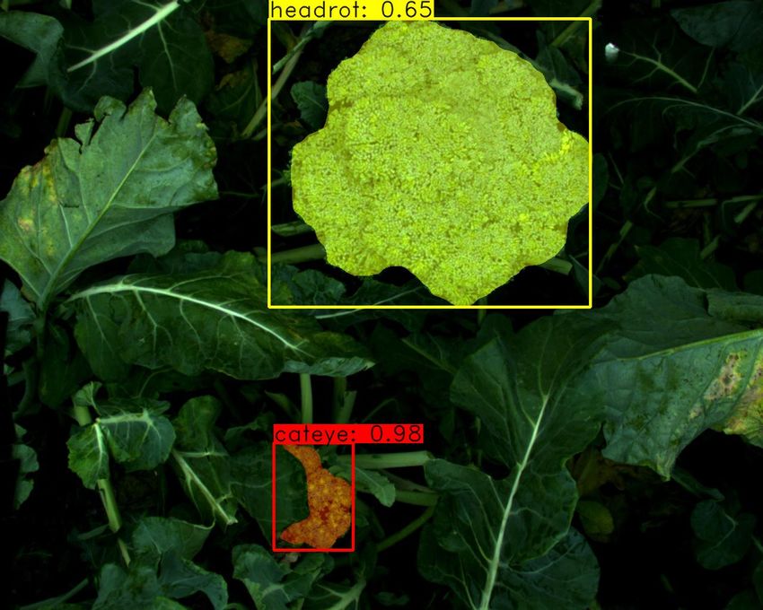
1    Introduction

Over the past decade, significant progress has been made in the research and development of deep learning
algorithms (LeCun et al., 2015). In particular, advances in convolutional neural networks (CNN) have led to
image analysis algorithms for autonomous cars, drones and robots (Pierson and Gashler, 2017; Sünderhauf
et al., 2018). One of the remaining challenges when optimising CNN’s for robot deployment, is that the CNN
must be able to work on new and untrained image scenes (Marcus, 2018; Mitchell, 2021). This is known as
generalisation (Goodfellow et al., 2016).

The key to generalisation is to train a CNN with enough images to cover the variation that exists in the
real world. Collecting a sufficient number of application-specific images can be challenging when the image
acquisition is difficult or expensive. For these situations, image synthesis techniques, such as generative
adversarial networks (GAN), have been proposed as a solution. With GAN’s, it is possible to create thousands
of synthetic images with a desired content from a small dataset of real images (Goodfellow et al., 2016). A
common limitation with image synthesis techniques, is that the synthetic images may not fully capture the
variance that exists in the real world (Rizvi et al., 2021).

Nowadays, in many cases, it is feasible to obtain large datasets of real images, due to the availability of
affordable camera systems and robot platforms. However, with the availability of large datasets, other
challenges occur, such as the selection and annotation of images to be used for training. Improper image
selection and annotation can lead to suboptimal performance. In addition, it is imperative to annotate only
the smallest possible number of images, when the image annotation can only be done by specialists with
specific knowledge about the image objects. Therefore, for large datasets with real images, it is important
to have a method that will maximise the CNN’s performance with as few image annotations as possible.

Active learning is a method that can achieve this goal (Ren et al., 2020). In active learning, the most
informative images are automatically selected from a large pool of unlabelled images. The most informative
images are then annotated manually or semi-automatically, and used for training the CNN. The hypothesis is
that the generalisation performance of the CNN significantly improves when the training is done on the most
informative images, because these are expected to have a higher information content for CNN optimisation
(Ren et al., 2020). Because only the most informative images need to be annotated with active learning, the
annotation effort will be reduced while maintaining or improving the performance of the CNN.

Much research has been done on active learning. The majority of the active learning methods were developed
for image classification, semantic segmentation, and object detection (Ren et al., 2020). For instance seg-
mentation, which is a combination of object detection and semantic segmentation, only three active learning
methods have been presented (López Gómez, 2019; Van Dijk, 2019; Wang et al., 2020). These three active
learning methods were all developed for the Mask Region-based CNN (Mask R-CNN) (He et al., 2017), and
all methods used uncertainty-based sampling. Uncertainty-based sampling selects the images about which
Mask R-CNN has the most uncertainty, with the idea that these will contribute most to improving Mask
R-CNN when it is retrained. The first active learning method for Mask R-CNN was developed by Van Dijk
(2019), and used the probabilistic active learning (PAL) method of Krempl et al. (2014). With PAL, the
expected performance gain was calculated for the unlabelled images, and the images with the highest gain
were selected for retraining. The second active learning method for Mask R-CNN was developed by Wang
et al. (2020), and used a learning loss method. With this method, three additional loss prediction modules
were added to the Mask R-CNN network to predict the loss of the class, box and mask of the unlabelled
images. Images with a high loss were selected and labelled in a semi-supervised way using the model’s
output. The third active learning method for Mask R-CNN was developed by López Gómez (2019). In this
work, the image sampling was done with Monte-Carlo dropout. Monte-Carlo dropout was introduced by
Gal and Ghahramani (2016) and it is a frequently used sampling technique in active learning, because of
its straightforward implementation. In this method, the image analysis is performed with dropout, causing
the random disconnection of some of the neurons of the CNN, which forces the CNN to make the decision
with another set of network weights. When the same image is analysed multiple times with dropout, the

                                                     4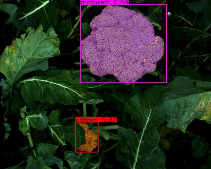
model output may differ between the different analyses. If the model output deviates, there seems to be
uncertainty about the image, indicating that it can be a candidate for selection and annotation.

In the work of López Gómez (2019), two uncertainty values were calculated: the semantic uncertainty
and the spatial uncertainty. The semantic uncertainty expressed the (in)consistency of Mask R-CNN to
predict the class labels on an instance. The spatial uncertainty expressed the (in)consistency of Mask
R-CNN to segment the object pixels of an instance. In the research of Morrison et al. (2019), an even
more comprehensive uncertainty calculation was proposed for Mask R-CNN. In this work, three uncertainty
values were calculated: the semantic uncertainty, the spatial uncertainty and the occurrence uncertainty.
The occurrence uncertainty expressed the (in)consistency of Mask R-CNN to predict instances on the same
object during the repeated image analysis. Morrison et al. (2019) showed an improved predictive uncertainty
of Mask R-CNN when combining the three uncertainty values into one hybrid value, compared to using the
three uncertainty values separately. Despite the promising results, the uncertainty calculation of Morrison
et al. (2019) has not yet been applied in an active learning framework.

Our study describes the research and development of a new active learning software framework, which was
based on the uncertainty calculation of Morrison et al. (2019). Our active learning framework was developed
for Mask R-CNN, and it was named MaskAL. We hypothesised that by using MaskAL, the performance
of Mask R-CNN can be improved faster and thereby the annotation effort can be reduced compared to a
random sampling method. Our research objective was to test this hypothesis on a large and diverse image
dataset of field-grown broccoli (Brassica oleracea var. italica).

The primary contribution of our work is a new active learning software framework for Mask R-CNN. Part
of our novelty is the updated semantic uncertainty calculation compared to Morrison et al. (2019). The
secondary contribution of our work is a quantitative analysis of the effects of four uncertainty calculation
parameters on the active learning performance.

                                                     5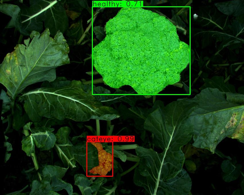
2       Materials and methods

This section is divided into three paragraphs. Paragraph 2.1 describes the image dataset that was used for
training and evaluation of MaskAL. Paragraph 2.2 describes the implementation of MaskAL. Paragraph 2.3
describes the experiments that were conducted to compare the performance between the active learning and
the random sampling.

2.1     Image dataset

2.1.1    Images

Our dataset consisted of 16,000 red, green, blue (RGB) colour images of field-grown broccoli. The images were
acquired on 26 commercial broccoli fields in seven growing seasons (2014-2021) in four countries (Australia,
the Netherlands, the United Kingdom (UK), and the United States of America (USA)). All images were
taken with a top-view camera perspective.

4622 of the 16,000 images were downloaded from three online available broccoli image datasets (Bender
et al., 2019; Blok et al., 2021b; Kusumam et al., 2016). The images in these datasets were acquired with a
Ladybird robot (Figure 1a), a stationary camera frame (Figure 1b) and a tractor-mounted acquisition box
(Figure 1c). The other 11,378 images were acquired with an image acquisition system that was attached to
a selective broccoli harvesting robot (Figure 1d) (Blok et al., 2021a). The detailed information about the
broccoli fields, crop conditions, and camera systems can be found in Table 1.

2.1.2    Annotation and class labels

In our research, every image was annotated, because this allowed us to conduct three experiments without
being interrupted for doing the image annotations. The image annotations were done by two crop experts,
who used the LabelMe software (version 4.5.6) (Wada, 2016) to annotate a total of 31,042 broccoli heads in
the 16,000 images. The experts assigned one of five potential classes to each broccoli head: healthy, damaged
(defect), matured (defect), cateye (defect), or headrot (disease). Examples of these five classes are visualised
in Figure 2. The choice of these five broccoli classes was based on the potential use of the Mask R-CNN
model on a selective broccoli harvesting robot. An adequately trained Mask R-CNN model will allow the
robot to determine, under all conditions, which broccoli heads are both healthy and large enough to be
harvested. Broccoli heads with defects or disease should be detected by Mask R-CNN so that the robot is
able to locate them in the field rather than harvest them.

2.1.3    Training pool, validation set and test set

Because the images were taken primarily on moving machines, it could happen that a unique broccoli head
was photographed several times. To avoid the training, validation, or test set containing images of the
same broccoli head, we first grouped the image frames of unique broccoli heads. This grouping was possible
because each image had a real world coordinate assigned by the global navigation satellite system (GNSS)
that was installed on the image acquisition device. With the real world coordinates, it was possible to
uniquely identify the broccoli heads according to their position and to group the image frames belonging to
the same broccoli head. After grouping, the image frames belonging to a unique broccoli head were placed
into either the training pool, validation set, or test set.

The training pool consisted of 14,000 images, and these images could be used to train Mask R-CNN and
to sample new images. In the training pool, there was a high class imbalance (Figure 3a), because in field
conditions there is a higher chance of photographing a healthy broccoli head than photographing a broccoli
head with a defect or disease.

                                                       6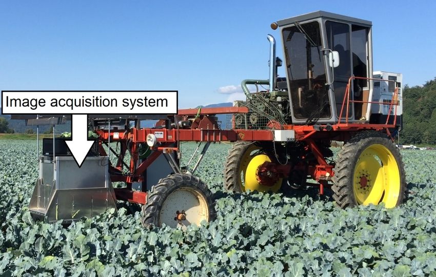
(a)                                                           (b)

                        (c)                                                           (d)

Figure 1: Overview of the image acquisition systems that were used to acquire the broccoli dataset. (a) With
the Ladybird robot, broccoli images were acquired in Cobbitty (Australia) in 2017. The displayed image is
from Bender et al. (2020). (b) With a stationary camera setup, broccoli images were acquired in Sexbierum
(the Netherlands) in 2020. The displayed image is from Blok et al. (2021c). (c) With a tractor-mounted
acquisition box, broccoli images were acquired in Surfleet (the United Kingdom) in 2015. The displayed
image is from Kusumam et al. (2017). (d) With a selective broccoli harvesting robot, broccoli images were
acquired in the Netherlands and the United States of America in the period 2014-2021. The displayed image
is from Blok et al. (2021c).

The validation set consisted of 500 images. These validation images were used during the training process to
check whether Mask R-CNN was overfitting. The validation images were selected with a stratified sampling
criterion based on the information of the broccoli field and the class label of the annotation. This stratified
sampling ensured that the images of each field would end up in the validation set, and that there would be
a rather balanced ratio of the five classes in the validation set, see Figure 3b.

Instead of one test set, we used three test sets of 500 images each. The three test sets were completely
independent of the training process. Each test set served as an independent image set for each of our three
experiments (refer to paragraph 2.3). Because the outcome of an experiment influenced the parameter choice
in the next experiment, new test sets were needed that were independent of the previously used test set.
The image selection of the three test sets was based on the same stratified sampling criterion that was used
for the validation set. As a result, the three test sets had a rather balanced ratio of the five classes to better
test the Mask R-CNN performance on the five broccoli classes (refer to Figures 3c, 3d, and 3e).

                                                        7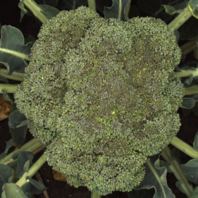
Table 1: The 16,000 broccoli images were acquired on 26 fields in four countries: Australia (AUS), The
Netherlands (NL), United Kingdom (UK) and United States of America (USA). The column ”Acq. days”
lists the number of image acquisition days performed on that particular field. The column ”Ref.” refers to
the reference of the publicly available image dataset.

 Field     Year    Country          Place            Total      Acq.       Broccoli       Camera Ref.
                                                    images      days       cultivar
 1         2014     NL          Oosterbierum         1105         2         Steel           1
 2         2015     NL          Oosterbierum          286         3       Ironman           1
 3         2015     NL           Sexbierum            480         3         Steel           1
 4         2015     UK             Surfleet          2122         1       Ironman           2        A
 5         2016     NL           Sexbierum            270         2       Ironman           1
 6         2016     NL          Oosterbierum          206         1         Steel           1
 7         2016     NL           Sexbierum            415         3         Steel           1
 8         2016     NL           Sexbierum            646         2         Steel           1
 9         2016     NL           Sexbierum            168         1         Steel           1
 10        2017     AUS           Cobbitty            915         2       Unknown           3        B
 11        2017     NL           Sexbierum            256         4       Ironman           1
 12        2017     NL          Oosterbierum          481         2       Ironman           1
 13        2017     NL          Oude Bildtzijl        149         1       Unknown           1
 14        2018     USA       Santa Maria (CA)       2180        11        Avenger          4
 15        2018     USA       Burlington (WA)        1977         8     Emerald Crown       4
 16        2018     USA       Burlington (WA)         385         3     Emerald Crown       4
 17        2019     USA       Santa Maria (CA)         85         3         Eiffel          5
 18        2019     USA        Guadalupe (CA)         233         5        Avenger         4&5
 19        2019     USA      Mount Vernon (WA)        660         2      Green Magic        4
 20        2019     USA      Mount Vernon (WA)        619         1      Green Magic        4
 21        2020     USA       Burlington (WA)         120         1     Emerald Crown       4
 22        2020     NL           Sexbierum            565         1       Ironman           5        C
 23        2020     NL           Sexbierum           1020         1       Ironman           5        C
 24        2021     USA         Blythe (CA)           344         1       Unknown           6
 25        2021     USA       Santa Maria (CA)        119         1         Eiffel          6
 26        2021     USA       Basin City (WA)         194         1      Green Magic        6
Camera 1: AVT Prosilica GC2450, Camera 2: Microsoft Kinect 2, Camera 3: Point Gray GS3-U3-120S6C-C,
Camera 4: IDS UI-5280FA-C-HQ, Camera 5: Intel Realsense D435, Camera 6: Framos D435e
Reference A: Kusumam et al. (2016), Reference B: Bender et al. (2019), Reference C: Blok et al. (2021b)

                                                    8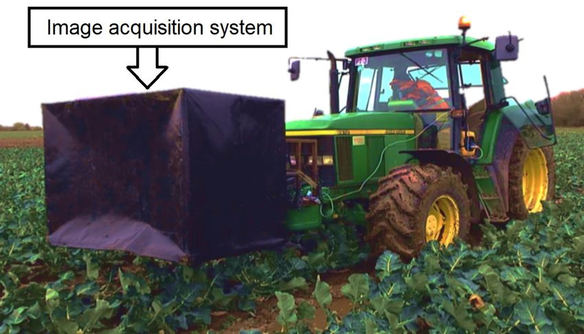
(a)                   (b)                   (c)                   (d)                   (e)

Figure 2: Examples of the five broccoli classes that were annotated in our dataset: (a) An example of a
healthy broccoli head that should be harvested by the robot. (b) A damaged broccoli head that should not
be harvested by the robot. Broccoli heads can be damaged when they are hit by the machinery or human
harvesters. (c) A matured broccoli head that should not be harvested, because the florets started to bloom.
(d) A cateye broccoli head that should not be harvested, because some florets turned yellow. (e) A headrot
broccoli head that should not be harvested, because the florets started to rot. The displayed images were
all cropped from a bigger field image.

                  (a)                                      (b)                                  (c)

                                 (d)                                     (e)

Figure 3: Distribution of the classes that were annotated: (a) training pool (b) validation set (c) test set 1
(d) test set 2 (e) test set 3.

                                                      9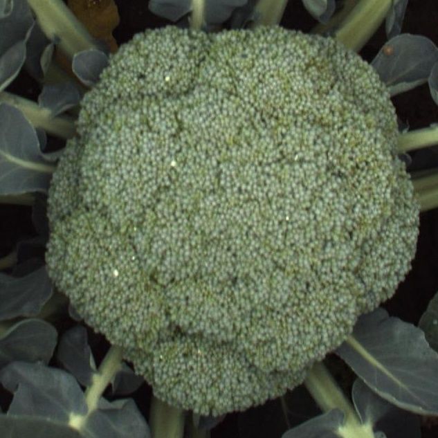
2.2     MaskAL

Paragraph 2.2.1 describes the implementation details of the MaskAL software. The neural network archi-
tecture is described in paragraph 2.2.2. Paragraph 2.2.3 and 2.2.4 describe the training and evaluation
procedures. In paragraph 2.2.5, the uncertainty-based sampling method of MaskAL is described.

2.2.1    MaskAL software

The MaskAL software was based on the Mask R-CNN software of Detectron2 (version 0.4) (Wu et al., 2019).
The pseudo-code of MaskAL can be found in Algorithm 1. The software began by creating an initial dataset,
which was randomly sampled from the training pool (line 3 of Algorithm 1). After the image annotation (line
4 of Algorithm 1), Mask R-CNN was trained using the weights of a Mask R-CNN model that was pretrained
on the Microsoft Common Objects in Context (COCO) dataset (Lin et al., 2014) (see line 5 of Algorithm 1).
The network weights with the highest performance on the validation dataset were automatically selected,
and these weights were used to evaluate the images of the independent test set (line 6 of Algorithm 1). The
performance metric was the mean average precision (mAP), which expressed the classification and instance
segmentation performance of Mask R-CNN. A mAP value close to zero indicated an incorrect classification
and/or inaccurate instance segmentation, while a value close to 100 indicated a correct classification and
accurate instance segmentation.

After the evaluation, the available images for sampling were obtained by removing the training images from
the training pool (line 8 of Algorithm 1). The sampling of new images was done with one of two available
sampling methods: uncertainty sampling (active learning) and random sampling. The uncertainty sampling
used the trained Mask R-CNN model to sample the images about which the model had the most uncertainty
(line 11 of Algorithm 1). The uncertainty sampling is explained in more detail in paragraph 2.2.5. The
random sampling did not use the trained model but a random sample method to select the images (line 13
of Algorithm 1).

After sampling, the selected images were annotated (line 14 of Algorithm 1). The new set of annotated
images was added to the previous set of training images (line 15 of Algorithm 1). Mask R-CNN was trained
on this combined image set, using the weights of the previously trained Mask R-CNN model (lines 16 and
17 of Algorithm 1). This transfer learning method allowed faster optimisation of the network weights. The
network weights with the highest performance on the validation dataset were used to evaluate the images of
the independent test set (line 18 of Algorithm 1). After this evaluation, the available images for sampling
were updated by removing the training images from the training pool (line 20 of Algorithm 1). The entire
procedure was repeated until a user-specified number of sampling iterations was reached (line 9 of Algorithm
1).

2.2.2    Network architecture

Before the training and sampling could be performed, dropout had to be applied to several network layers of
Mask R-CNN. In the box head of Mask R-CNN, dropout was applied to each fully connected layer, see Figure
4. This dropout placement was in line with Gal and Ghahramani (2016) and would allow us to capture the
variation in the predicted classes and the bounding box locations. Additionally, we chose to apply dropout
to the last two convolutional layers in the mask head of Mask R-CNN to be able to capture the variation in
the pixel segmentation, see Figure 4.

The severity of the dropout was made configurable in the software by means of the dropout probability.
The dropout probability determined the chance of neurons getting disconnected in a network layer. The
probability could be configured between 0.0 (no dropout) and 1.0 (complete dropout). The backbone of
Mask R-CNN was ResNeXt-101 (32x8d) (Xie et al., 2017), which was chosen because it was the best feature
extractor available in the Detectron2 software.

                                                    10
Algorithm 1: MaskAL
Inputs : sampling-method : ’uncertainty’ or ’random’
sampling-iterations : integer
sample-size : integer
initial-dataset-size : integer
dropout-probability: float
forward-passes : integer
certainty-method : ’average’ or ’ minimum’
training-pool : dataset with all available images for training and sampling
val-set : validation dataset
test-set : test dataset
Outputs: mAPs : an array with mean average precision values of size sampling-iterations+1
1 Function MaskAL(sampling-method, sampling-iterations, sample-size, initial-dataset-size,
dropout-probability, forward-passes, certainty-method, training-pool, val-set, test-set):
2 mAPs ← [ ]
3 initial-dataset ← SampleInitialDatasetRandomly(training-pool, initial-dataset-size)
4 annotated-train-set, annotated-val-set, annotated-test-set ← Annotate(initial-dataset, val-set, test-set)
5 model ← TrainMaskRCNN(annotated-train-set, annotated-val-set, coco-weights, dropout-probability)
6 mAP ← EvalMaskRCNN(model, annotated-test-set)
7 mAPs.insert(mAP)
8 available-images ← training-pool − initial-dataset
9 for i ← 1 to sampling-iterations do
10 if sampling-method = ’uncertainty’ then
11 pool ← UncertaintySampling(model, available-images, sample-size, dropout-probability,
forward-passes, certainty-method)
12 else if sampling-method = ’random’ then
13 pool ← RandomSampling(available-images, sample-size)
14 annotated-pool ← Annotate(pool)
15 annotated-train-set ← annotated-train-set + annotated-pool
16 prev-weights ← model
17 model ← TrainMaskRCNN(annotated-train-set, annotated-val-set, prev-weights, dropout-probability)
18 mAP ← EvalMaskRCNN(model, annotated-test-set)
19 mAPs.insert(mAP)
20 available-images ← available-images − annotated-pool
21 end
22 return mAPs
11Figure 4: Schematic representation of the Mask R-CNN network architecture in MaskAL. The white circles
with the red crosses indicate the network layers with dropout. Conv., DO, RPN, ROI and FC, are abbrevia-
tions of respectively convolutional, dropout, region proposal network, region of interest, and fully connected
layers. The numbers between brackets give the output dimensions of the ROIAlign layer. The image was
adapted from Shi et al. (2019).
2.2.3 Training
The training procedure of Mask R-CNN was identical for the active learning and the random sampling. The
training was performed with dropout as a regularisation technique to enhance the generalisation performance
(refer to lines 5 and 17 of Algorithm 1). This procedure was in line with the training procedure of Gal and
Ghahramani (2016). The stochastic gradient descent optimiser was used with a momentum of 0.9 and
a weight decay of 1.0·10-4 . Two data augmentations were used during training to further enhance the
generalisation performance. The first data augmentation was a random horizontal flip of the image with
a probability of 0.5. The second data augmentation was an image resizing along the shortest edge of the
image while maintaining the aspect ratio of the image. The image batch size was two and the learning rate
was 1.0·10-2 . The total number of training iterations was proportional to the number of training images. As
such, a more extensive training was performed when there were more images, see Table 2.
Table 2: The number of Mask R-CNN training iterations was proportional to the number of training images.
Number of Number of Mask R-CNN
training images training iterations
1 - 500 2.500
501 - 1000 5.000
1001 - 1500 7.500
1501 - 2000 10.000
2001 - 2500 12.500
... ...
13.501 - 14.000 70.000
In our training pool, there was a severe class imbalance (see Figure 3a). Due to this class imbalance, the
random sampling was more likely to sample images with healthy broccoli heads than images with damaged,
matured, cateye or headrot broccoli heads. This could eventually lead to a much worse performance than
the active learning. To prevent that our comparison would be too much influenced by the class imbalance,
it was decided to train Mask R-CNN with a data oversampling strategy (Gupta et al., 2019). With this
strategy, a specific image was repeatedly trained by Mask R-CNN if that image contained a minority class
(the minority classes were damaged, matured, cateye and headrot). By repeating the images with minority
12classes during the training, this oversampling strategy was expected to reduce the negative effect of the class
imbalance on the Mask R-CNN performance.
2.2.4 Evaluation
After the training, the mAP value was obtained on the images of the test set. This evaluation was done
without dropout, and with a fixed threshold of 0.01 on the non-maximum suppression (NMS). This NMS
threshold removed all instances that overlapped at least 1% with a more confident instance, essentially
meaning that only one instance segmentation was done on an object. This approach was considered valid
since the broccoli heads grew solitary and did not overlap each other in the images.
2.2.5 Uncertainty sampling
After the training and evaluation, the trained Mask R-CNN model was used to sample images from the
training pool about which the model had the most uncertainty. The uncertainty sampling is explained in
Algorithm 2, and it involved four steps: the repeated image analysis with Monte-Carlo dropout (paragraph
2.2.5.1), the grouping of the instance segmentations into instance sets (paragraph 2.2.5.2), the calculation of
the certainty values (paragraph 2.2.5.3) and the sampling of the images (paragraph 2.2.5.4).
Algorithm 2: UncertaintySampling
Inputs : model : trained Mask R-CNN model
available-images : dataset with all available images for sampling
sample-size : integer
dropout-probability: float
forward-passes : integer
certainty-method : ’average’ or ’ minimum’
Outputs: pool : set of images about which Mask R-CNN had the most uncertainty
1 Function UncertaintySampling(model, available-images, sample-size, dropout-probability,
forward-passes, certainty-method):
2 certainty-values ← [ ]
3 for i ← 0 to length(available-images) − 1 do
4 image ← available-images[i]
5 predictions ← MonteCarloDropout(model, image, dropout-probability, forward-passes)
6 instance-sets ← CreateInstanceSets(predictions)
7 certainty-value ← CalculateCertaintyValue(instance-sets, certainty-method)
8 certainty-values.insert(certainty-value, image)
9 end
10 pool ← GetMostUncertainImages(certainty-values, sample-size)
11 return pool
2.2.5.1 Monte-Carlo dropout method
Each available image from the training pool was analysed with the trained Mask R-CNN model in the Monte-
Carlo dropout method. A user-specified number of forward passes determined how many times the same
image was analysed with the trained Mask R-CNN model (line 5 of Algorithm 2). During the repeated image
analysis, the dropout caused the random disconnection of some of the neurons in the head branches of Mask
R-CNN. This random neuron disconnection could lead to different model outputs, see Figure 5a, 5b and 5c.
The repeated image analysis was done with a fixed threshold of 0.01 on the non-maximum suppression and
a fixed threshold of 0.5 on the confidence level.
13(a) (b)
(c) (d)
Figure 5: A visual example of the Monte-Carlo dropout method and the calculation of the certainty values.
(a) After the first forward pass with dropout, Mask R-CNN produced two instances: one instance of class
cateye with a high confidence score (0.98) and one instance of class headrot with a lower confidence score
(0.65). (b) The same image was analysed again during a second forward pass, resulting a confident cateye
instance (0.97) and a less confident matured instance (0.59). (c) After the third forward pass, Mask R-CNN
produced a confident cateye instance (0.99) and a moderately confident healthy instance (0.71). (d) After
the three forward passes, the instances were grouped into two instance sets, based on spatial similarity. An
instance set is a group of different instance segmentations that appear on the same broccoli head. The white
bounding box and mask of the instance sets represent the average box and mask of the corresponding three
predicted instance segmentations. On each instance set, three certainty values were calculated: the semantic
certainty (csem ), the occurrence certainty (cocc ) and the spatial certainty (cspl ), which was the product of the
spatial certainty of the bounding box (cbox ) and the mask (cmask ). The certainty of the instance set (ch ) was
calculated by multiplying the csem , cocc and cspl .
2.2.5.2 Instance sets
After the repeated image analysis, the outputs of Mask R-CNN were grouped into instance sets (line 6 of
Algorithm 2). An instance set is a group of different instance segmentations from multiple forward passes
14that appear on the same object in the image, see two examples in Figure 5d. On these instance sets, the
certainty values were calculated.
The grouping of the segmentations into instance sets was based on spatial similarity, a method that was
introduced by Morrison et al. (2019) for instance segmentation. The grouping method added an instance
segmentation to an instance set when the intersection over union (IoU) between this segmentation and at
least one other segmentation from the instance set exceeded a certain threshold, τIoU . The IoU is a metric
for the spatial overlap between two mask segmentations, M1 and M2 , and the value varies between zero (no
overlap) and one (complete overlap), see Equation 1.
|M1 ∩ M2 |
IoU(M1 , M2 ) = where | · | gives the total number of mask pixels (1)
|M1 ∪ M2 |
A new instance set was created when the segmentation did not exceed the τIoU threshold. It was assumed
that this segmentation then represented a different object. In our research, the τIoU was set to 0.5 and this
value was adopted from Morrison et al. (2019).
2.2.5.3 Certainty calculation
Three certainty values were calculated for each instance set: the semantic certainty, the spatial certainty,
and the occurrence certainty. The certainty calculation methods were adopted from Morrison et al. (2019),
but changes were made to the semantic certainty calculation.
The semantic certainty, csem , was a measure of the consistency of Mask R-CNN to predict the class labels
within an instance set. The csem value was close to zero when there was a low semantic certainty, and close to
one when there was a high semantic certainty. Morrison et al. (2019) calculated the csem value by taking the
difference between the average confidence score of the first and the second most probable class of the instance
set. This method is known as margin sampling, but a disadvantage is that it does not take into account
the confidence scores of the less probable classes. This is undesirable when the dataset has a high degree of
inter-class similarity, because then Mask R-CNN has a tendency to hesitate between more than two classes.
This multi-class hesitation was also expected in our dataset, because the broccoli classes were visually similar
(Figure 2). To overcome the disadvantage of the margin sampling, the csem calculation was upgraded with an
entropy-based equation, which took the confidence scores, P , of all classes, K = {k1 , . . . , kn }, into account,
see Equation 2. However, with the entropy calculation, the csem value would be low when there was class
certainty, and this was opposite of Morrison’s csem value. Also, the entropy calculation could result in values
higher than one, which deviated from Morrison’s csem value that was bound between zero and one. With two
additional calculations these issues were solved. First, the entropy value, H, was divided by the maximum
entropy value, Hmax , so that the resulting value was bound between zero and one (see Equation 3). The Hmax
value was calculated with Equation 4, and this value represented a situation where the confidence scores of
all classes were equal, which was the case when Mask R-CNN had the lowest certainty in predicting the class
labels. Then, the resulting value from the division was inverted, such that a high Hsem value would result
when there was a high semantic certainty. With Equation 5, the Hsem values of all instances belonging to
an instance set, S = {s1 , . . . , sn }, were averaged. This resulted in one semantic certainty value, csem , per
instance set. Figure 5d visualises two estimations of csem .
n
X
H(K) = − P (ki ) · log P (ki ) with K = {k1 , . . . , kn } (2)
i=1
H(K)
Hsem (s) = 1 − where s is an instance of instance set S (3)
Hmax (K)
151
· log n1
Hmax (K) = −n · n where n is the number of classes (4)
n
1 X
csem (S) = · Hsem (si ) with S = {s1 , . . . , sn } (5)
n i=1
The spatial certainty, cspl , was a measure of the consistency of Mask R-CNN to determine the bounding box
locations and to segment the object pixels within an instance set. The cspl value was close to zero when there
was little spatial consistency between the boxes and the masks in the instance set, and the value was close
to one when there was much spatial consistency. The cspl value was calculated by multiplying the spatial
certainty value of the bounding box (cbox ) by the spatial certainty value of the mask (cmask ), see Equation 6.
The cbox and the cmask values were the mean IoU values between the average box and mask of the instance
set (respectively denoted as B̄ and M̄ ) and each individual box and mask prediction within that instance
set (respectively denoted as B and M ), refer to Equation 7 and 8. The average box, B̄, was formed from
the centroids of the corner points of the individual boxes in the instance set (see the white boxes in Figure
5d). The average mask, M̄ , represented the segmented pixels that appeared in at least 25% of the individual
masks in the instance set (see the white masks in Figure 5d). The value of 25% was found to produce the
most consistent average masks for our broccoli dataset.
cspl (S) = cbox (S) · cmask (S) with S = {s1 , . . . , sn } (6)
n
1 X
cbox (S) = · IoU(B̄(S), B(si )) with S = {s1 , . . . , sn } (7)
n i=1
n
1 X
cmask (S) = · IoU(M̄ (S), M (si )) with S = {s1 , . . . , sn } (8)
n i=1
The occurrence certainty, cocc , was a measure of the consistency of Mask R-CNN to predict instances on
the same object during the repeated image analysis. The cocc value was close to zero, when there was little
consensus in predicting an instance on the same object in each forward pass. The cocc value was one when
Mask R-CNN predicted an instance on the same object in each forward pass. The cocc value was calculated
by dividing the number of instances belonging to an instance set, n, by the number of forward passes, f p,
see Equation 9.
n
cocc (S) = with S = {s1 , . . . , sn } (9)
fp
The semantic, spatial, and occurrence certainty values were multiplied into one certainty value for each
instance set, see Equation 10. With this multiplication, the three certainty values were considered equally
important in determining the overall certainty, ch , of an instance set.
ch (S) = csem (S) · cspl (S) · cocc (S) with S = {s1 , . . . , sn } (10)
Because the Mask R-CNN training and testing was done on images and not on individual instances, it was
needed to combine the certainties of the instance sets into one certainty value for the entire image. The
image certainty value was calculated with either the average method or the minimum method. With the
16average method, the image certainty value was the average certainty value of all instance sets in the image,
I = {S1 , . . . , Sn }, see Equation 11. In Figure 5d, the average certainty value was 0.62 ((0.88 + 0.37)/2).
With the minimum method, the image certainty value was the lowest certainty value of all instance sets,
see Equation 12. In Figure 5d, the minimum certainty value was 0.37. The certainty calculation method
was made configurable in the software (see line 7 of Algorithm 2), so that we could do an experiment to
assess the effect of the certainty calculation method on the active learning performance (this is explained in
paragraph 2.3.1).
n
1 X
cavg (I) = · ch (Si ) with I = {S1 , . . . , Sn } (11)
n i=1
cmin (I) = min(ch (I)) with I = {S1 , . . . , Sn } (12)
2.2.5.4 Sampling
After calculating the certainty value of each image from the training pool, a set of images was selected about
which Mask R-CNN had the most uncertainty. These images were annotated and used to retrain Mask
R-CNN. The size of the image set, hereinafter referred to as the sample size, was made configurable in the
software (line 10 of Algorithm 2). This allowed us to do an experiment to assess the effect of the sample size
on the active learning performance (this is explained in paragraph 2.3.2).
2.3 Experiments
Three experiments were set up, with the final objective of comparing the performance of the active learning
with the performance of the random sampling. Before this comparison could be done, experiments 1 and 2
were performed to investigate how to optimise the active learning.
2.3.1 Experiment 1
The objective of experiment 1 was to test the effect of the dropout probability, certainty calculation method,
and number of forward passes on the active learning performance. This test would reveal the optimal settings
for these parameters, which were assumed to have the most influence on the active learning performance,
because they all influenced the calculation of the certainty value of the image.
The experiment was done with three dropout probabilities: 0.25, 0.50, and 0.75. Dropout probability 0.50
was a frequently used probability in analogous active learning research, for example Aghdam et al. (2019),
Gal and Ghahramani (2016) and López Gómez (2019). With this dropout probability, there was a moderate
chance of dropout during the image analysis. The dropout probabilities 0.25 and 0.75 were chosen to have
a lower chance of dropout and a higher chance of dropout, compared to the dropout probability 0.50.
Two certainty calculation methods were tested: the average method and the minimum method, which are
both described in paragraph 2.2.5.3. By comparing these two calculation methods, it was possible to evaluate
whether the active learning benefited from sampling the most uncertain instances (when using the minimum
method), or from sampling the most uncertain images (when using the average method).
Before we could evaluate the effect of the number of forward passes on the active learning performance, a
preliminary experiment was performed to examine which numbers were plausible in terms of consistency of
the certainty estimate. This consistency was considered important, because when the estimate is consistently
uncertain, there is more chance that the image actually contributes to the active learning performance. The
17setup and results of the preliminary experiment are described in Appendix A. Based on the results in
Appendix A, two numbers of forward passes were chosen: 20 and 40.
The three dropout probabilities, two certainty calculation methods, and two numbers of forward passes were
combined into 12 unique combinations of certainty calculation parameters. We assessed the effect of each
of these 12 combinations on the active learning performance. All combinations were tested with the same
initial dataset of 100 images, which were randomly sampled from the training pool. After training Mask
R-CNN on the initial dataset, the trained model was used to select 200 images from the remaining training
pool about which Mask R-CNN had the most uncertainty. The selected images were used together with the
initial training images to retrain Mask R-CNN. This procedure was repeated 12 times, such that in total
13 image sets were trained (containing respectively, 100, 300, 500, ..., 2500 sampled images). After training
Mask R-CNN on each image set, the performance of the trained model was determined on the images of the
first test set. The 13 resulting mAP values were stored. The experiment was repeated five times to account
for the randomised initial dataset and the randomness in the Monte-Carlo dropout method.
A three-way analysis of variance (ANOVA) with a significance level of 5% was employed for the 13 mAP
values to test whether there were significant performance differences between the three dropout probabilities,
the two certainty calculation methods, and the two numbers of forward passes. The ANOVA was performed
per mAP value, because the mAP was not independent between the different image sets (for instance, the
set of 2500 images contained the 2300 images from the previous sampling iteration).
2.3.2 Experiment 2
The optimal setting for the dropout probability, certainty calculation method, and number of forward passes
was obtained from experiment 1 and used in experiments 2 and 3. The objective of experiment 2 was to test
the effect of the sample size on the active learning performance. This experiment would reveal the optimal
sample size for annotating the images and retraining Mask R-CNN. A smaller sample size would possibly be
better for the active learning performance, because Mask R-CNN would then have more chances to retrain
on the images it was uncertain about. A larger sample size will reduce the total sampling time.
Four sample sizes were tested: 50, 100, 200, and 400 images. These four sample sizes were considered the
most practical in terms of annotation and retraining time. For all sample sizes, the initial dataset size was
100 images and the maximum number of training images was 2500 images. Both numbers were considered
realistic for datasets like ours, with less than five objects per image. The number of sampling iterations for
the four sample sizes was respectively, 48, 24, 12, and 6. The performances of the trained Mask R-CNN
models were determined on the images of the second test set. The experiment was repeated five times to
account for the randomised initial dataset and the randomness in the Monte-Carlo dropout method.
A one-way ANOVA with a significance level of 5% was employed for the mAP values to test whether there
were significant performance differences between the four sample sizes. The ANOVA was performed on the
mAP values that shared a common number of training images (the common numbers were 500, 900, 1300,
1700, 2100, and 2500 images). The ANOVA was not performed on the mAP value of the initial dataset,
because this value was identical between the four sample sizes (this was because the Mask R-CNN training
was performed with the same dropout probability).
2.3.3 Experiment 3
The objective of experiment 3 was to compare the performance of the active learning with the performance of
the random sampling. With random sampling, Mask R-CNN was trained with the same dropout probability
that was chosen from experiment 1. The initial dataset size was 100 images, and both sampling methods used
the same sample size that was chosen from experiment 2. The performances of the trained Mask R-CNN
models were determined on the images of the third test set. The experiment was repeated five times to
account for the randomised initial dataset and the randomness in the Monte-Carlo dropout method. A one-
18way ANOVA with a significance level of 5% was employed to test whether there were significant performance
differences between the active learning and the random sampling. The ANOVA was not performed on the
mAP value of the initial dataset, because this value was identical between the two sampling methods (since
the training was performed with the same dropout probability).
For comparison, another Mask R-CNN model was trained on the entire training pool (14,000 images). This
model was trained until 70,000 training iterations were reached (Table 2). The performance of this model
was also evaluated on the images of the third test set. The resulting mAP value was considered as the
maximum mAP that could have been reached on our dataset.
193 Results
The results are summarised per experiment: experiment 1 (paragraph 3.1), experiment 2 (paragraph 3.2),
and experiment 3 (paragraph 3.3).
3.1 The effect of the dropout probability, certainty calculation method, and number of
forward passes on the active learning performance (experiment 1)
In Table 3, the ANOVA’s pairwise test is summarised for the three dropout probabilities, the two numbers
of forward passes, the two certainty calculation methods, and the thirteen sampling iterations. The dropout
probability had the largest effect on the active learning performance. For all but one sampling iteration,
the dropout probability 0.75 had a significantly lower mAP than the dropout probabilities 0.25 and 0.50.
The mAP difference was maximally 20.1 (between the dropout probabilities 0.25 and 0.75 at the third
sampling iteration). In five sampling iterations (1, 2, 3, 11, and 12), the dropout probability 0.25 had
a significantly higher mAP than the dropout probability 0.50. These results were in line with Figure 9
(Appendix A), which showed that the dropout probability 0.25 had the most consistent certainty estimate.
Dropout probability 0.25 was chosen as the preferred probability for the next experiments. This decision
meant that five significant interactions between the dropout probability and the certainty calculation method
were ignored (these interactions were all due to the dropout probability 0.75). There were no significant
interactions between the dropout probability and the number of forward passes.
Between the two numbers of forward passes, three significant differences were found at sampling iterations
8, 11, and 12. In these sampling iterations, the mAP was significantly higher at 20 forward passes. This
outcome was unexpected, as Figure 9 (Appendix A) showed that there was a less consistent certainty estimate
at 20 forward passes than at 40 forward passes. It should be noted that the mAP differences between 20
and 40 forward passes were relatively small (maximally 1.7 mAP). Furthermore, the significant difference in
sampling iteration 11 was entirely due to the dropout probabilities 0.50 and 0.75. Based on this outcome,
we decided to choose 20 forward passes in the next experiments. One significant interaction between the
number of forward passes and the certainty calculation method was ignored.
The performance differences between the two certainty calculation methods were small (maximally 1.3 mAP).
In one sampling iteration (10), the average method had a significantly higher mAP than the minimum
method. This significant difference was entirely due to the dropout probability 0.75. The small mAP
differences were probably due to the limited number of broccoli instances per image. There were on average
two broccoli instances per image, suggesting that the choice of the average or the minimum method probably
did not have much influence on the active learning performance. Despite the small mAP differences, we
decided to choose the average method in the next experiments.
20Table 3: Performance means expressed for the three dropout probabilities, the two numbers of forward
passes, the two certainty calculation methods, and the thirteen sampling iterations. Performance means
with a different letter are significantly different at a significance level of 5% (p=0.05).
Number of Performance (mAP)
Sampling training Dropout probability Forward passes Certainty method
iteration images 0.25 0.50 0.75 20 40 average minimum
1 100 21.5 a 18.4 b 12.4 c 17.4 a 17.5 a 17.2 a 17.7 a
2 300 35.8 a 31.3 b 17.5 c 28.6 a 27.8 a 27.7 a 28.8 a
3 500 42.1 a 37.5 b 22.0 c 34.1 a 33.6 a 33.5 a 34.3 a
4 700 47.9 a 46.1 a 31.5 b 41.7 a 41.9 a 41.4 a 42.2 a
5 900 49.8 a 49.6 a 36.3 b 45.3 a 45.1 a 45.0 a 45.5 a
6 1100 53.1 a 52.7 a 41.0 b 49.3 a 48.6 a 48.9 a 49.0 a
7 1300 54.5 a 53.2 a 46.0 b 51.7 a 50.8 a 51.5 a 51.0 a
8 1500 56.5 a 55.3 a 49.7 b 54.7 a 53.0 b 53.8 a 53.9 a
9 1700 57.2 a 57.5 a 54.0 b 56.8 a 55.7 a 56.8 a 55.6 a
10 1900 59.0 a 58.2 a 55.5 b 58.0 a 57.2 a 58.2 a 56.9 b
11 2100 60.1 a 58.4 b 56.9 c 59.1 a 57.8 b 58.6 a 58.3 a
12 2300 60.6 a 58.7 b 57.8 b 59.7 a 58.4 b 59.2 a 58.9 a
13 2500 61.1 a 60.2 a 58.6 b 60.4 a 59.5 a 60.2 a 59.7 a
3.2 The effect of the sample size on the active learning performance (experiment 2)
In Table 4, the ANOVA’s pairwise test is summarised for the four sample sizes and the seven sampling
iterations. Sample size 200 had the significantly highest mAP for all sampling iterations. In sampling
iteration 2, sample size 200 had a significantly higher mAP than sample size 400. The mAP difference was
5.5. An explanation for this difference is that with sample size 200, there was one additional retraining of
Mask R-CNN compared to sample size 400. In sampling iteration 3, sample size 200 had a significantly
higher mAP than sample size 50. In the four other sampling iterations, both sample sizes 200 and 400 had a
significantly higher mAP than sample sizes 50 and 100. This result was unexpected, as it was believed that
a smaller sample size could achieve better active learning performance, because Mask R-CNN would then
have more chances to improve itself on images about which the model was uncertain.
An in-depth analysis indicated that the performance gains of sample sizes 200 and 400 were mainly due to
a higher performance on the minority classes cateye and headrot. Figures 6c and 6d show that sample sizes
200 and 400 sampled a higher percentage of these classes compared to sample sizes 50 and 100 (Figures 6a
and 6b). Apparently, for the active learning performance, it was better to sample with larger image batches
that primarily consisted of one or two minority classes, than to sample with smaller image batches that had
a more balanced ratio of the minority classes.
One research demarcation may have influenced the results. In experiment 1, only sample size 200 was tested,
and this may have resulted that the chosen parameters from experiment 1 were only optimised for sample
size 200 and not for sample sizes 50, 100 and 400. Despite this research demarcation, we decided to choose
sample size 200 in the next experiment.
21Table 4: Performance means for the four sample sizes and the seven sampling iterations that shared a
common number of training images. Performance means with a different letter are significantly different at
a significance level of 5% (p=0.05). The ANOVA was not performed on the mAP value of the initial dataset
(100 images).
Performance (mAP)
Sampling Number of Sample size
iteration training images 50 100 200 400
1 100 22.4 - 22.4 - 22.4 - 22.4 -
2 500 40.9 a 41.6 a 42.2 a 36.7 b
3 900 47.5 b 48.8 ab 50.5 a 48.4 ab
4 1300 51.0 b 50.3 b 55.2 a 55.6 a
5 1700 53.1 b 51.7 b 57.9 a 57.5 a
6 2100 54.3 b 56.1 b 58.9 a 60.2 a
7 2500 56.7 c 57.3 bc 59.5 ab 60.5 a
(a) (b)
(c) (d)
Figure 6: Cumulative percentages of the sampled classes in experiment 2 (y-axis). The percentages are
expressed for the seven numbers of training images (x-axis) that were shared between the four sample sizes:
(a) sample size 50 (b) sample size 100 (c) sample size 200 (d) sample size 400.
223.3 Performance comparison between active learning and random sampling (experiment 3)
Figure 7 visualises the average performance of the active learning (orange line) and the random sampling
(blue line) for the twelve sampling iterations (300, 500, ..., 2500 sampled images). The coloured areas
around the lines represent the 95% confidence intervals around the means. For all sampling iterations, the
active learning had a significantly higher mAP than the random sampling. The performance differences
were between 4.2 and 8.3 mAP. Figure 8 visualises the possible cause of the performance differences. With
the random sampling, there was a higher percentage of sampled instances of the class healthy, but a lower
percentage of sampled instances of the four minority classes. As a result, the classification performance on
these minority classes was lower. The active learning sampled a higher percentage of images with minority
classes, leading to a significantly better performance.
With the random sampling, the maximum performance was 51.2 mAP and this value was achieved after
sampling 2300 images. With the active learning, a similar performance was achieved after sampling 900
images (51.0 mAP), indicating that potentially 1400 annotations could have been saved (see the black
dashed line in Figure 7).
The maximum performance of the active learning was 58.7 mAP and this value was achieved after sampling
2500 images. This maximum performance was 3.8 mAP lower than the performance of the Mask R-CNN
model that was trained on the entire training pool of 14,000 images (62.5 mAP). This means that the
active learning achieved 93.9% of that model’s performance with 17.9% of its training data. The maximum
performance of the random sampling was 11.3 mAP lower than the performance of the Mask R-CNN model
trained on the entire training pool. The random sampling achieved 81.9% of that model’s performance with
16.4% of its training data.
Both sampling methods achieved their largest performance gains during the first 1200 sampled images, see
Figure 7. The gains were respectively, 32.2 mAP with the active learning and 26.5 mAP with the random
sampling. During the last 1200 sampled images, there was a marginal performance increase of 6.0 mAP with
the active learning and 4.2 mAP with the random sampling. Moreover, with the random sampling, there
was only an increase of 0.7 mAP during the last 800 sampled images. This suggests that the annotation of
these 800 images probably would have cost more than it would have benefited.
23Figure 7: Performance means (y-axis) of the active learning (orange line) and the random sampling (blue
line). The coloured areas around the lines represent the 95% confidence intervals around the means. For
all sampling iterations, the active learning had a significantly higher mAP than the random sampling (the
ANOVA was not performed on the mAP value of the initial dataset (100 images)). The black solid line
represents the performance of the Mask R-CNN model that was trained on the entire training pool (14,000
images). The black dashed line is an extrapolation of the maximum performance of the random sampling to
the performance curve of the active learning. The dashed line can be interpreted as the number of annotated
images that could have been saved by the active learning while maintaining the maximum performance of
the random sampling.
(a) (b)
Figure 8: Cumulative percentages of the sampled classes in experiment 3 (y-axis). The percentages are
expressed for the 13 numbers of training images (x-axis) and the two sampling methods: (a) random sampling
(b) active learning.
24You can also read