Accretion dynamics of ideal fluid in the deformed Kerr Spacetime
←
→
Page content transcription
If your browser does not render page correctly, please read the page content below
MNRAS 000, 1–17 (0000)                                               Preprint 23 February 2022              Compiled using MNRAS LATEX style file v3.0

                                               Accretion dynamics of ideal fluid in the deformed Kerr Spacetime
                                               Subhankar Patra,1 ? Bibhas Ranjan Majhi,1 † Santabrata Das1 ‡
                                               1 Department   of Physics, Indian Institute of Technology Guwahati, Guwahati 781039, Assam, India

                                               Accepted XXX. Received YYY; in original form ZZZ
arXiv:2202.10863v1 [astro-ph.HE] 22 Feb 2022

                                               ABSTRACT

                                                  We study the properties of a low-angular momentum, inviscid, advective accretion flow in a deformed Kerr spacetime under
                                               the framework of general theory of relativity. We solve the governing equations that describe the flow motion in terms of input
                                               parameters, namely energy (E), angular momentum (λ), spin (ak ) and deformation parameter (ε), respectively. We find that
                                               global transonic accretion solutions continue to exist in non-Kerr spacetime. Depending on the input parameters, accretion flow
                                               is seen to experience shock transition and we find that shocked induced accretion solutions are available for a wide range of the
                                               parameter space in λ − E plane. We examine the modification of the shock parameter space with ε, and find that as ε is increased,
                                               the effective region of the parameter space is reduced, and gradually shifted towards the higher λ and lower E domain. In
                                               addition, for the first time in the literature, we notice that accretion flow having zero angular momentum admits shock transition
                                               when spacetime deformation is significantly large. Interestingly, beyond a critical limit of εmax , the nature of the central object
                                               alters from black hole to naked singularity and we identify εmax as function of ak . Further, we examine the accretion solutions
                                               and its properties around the naked singularity as well. Finally, we indicate the implications of the present formalism in the
                                               context of astrophysical applications.
                                               Key words: Accretion dynamics – deformed Kerr black hole – naked singularity.

                                               1 INTRODUCTION                                                                  oscillation (QPOs) phenomena as well. Needless to mention that the
                                                                                                                               underlying scenario of these theories are landed into the fundamental
                                               Accretion of matter onto compact objects (namely, black holes (BHs)
                                                                                                                               aspects of the general relativity (GR). Since the hosted central object
                                               and neutron stars) is the most acceptable and prolific physical pro-
                                                                                                                               directly impacts on the properties of the accretion disc, such theory
                                               cess in the context of energy generation in enigmatic objects like
                                                                                                                               can successfully probe the signatures of strong gravity (e.g., event
                                               active galactic nuclei (AGNs) and X-ray binaries (XRBs) etc (Pringle
                                                                                                                               horizon, ergosphere, ISCO and shadow etc.), and eventually, one can
                                               1981; Frank et al. 2002; Netzer 2013; Abramowicz & Fragile 2013).
                                                                                                                               ascertain the physical parameters (i.e., mass and spin) of the central
                                               It has been noticed from observations that these objects undergo
                                                                                                                               source.
                                               several spectral state transitions (Esin et al. 1998), and these spec-
                                               tral states are classified as “Low/Hard” state (LHS), “High/Soft”                  Meanwhile/Recently, high precision observational measurements
                                               state (HSS), and “Intermediate” state (IMS), respectively. In order             of the electromagnetic spectrum reveals some unusual features from
                                               to understand the aforementioned spectral states, various accretion             the known Kerr signals. Such discriminant is also observed in the
                                               disc models have been developed. The standard thin disc model,                  gravitational waves spectrum from the BHs or neutron stars binary
                                               developed considering Keplerian flow, (Shakura & Sunyaev 1973;                  system (Abbott et al. 2016a; Abbott et al. 2016b). In these circum-
                                               Novikov & Thorne 1973) was successful to explain the HSS. To in-                stances, several research groups have reported the parametric de-
                                               terpret the characteristics of LHS and IMS, several other disc models,          viations to the Schwarzschild and Kerr black holes (Johannsen &
                                               namely the thick disc model (Paczynsky & Wiita 1980a; Paczyńsky &               Psaltis 2011; Rezzolla & Zhidenko 2014; Konoplya & Zhidenko
                                               Wiita 1980b; Chakrabarti 1990; Molteni et al. 1994), advective disc             2016). According to the no-hair theorem, such deviation to the orig-
                                               model (Liang & Thompson 1980a; Fukue 1987; Chakrabarti 1989),                   inal metrics brings alternative gravity theory (i.e., the metrics are
                                               advection-dominated disc model (Narayan & Yi 1994; Chakrabarti                  no longer the Einstein gravity solutions). Thus, we may anticipate
                                               1996; Esin et al. 1997; Narayan et al. 1997; Lu et al. 1999) and trun-          that the non-Kerr spacetime can affect various strong gravity signa-
                                               cated disc models (Esin et al. 2001; Done et al. 2007) were studied.            tures and illustrate the peculiarities in the observations. In the last
                                               Among them, some of the disc models are also potentially viable                 decade, one of the emerging and smeared alternative gravity is the
                                               to comprehend the origin of the relativistic jets and quasi-periodic            Johannsen-Psaltis (JP) metric (Johannsen & Psaltis 2011). They first
                                                                                                                               include a deformation function, which contains infinite terms, in the
                                                                                                                               Schwarzschild metric and then apply the Newman-Jenis algorithm
                                               ? E-mail: psubhankar@iitg.ac.in                                                 to convert into a rotational Kerr-like metric. After that, deformation
                                               † E-mail: bibhas.majhi@iitg.ac.in                                               terms are restricted through the observational limitatitions on the
                                               ‡ E-mail: sbdas@iitg.ac.in                                                      weak-field modification of GR and asymptotic flatness. The finally

                                               © 0000 The Authors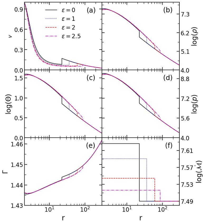
2      S. Patra et al.
obtained metric is characterized by the mass, spin and only one devi-      points and consequently suffer the shock transitions. This eventually
ation parameter. When the deviation parameter is zero, it is reduced       provides new signatures of accretion dynamics in the non-Kerr BH
to the original Kerr metric. Their analysis also inflicts one valuable     spacetime. We show that for a given spin parameter (ak ), the usual
outcome in the calculation of the ISCO and circular photon orbits,         BH accretion solutions continue to present up to a maximum value
and their dependency on the spin and deviation parameters under            of the deformation parameter (εmax ). When ε > εmax , the nature of
this proposed background. They show that, depending on the spin            the solution changes due to the presence of an extra sonic point very
parameter, the central singularity of the spacetime becomes naked for      close to the compact object. This possibly happens as the central
outside observers when the deviation parameter crosses some limit-         source seems to appear as naked singularity (Dihingia et al. 2020)
ing value. Usually, these irregularities in spacetime are described by     which is examined using numerical as well as analytical means. We
the negative precession of the closed timelike orbits, which are the       further calculate a parameter space spanned by the spin (ak ) and
observational signature of the naked singular exotic objects.              the deformation parameter (ε) according to the solution topologies
   Meanwhile, various investigations have been performed on the JP         around either BH or naked singularity state of the central objects.
metric. For example, Bambi (2011) found the restriction to the spin        A comparison of εmax obtained in the pseudo-Newtonian model and
parameter for non-Kerr BHs through the observational inconsistency         analytical approach is presented where good agreement is seen. This
in the radiative efficiency for luminous AGNs. In Bambi et al. (2012),     evidently indicates that the accretion dynamics provides an alterna-
the spacial topology of the event horizon for non-Kerr spacetime has       tive window to distinguish the subtle nature of the compact objects.
been investigated. The properties of the ergosphere and the energy            Finally, we wish to emphasis that the global transonic accretion
extraction by the Penrose process in a rotating deformed BH are            solutions in the deformed Kerr spacetime continue to exist as in the
carried out in Liu et al. (2012). Chen & Jing (2012) analyzed the          case of original Kerr spacetime. From our analysis, two new findings
strong gravitational lensing effect in a background of non-Kerr com-       are imparted. One of them is the multiple critical point solutions
pact objects. Krawczynski (2012) distinguished between the original        including shock transitions. Another one is the existence of naked
Kerr BHs hypothesis and non-Kerr BHs, and tested the no-hair theo-         singularity for non-Kerr spacetime even if the spin parameter ak < 1.
rem through the spectropolarimetric observational data of the black        In the alternative gravity theory of GR, these specific findings can
hole XRBs. A detailed investigation of shadows and restriction to the      be considered observational evidence to distinguish the deformed
spacetime parameters have been presented through the observation           spacetime from the original Kerr spacetime.
of polarization angels in Atamurotov et al. (2013). The inclusion of          This paper is arranged as follows. In Section 2, we develop the
new parametric deviation approach and its challenge to the JP met-         mathematical framework of the accretion disc theory and set up the
ric are encountered in Rezzolla & Zhidenko (2014). A review on             critical point conditions. In Section 3, we present the effect of ε
the signatures of alternative gravity by employing the gravitational       on the sonic point analysis, global flow solutions and modification
waves from the BHs merging is presented in Yagi & Stein (2016).            of the parameter space for the non-Kerr BH. Section 4 analyzes
The simultaneous existence of closed timelike orbits with negative         the shock-induced global accretion solutions and their parameter
precession and shadows is reported for the non-Kerr naked singular         spaces. The dependence of shock properties on ε is also established
spacetime in Bambhaniya et al. (2021). Very recently, the properties       in this section. In Section 5, we show the flow solutions associated
of the accretion disc around a non-Kerr black hole without reflec-         with zero angular momentum flows. In Section 6, we depict how ε
tion symmetry have been revealed in Chen & Yang (2021). All these          incorporates the naked singularity in the system through sonic point
works evidently indicate that the JP metic attracts huge focus on it       analysis and their corresponding transonic solutions. In addition, the
and also gets tremendous success for different applications in grav-       change of parameter space of multiple critical points for non-Kerr
ity. However, to the best of our knowledge, no one has conveyed            naked singularity has been presented in this section. In Section 7, we
the hydrodynamics of the accreting matter in the background of JP          represent the properties of the spacetime parameters in the JP metric.
compact objects. Such deficiency in the literature pushes us to serve      Finally, in Section 8, we present conclusions.
the present work, where we explore, for the very first time, the ac-
cretion dynamics of fluids in a spacetime of alternative gravity. We
expect this analysis will lead to a better understanding of the non-Kerr
spacetime in the light of accretion dynamics.
   In this work, we solve the general relativistic Euler’s equation in
the JP spacetime by utilizing the standard definitions of three veloci-
                                                                           2 ASSUMPTIONS AND GOVERNING EQUATIONS
ties (Lu 1985) in a co-rotating frame. Even in the strong-field regime,
flow equations mimics the Newtonian-like equations and provide the         We present the basic equations governing the accretion flow using
effective potential corresponding to the gravitating object (Dihingia      general relativistic hydrodynamics. To avoid mathematical complex-
et al. 2018b). We derive the radial velocity gradient and temperature      ity, the accretion disc is assumed to remain confine around the equa-
gradient equations using the relativistic equation of state (REoS) that    torial plane of the central object. We further consider the flow to
endure variable adiabatic index (Γ). After developing the mathemat-        be steady, inviscid and advective, where energy dissipations due to
ical framework, our primary motivation is to express the influence         viscosity, thermal conduction, magnetic fields and radiative cooling
of the deformed term on the flow properties. We start our analysis         are neglected.
accommodating the effect of the deformation parameter (ε) on the
nature of critical points and the global transonic solutions around BH.
Next, we separate the parameter space (in angular momentum (λ) -
energy (E) plane) by means of the nature of the solution topologies
and show their modifications with the input parameters. The global
                                                                           2.1 Governing equations
shock solutions, including their inherent properties, have been stud-
ied in detail. An important result is presented where we depict that       In the standard Boyer-Lindquist coordinates (t, r, θ, φ), the deformed
even zero angular momentum flow can possesses multiple critical            Kerr metric (known as JP metric) is expressed as (Johannsen & Psaltis

MNRAS 000, 1–17 (0000)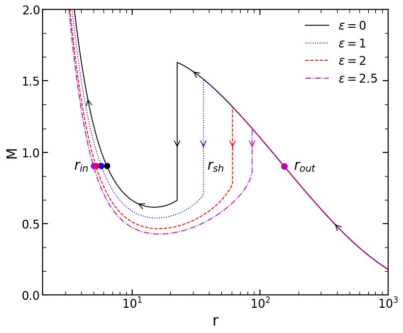
Accretion Dynamics            3
2011),                                                                                                                                           (6)
               2M r                                                           The above relation is explicitly written for our metric (1). Since the
ds2 = −(1 −           ) [1 + h(r, θ)] dt2
                 Σ                                                            motion is considered around the disk equatorial plane, and there are
        4M rak sin2 θ                                                         time translation as well as azimuthal symmetries, the equations (2)
      −                  [1 + h(r, θ)] dtdφ
             Σ                                                                and (3) for i = r are simplified as (Dihingia et al. 2018b, 2020),
          Σ [1 + h(r, θ)]                                               (1)
      +                        dr2 + Σdθ2                                     e + p dρ   de
                                                                                       −    =0                                                   (7)
        ∆ + a2k h(r, θ) sin2 θ                                                  ρ dr     dr

                                      2M r                                    and
      + Σ + a2k [1 + h(r, θ)] (1 +          ) sin2 θ sin2 θdφ2 ,
                                        Σ                                             dv    1 dp     dΦeff
                                                                              γv2 v      +         +       = 0.                                  (8)
where Σ = r    2
                   +a2k   2
                      cos θ and ∆ = r      2
                                               −2M r+a2k . Here, h(r, θ) (=           dr   h1 ρ dr    dr
εM 3 r/Σ2 ) denotes the deformation that accounts the deviation of            For the same reason, i = θ component of equation (3) is trivially
the metric under consideration from the original Kerr metric. And,            satisfied and therefore does not lead to any new equation. However,
ak and M are the spin parameter and the mass of the central object,           for i = φ, equation (3) provides the conservation of specific angular
respectively while ε refers the deformation parameter. In the ε → 0           momentum (Dihingia et al. 2018b), which we already encountered
limit, equation (1) leads to the original Kerr metric. In this work,          through the Killing symmetries in the metric. Following (Chakrabarti
we use G = M = c = 1 unit system, where G and c are the                       1989; Dihingia et al. 2018b, and references therein), we identify Φeff
gravitational constant and the speed of light, respectively.                  in equation (8) as the effective pseudo-potential and is given by ,
   In the relativistic ideal fluid hydrodynamics, the mass conserva-
                                                                              Φeff = 1 + 0.5ln(Φ) .                                              (9)
tion equation [∇k (ρuk ) = 0] and energy-momentum conservation
equation [∇i T ik = 0] take the generalized form of the continuity            For the metric given in equation (1), Φ is given by
and Euler’s equations (Kumar & Chattopadhyay 2017; Dihingia et al.
2018b, 2019a, 2020), and are given by,                                                                       (∆ + a2k h)(1 + h)r
                                                                              Φ=                                                                    .
    h            i                                                                     a2k (r   + 2)(1 + h) − 4ak λ(1 + h) + r3 − λ2 (r − 2)(1 + h)
∇k (e + p)uk = uk ∇k p                                           (2)                                                                            (10)
and                                                                             Integrating the mass conservation equation, we obtain the mass
                                                                              accretion rate (Ṁ ) which is given by (Kumar & Chattopadhyay 2017;
(e + p)uk ∇k ui + ∇i p + ui uk ∇k p = 0.                                (3)   Dihingia et al. 2018b),
                     k
Here e, p and u are the total internal energy, pressure, and four-
                                                                                                   q
                                                                              Ṁ = −4πρvγv H (∆ + a2k h)(1 + h),                             (11)
velocity of the fluid, respectively, and the spacetime indices (i, k)
bear values from 0 to 3. The stationary and axisymmetric spacetime,           where H is the local half thickness of the disc. Following the work
due to its symmetries, is associated with two Killing vectors: η µ = δtµ      of Chattopadhyay & Ryu (2009), we adopt the relativistic equation
and ζ µ = δφµ . The corresponding conserved quantities are given by,          of state (REoS) and pressure (p) as,
−h1 ut = E          and       h1 uφ = L,                                (4)                           ρf               2ρΘ
                                                                                                      e=    and p =        ,                  (12)
                                                                                                       τ                 τ
where h1 = (e + p)/ρ is the specific enthalpy and ρ is the mass
                                                                              where τ = 2 − ξ(1 − 1/χ), the composition ratio ξ = np /ne
density of the fluid. Here, E is the Bernoulli function and L is the
                                                                              and the mass ratio χ = me /mp . The number density and the mass
bulk angular momentum per unit mass of the fluid. The specific
                                                                              of the ith species (electron, proton) are denoted by ni ∈ {ne , np }
angular momentum is defined as λ = L/E = −uφ /ut that remains
                                                                              and mi ∈ {me , mp }, respectively. Moreover, we consider ξ = 1,
conserved along the streamlines of the flow.
                                                                              throughout our analysis. Here the quantity f is obtained in terms of
   Following Lu (1985), we adopt the components of three-velocity
                                                                              dimensionless temperature (Θ = kB T /me c2 , kB is the Boltzmann
in a corotating frame. The azimuthal, polar and radial-component
                                                                              constant and T is the flow temperature in Kelvin) as
of three-velocity are defined as vφ2 = uφ uφ /(−ut ut ), vθ2 =
γφ2 (uθ uθ )/(−ut ut ) and v 2 = γφ2 γθ2 vr2 respectively, where vr2 =

                                                                                                      9Θ + 3             1       9Θ + 3/χ
                                                                              f = (2 − ξ) 1 + Θ                   +ξ       +Θ                   .
ur ur /(−ut ut ). The respective bulk Lorentz-factors (γφ , γθ and                                    3Θ + 2             χ       3Θ + 2/χ
γv ) are expressed as γφ2 = 1/(1 − vφ2 ), γθ2 = 1/(1 − vθ2 ) and                                                                              (13)
γv2 = 1/(1 − v 2 ). As the accretion disk is considered as geomet-
rically thin, we regard the fluid motions around the disc equatorial          For REoS, polytropic index (N ), adiabatic index (Γ) and sound speed
plane (θ = π/2) with vθ = 0 and γθ = 1. Under these assumptions,              (Cs ) are defined as
the angular velocity of the fluid is obtained as (Chakrabarti 1996),                   1 df          1             Γp    2ΓΘ
                                                                              N=            ; Γ = 1 + ; and Cs2 =     =        .                (14)
         φ                                                                             2 dΘ          N            e+p   f + 2Θ
  u          [λ(r − 2) + 2ak ] (1 + h)
Ω= t = 2                                    ,                           (5)      Considering the hydrodynamic equilibrium in the vertical direc-
  u   ak (1 + h)(r + 2) − 2ak λ(1 + h) + r3
                                                                              tion, the local half thickness of the disc (H) is calculated as (Lasota
where h = h(r, θ = π/2) = ε/r3 . The normalization ui ui = −1                 1994; Riffert & Herold 1995; Peitz & Appl 1997),
yields the covariant time-component of four-velocity and is given by                 s         r
(Dihingia et al. 2019a, 2020),                                                          pr3        2r3 Θ
                                                                              H=             =           ,                                       (15)
                                                                                        ρF          τF
ut = γv
   s                                                                          where
                          (∆ + a2k h)(1 + h)r                                             (r2 + a2k )2 + 2∆a2k
×       2
       ak (r + 2)(1 + h) − 4ak λ(1 + h) + r3 − λ2 (r − 2)(1 + h)
                                                                 .            F = γφ2                          .                                (16)
                                                                                          (r2 + a2k )2 − 2∆a2k

                                                                                                                              MNRAS 000, 1–17 (0000)
4 S. Patra et al.
Integrating equation (7) and using equation (12), the mass density 2.2 Critical point conditions
is obtained as (Kumar et al. 2013; Chattopadhyay & Kumar 2013;
In an accretion process around a gravitating object, infalling matter
Dihingia et al. 2020),
starts accreting with negligible radial velocity from the outer edge of
ρ = K exp (k3 )Θ3/2 (3Θ + 2)k1 (3Θ + 2/χ)k2 , (17) the disk (usually far away from the horizon) and remain sub-sonic.
On the other hand, accretion flow enters into the black hole super-
where k1 = 3(2 − ξ)/4, k2 = 3ξ/4, k3 = (f − τ )/(2Θ), and sonically in order to satisfy the inner boundary conditions imposed
K refers the entropy constant. Using equations (11) and (17), we by the event horizon. Since the motion of the flow generally remains
compute the entropy accretion rate as (Chattopadhyay & Kumar smooth everywhere, accreting matter experiences sonic state transi-
2016; Kumar & Chattopadhyay 2017), tion at some point to become transonic Liang & Thompson (1980b);
Abramowicz & Zurek (1981) and such a point is referred as critical
Ṁ
q
Ṁ = = vγv H (∆ + a2k h)(1 + h) point (rc ). At rc , the radial velocity gradient takes (dv/dr)rc = 0/0
4πK (18) (equation 23) form as it must be real and finite, and hence, we obtain
× exp (k3 )Θ3/2 (3Θ + 2)k1 (3Θ + 2/χ)k2 . the critical point conditions by setting D = N = 0 simultaneously
which are given by,
Considering logarithmic derivative of equation (11) and setting the
condition of constant mass accretion rate (i.e., dṀ /dr = 0), the 2
2Csc
temperature gradient is expressed as, vc2 = (26)
(Γc + 1)
dΘ 2Θ
=− and
dr 2N + 1
2 (19)
a2k
γ dv 3ε 1
× v + N11 + N12 − 4 + , Γc + 1
dΦeff
v dr 2r ∆ + a2k h 1+h 2
Csc = ×
2 dr c
where −1
a2k
3ε 1
5 r− a2k (1
+ h) 1 dF (N11 )c + (N12 )c − + ,
N11 = + and N12 = − . (20) 2rc4 ∆c + a2k hc 1 + hc
2r r(∆ + a2k h) 2F dr (27)
1 dF
The explicit form of the quantity F dr
is obtained by taking the where the subscript “c” refers quantities measured at the critical
logarithmic derivative of equation (16) and is given by, point. We evaluate (dv/dr)rc by applying l0 Hôpital’s rule which is
" 0
# obtained as
1 dF 2 0
2 2 2 (r2 + a2k )∆ − 4∆r √
= γφ λΩ + 4ak (r + ak ) , (21) dv −B ± B 2 − 4AC
F dr (r2 + a2k )4 − 4∆2 a4k = , (28)
dr c 2A
where where the resulted form of quantities A, B and C are presented
in Appendix A. In general, critical points are classified in three
0 d∆ different categories. For saddle type critical points, both values of
∆ = = 2(r − 1);
dr (dv/dr)rc are real with opposite sign. For nodal type critical points,
0 dΩ both values of (dv/dr)rc are real and same sign, whereas for O-type
Ω = = −2(1 + h)
" dr # critical point, (dv/dr)rc becomes imaginary. It is noteworthy that
a3k (1 + h) − 2a2k λ(1 + h) + ak [λ2 (1 + h) + 3r2 ] + r2 λ(r − 3) any physically acceptable accretion solution only passes through the
×
[a2k (r + 2)(1 + h) − 2ak λ(1 + h) + r3 ]2 saddle type critical point (Das 2007; Chakrabarti & Das 2004, and
references therein), and hence, in this work, we focus only those
3ε [λ(r − 2) + 2ak ]
− . accretion solutions that possess saddle type critical point (hereafter
r [a2k (r + 2)(1 + h) − 2ak λ(1 + h) + r3 ]2 critical point). We further mention that accretion flow may contain
(22) multiple critical points depending of the flow parameters and flow of
this kind are potentially favourable to contain shock wave (see §4).
Finally, we capitalize equation (14) and obtain the radial velocity
gradient from equation (8) as,
dv N 3 HYDRODYNAMICS WITH DEFORMATION
= , (23)
dr D
In this section, we explore the role of the deformation parameter (ε)
where the explicit form of the denominator D and that of the numer- in deciding the nature of the critical points as well as the accretion
ator N are represented by, solutions in the non-Kerr (deformed) spacetime. While doing this,
we identify the range of parameters that allows accretion solutions
2Cs2
2
D = γv v − (24) around black holes. We also put efforts in examining the nature of
(Γ + 1)v the accretion solutions beyond black hole environment as well.
and
2Cs2 3.1 Critical points analysis
N=
Γ+1 As the accretion solutions embrace the critical points, we start our
(25)
a2k dΦeff
3ε 1 analysis by understanding the nature of critical points. For that we
× N11 + N12 − 4 + − .
2r 2
∆ + ak h 1+h dr calculate the specific energy (Ec ) at a critical point (rc ) by solving
MNRAS 000, 1–17 (0000)Accretion Dynamics 5
Figure 1. Plot of specific energy (Ec ) as the function of critical point locations (rc ) for (a) different angular momentums λ = 2.5, 2.7, 2.9 and 3.1 with
deformation parameter ε = 3, and (b) different deformation parameters ε = 0, 3, 6 and 9 with the specific angular momentum λ = 2.8. Solid, dotted and dashed
curves denote saddle, nodal and O-type critical points, respectively. The dot-dashed horizontal line indicates the specific energy Ec = 1. Here, we choose Kerr
parameter ak = 0. See text for details.
equations (4), (26) and (27) using the global parameters, namely λ, (Θc ) at rc by simultaneously solving equations (4), (14), (26) and
ε and ak , respectively. In Fig. 1, the variation of Ec as a function (27) for a given set of input parameters (λ, E, ak and ε). We employ
of rc is presented for different λ with ε = 3 (see panel (a)) and for Θc and vc as the initial values at rc to simultaneously solve equations
different ε with λ = 2.8 (see panel (b)). Presently, we choose the Kerr (19) and (26) once inward upto the horizon (rH ) and then outward
parameter ak = 0. However, we mention that there are no qualitative upto the outer edge of the disk (redge ). Finally, we join this two parts
differences between the characteristics of critical points for the non- of the solution to obtain the complete radial profiles of velocity (v)
spinning and spinning black holes. Hence, in this work, most of the and temperature (Θ). In Fig. 2, we depict the accretion solutions
analyses have been carried out considering ak = 0, although there (M vs. r) for different ε, where E = 1.001, λ = 2.8 and ak = 0
are instances where results for ak 6= 0 are presented according to the are chosen. In panels (a-d), the variation of Mach number (M ) as
necessity. In the figure, different λ and ε values are marked in the function of radial distances (r) is presented for ε = 0, 3, 6 and 9,
respective panels. We use black, blue, red and orange curves for λ respectively. Here, the solid curve represents the accretion solution
= 2.5, 2.7, 2.9 and 3.1 respectively. The same color curves are used whereas dashed curve denotes the corresponding wind solution. In
to represent results for ε = 0, 3, 6, and 9, respectively. In each panel, the figure, filled circles refer the critical points, where inner (rin ) and
a given curve is generally comprised with saddle, nodal and O-type outer (rout ) critical points are marked. We observe that for ε = 0,
critical points and they are demonstrated by the solid, dotted and the flow passes through the outer critical point at rout = 198.6333
dashed curves respectively. Moreover, these critical points appear in and connects the outer edge of the accretion disc (redge = 1000)
sequence as saddle-nodal-spiral-nodal-saddle as rc is increased. In to the black hole horizon (rH ) (see panel (a)). As the deformation
addition, we observe that all curves have an asymptotic behaviour parameter is increased (say ε = 3) keeping other input parameter
towards Ec ' 1 (dash-dotted horizontal line) for larger values of unchanged, inner critical point is appeared at rin = 5.7136 along
rc irrespective of λ and ε values. Depending on Ec , λ and ε, flow with the outer critical point at rout = 198.5498. Interestingly, the
may contain either single or multiple critical points. Usually, critical solution passing through the outer critical point continues to connect
points formed near and far away from the the horizon are called as rH and redge , however the inner critical point solutions fail to do so
inner (rin ) and outer critical points (rout ), respectively. It is evident at it terminates at a radius (rt = 20.3336) in between inner and
from the figure that there exists a range of Ec that yields multiple outer critical points as rin < rt < rout as shown in panel (b). For
critical points and such energy range is strictly depends on λ and ε ε = 6, the nature of the flow solution remains qualitatively similar
values. Following this, in §3.3, we put effort to identify the effective to panel (b) although rt = 77.7947 is increased (see panel (c)).
region of the parameter space based on the nature of the accretion We wish to emphasize that solutions presented in panel (b-c) may
solutions. Overall, it is now evident that ε, λ and Ec play pivotal experience shock transition and we plan to discuss it elaborately in
role in determining the nature of the critical points and its associated §4. With the further increase of deformation parameter ε = 9, the
properties. solution characteristics are changed completely as shown in panel
(d). We find that the solution passing through rin = 3.4628 smoothly
connects redge to rH , but the possesses rout = 198.3757 fails to do
so. Hence, it is evident that ε plays a decisive role in determining
3.2 Effect of ε on global accretion solutions
the nature of the accretion solutions around the central object under
Here, we examine the impact of ε on the accretion solutions. While consideration.
doing so, we calculate the location of the critical point (rc ), and the
corresponding radial velocity (vc ) and dimensionless temperature
MNRAS 000, 1–17 (0000)6 S. Patra et al.
Figure 2. Plot of Mach number M (= v/Cs ) as a function of radial distance r. Solid and dashed curves denote the accretion solution and wind solution,
respectively. Filled circle denotes the critical point. Here, we choose E = 1.001, λ = 2.8 and ak = 0. Result in panels (a), (b), (c) and (d) are for ε = 0, 3, 6
and 9, respectively. See the text for details.
3.3 Parameter space based on nature of accretion solutions and rout = 355.8871). For (λ, E) = (2, 1.007), we display the ac-
cretion solutions in inset panel (c). The sonic points are obtianed as
In this section, we separate the effective region of the parameter space rin = 1.2606, rs = 5.6399 and rout = 34.3714. However, the solu-
(in λ − E plane) according to the nature of the accretion solutions. tions in panel (d) promote inner critical point only (rin = 1.2575). It
The obtained results are plotted in Fig. 3(A), where four regions, is to be noted that even for the highly rotating black holes, the flow
namely (a), (b), (c) and (d) are identified according to the nature of solutions are similar to that of the nonrotating black holes.
the solution topologies. We present their respective solutions in inset
panels. Here, the Mach number (M = v/Cs ) is plotted with the We additionally figure out various flow parameters (defined in
radial distances (r) in each panel. The accretion and wind solutions equations (12), (14), (18) and (23)) in Fig. 4, associated with the
are denoted by black (solid) and blue (dashed) lines respectively, and global accretion solution in inset panel (a) of Fig. 3(A). Moreover,
the filled circles are used for the saddle type critical points. Note that we consider that the flow enters at the outer edge redge = 1000 of the
all the solutions which have been drawn in the inset panels contain accretion disc. The evolution of the bulk velocity (v), dimensionless
the saddle type critical points only. The area with in red (dashed) temperature (Θ), mass density (ρ), local pressure (p), adiabatic index
line represents the region (b) and the remaining area with in the (Γ) and entropy accretion rate (Ṁ) as function of radial coordinates
grey (solid) line represents the region (c). The notion behind the (r) are presented in panels (a), (b), (c), (d), (e) and (f) respectively.
finding of the region (b) is that the entropy accretion rate at the inner It is depicted that all inspected quantity increases monotonically
critical point is more compared to the outer critical point; however, (see panels (a) - (d)) as we move towards the inner egde until it
for region (c), the adopted logic is just the reverse one. For panel gently fall into the black hole horizon. However, the adiabatic index
(a), we choose the flow parameters as λ = 2.5 and E = 1.001. In decreases (see panel e) with the decrease of radial coordinates due
this case, the critical point is found at rout = 203.562, which is a the rise of temperature. We calculate the entropy accretion rate as
saddle one. The solutions corresponding to panel (b) are obtained for Ṁ = 2.7202 × 10⁷ from the panel (f), revealing a constant quantity
input parameters (λ, E) = (2.80, 1.001), where the critical points are for a particular solution.
obtained at rin = 4.5132 (saddle-type), rs = 13.0295 (O-type) and Variability in the parameter space of a set of parameters corre-
rout = 198.4749 (saddle-type). In panel (c), we plot the solutions sponding to given other parameters is quite often in the context of
while choosing the flow parameters as (λ, E) = (3, 1.001). Here, accretion dynamics. To acknowledge this identity, we represent the
we calculate the critical points as rin = 4.0795 (saddle-type), rs = alteration of parameter space associated with multiple critical points
17.0861 (O-type) and rout = 194.5943 (saddle-type). Finally, we (saddle types) in the λ−E plane for different ε in Fig. 5. We consider
find the solution in panel (d) for injected flow parameters (λ, E) = the Kerr parameter ak = 0 and mark the various ε in this panel. Dif-
(3, 1.0045) and evaluate the critical point as rin = 4.0445 (saddle- ferent potential regions are obtained while using blue (solid), black
type). Therefore, if we consider any flow parameter (λ, E) from the (dashed), magenta (dotted) and red (dash-dotted) lines for ε = 0, 5, 10
regions (a) and (d), the solution possesses one critical point only. and 15.2 respectively. Here, we observe that the parameter space is
However, any flow parameters (λ, E) from the regions (b) and (c) shifted towards lower angular momentum and higher energy with the
provide the solutions containing both the critical points. increase of the deformation parameters for a specific value of Kerr
Now we investigate the black hole solutions for spin parameter parameter. However, it is understandable that more deformations to
ak = 0.99, checking whether it is consistent or not. In Fig. 3(B), spacetime endorse the larger areas in the parameter space. Interest-
we separate the parameter space as (a), (b), (c) and (d) by follow- ingly, a small nozzle-shaped area for multiple critical points is found
ing different solution topologies for a rapidly rotating black hole at zero angular momentum for ε = 15.2. It is essential to highlight
(ak = 0.99) and capitalize ε = 0.015. Here, all lines and dots bring that choice ε = 15.2 is not arbitrary; it provides the minimum value
identical information as in panel (A). The global accretion solution of the deformation parameter, which delivers a small energy range
associated with the inflow parameters (λ, E) = (1.8, 1.015) has been corresponding to the multiple sonic points for λ = 0. When we take
presented in inset panel (a), which contain only outer critical point any ε beyond the value mentioned above, we can carry out the mul-
rout = 357.8267. In panel (b), we depict the solutions correspond- tiple sonic points even for λ = 0; obviously, it depends on the spin
ing to the input parameters (λ, E) = (1.97, 1.0005). In this case, parameter. This finding is entirely new, and no one ever has reported
solutions possess multiple critical points (rin = 1.3283, rs = 4.433 it in the literature. But the big question is whether the associated
MNRAS 000, 1–17 (0000)Accretion Dynamics 7
Figure 3. Division of parameter space in λ − E plane according to the nature of the flow solution topologies. For panel (A) and (B), we choose (ak , ε) = (0, 5)
and (0.99, 0.015), respectively. In each plot, four regions are marked as (a), (b), (c), (d) and the corresponding solutions are shown in the inset panels. See text
for details.
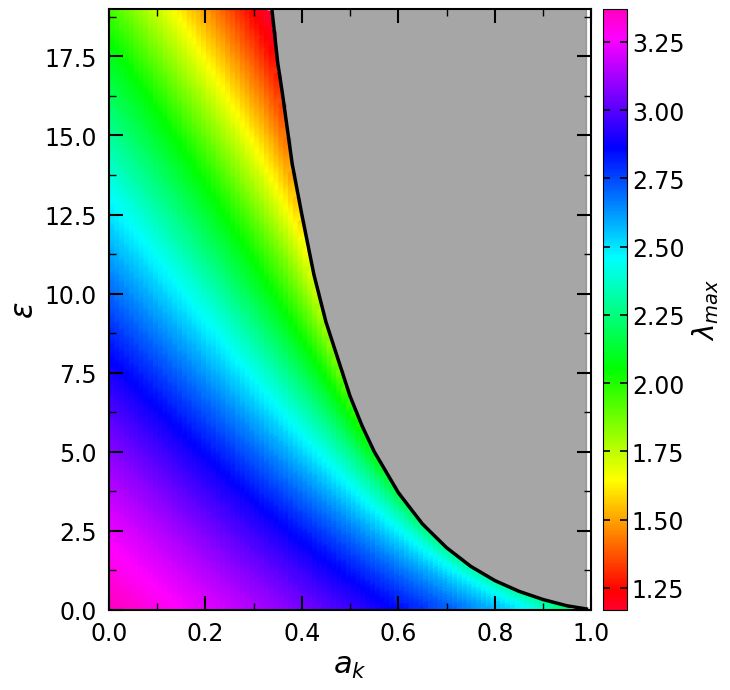
Figure 5. Modification of the parameter space in λ − E plane for multiple
critical points with deformation parameter (ε). Here, we fix Kerr parameter
Figure 4. Variation of (a) bulk velocity (v), (b) temperature (Θ), (c) density ak = 0. Regions bounded with blue (solid), black (dashed), magenta (dotted)
(ρ), (d) pressure (p), (e) adiabatic index (Γ), (f) entropy accretion rate (Ṁ) and red (dash-dotted) curves are for ε = 0, 5, 10 and 15.2, respectively. See
with the radial distances (r). Here, we choose λ = 2.5, E = 1.001, ak = 0 text for details.
and ε = 5, respectively. See text for details.
accretion solutions for zero angular momentum are consistent with in the λ − E plane for different Kerr parameters (ak ) with ε = 0.02.
the general black hole solutions corresponding to non-zero angu- In this panel, we mark ak values as well. The functional domains
lar momentum. Section 5 has discussed a detailed analysis on this are separated using the black (solid), blue (dashed) and red (dotted)
subject. curves correspondings to ak = 0, 0.5 and 0.99 respectively. It is
In the above case, we discovered the parameter space for the non- clarified that the segment within a curve moves into the lower angular
rotating black hole. Now it’s time to invent the effect of the non-zero momentum and higher energy sites. Moreover, the area under an
spin on parameter space for a given deformation parameter. Here, identified province is more in the case of a rapidly rotating object
we fix ε = 0.02, which grants the previously discussed accretion than that of a moderately spinning black hole. Therefore, the above
solutions for the black hole of different spins. In Fig. 6, we study the two analyses suggest that the Kerr parameter and the deformation
parameter space modification for saddle type multiple sonic points parameter play the equivalent role in controlling the parameter space.
MNRAS 000, 1–17 (0000)8 S. Patra et al.
Figure 6. Modification of the multiple critical points parameter space in
λ − E plane with Kerr parameter (ak ). Here, we choose the deformation
parameter as ε = 0.02. Regions bounded with black (solid), blue (dashed) .
and red (dotted) curves are for ak = 0, 0.5 and 0.99, respectively. See text
for details. Figure 8. Variation of (a) radial velocity (v), (b) density (ρ), (c) temperature
(Θ), (d) pressure (p), (e) adiabatic index (Γ) and (f) entropy accretion rate
(Ṁ) as a function of radial coordinate (r) for accretion solution containing
shock. Here, we choose ak = 0, ε = 3, E = 1.0005 and λ = 3, respectively.
In each panel, vertical line represents the radius of the shock transitions at
rsh = 50.1706. See text for details.
happen in the flow variables when the centrifugal repulsion becomes
comparable to the black hole’s gravitational pull. Therefore, at the
centrifugally driven shock location, fluid has to simultaneously sat-
isfy the following relativistic shock conditions (Taub 1948):
[ρur ] = 0; (e + p)ut ur = 0;
(29)
[(e + p)ur ur + pg rr ] = 0,
along with the pre-mentioned necessary condition. Here the terms
in the square brackets refer to the difference in respective quantities
before and after shock. In Fig. 7, we represent the global accretion
solutions which comprise the shock transition for fluid parameters
Figure 7. Example of a shock induced global accretion solution around black (λ, E) = (3, 1.0005). Here, we choose ak = 0 and ε = 3. In this
hole where the variation of Mach number (M ) with the radial coordinates figure, the Mach number (M ) is plotted with the radial distances
(r) is shown. Here, we choose ak = 0, ε = 3, λ = 3 and E = 1.0005, (r). It is observed that the solution (solid, grey) accreting through
respectively. Vertical arrow indicates the location of the shock transition at the outer critical point rout = 339.7504 builds a steady connection
rsh = 50.1706. Arrows denote the overall flow motion towards the black between the outer edge accretion disc and the horizon. However,
hole. See text for details. the solution (dashed, magenta) passing through the inner critical
point rin = 4.7916 is closed one and connects the horizon only.
The global shock solutions is intimated by the red (solid) curve and
4 ACCRETION SOLUTIONS WITH SHOCK TRANSITIONS
the vertical line denotes the shock transition at the shock location
In Subsection 3.2, we mentioned about the possibility of existence rsh = 50.1706, which is calculated by using (29). The arrow heads
of shock solution as the necessary (but not sufficient) condition for indicate the overall flow direction.
shock transition – possession of higher entropy content in the sub- Shock has a significant impact on the fluid and disc parameters.
sonic branch compared to the supersonic branch – was shown to be Here, we invent how the shock transitions affect the flow variables.
satisfied. In principle, the solution enters subsonically from the outer In Fig. 8, we illustrate the dynamics of several flow parameters cor-
edge of the disc which becomes supersonic after being passed through responding to the global shock solution of Fig. 7. We depict the
the external critical point and continues to accreate towards the hori- variation of radial velocity (v), mass density (ρ), dimensionless tem-
zon. In the meantime, discontinuous shock transitions (Fukue 1987; perature (Θ), local pressure (p), adiabatic index (Γ) and entropy
Chakrabarti 1989; Yang & Kafatos 1995; Chakrabarti & Das 2004; accretion rate (Ṁ) with the radial coordinate (r) in panels (a), (b),
Chattopadhyay & Kumar 2016; Kumar & Chattopadhyay 2017; Di- (c), (d), (e) and (f) respectively. In panel (a), it is explicated that
hingia et al. 2018b,c; Dihingia et al. 2018a; Dihingia et al. 2019a,b) the radial velocity experiences a sudden jump at the shock location.
MNRAS 000, 1–17 (0000)Accretion Dynamics 9
Figure 9. Variation of Mach number (M ) with the radial coordinates (r)
for different deformation parameters (ε). Here, we choose ak = 0, λ = 3
and E = 1.0013. Vertical arrows indicate the radius of the shock transition
at rsh = 22.5278, 36.1334, 61.0066 and 86.8639 corresponding to ε =
0, 1, 2 and 2.5, respectively. Critical points (rin and rout ) are annotated by .
the filled circles. See text for details.
Figure 10. Variation of (a) radial velocity (v), (b) density (ρ), (c) temperature
(Θ), (d) pressure (p), (e) adiabatic index (Γ) and (f) entropy accretion rate
Therefore, the fluid gets compressed and correspondingly a sharp (Ṁ) as a function of radial coordinates (r) in a spacetime with different defor-
mation parameters (ε). Each black (solid), blue (dotted), red (dashed) and ma-
transition in the local density is detected in panel (b). It is interpreted
genta (dash-dotted) curves are used for ε = 0, 1, 2 and 2.5, respectively. Here,
from the panel (c) that the temperature changes substantially when we choose (λ, E) = (3, 1.0013), and ak = 0. In each panel, shock locations
the flow transitions to the subsonic arm from the supersonic one due are indicated by the vertical lines at rsh = 22.5278, 36.1334, 61.0066 and
to the conversion of kinetic energy into thermal energy. Hence, the 86.8639, respectively. See text for details.
fluid components (electrons, ions, etc.) collide more and stimulate the
high-pressure content after the shock transition (see panel (d)). As the
temperature in the post-shock disc is higher than the pre-shock disc,
such discontinuity in other temperature-dependent quantities is also shock locations are moving away from the black hole horizon with
exposed (see panels (e) and (f)). However, after shock transition, the the increase of deformation parameter. For this specific case the
electron clouds in the post-shock disc become ultra-relativistic due shock locations are computed as rsh = 22.5278, 36.1334, 61.0066
to high temperature and trigger the inverse Compton effect to soft and 86.8639 corresponding to ε = 0, 1, 2 and 2.5 respectively.
photons coming from the pre-shock disc; hence, produce the hard The vertical lines indicate the discontinuous shock transitions from
and non-thermal flux distribution in the electromagnetic spectrum the supersonic components into the subsonic components at their
of the accretion disc. Not only that, several numerical simulations respective shock locations mentioned above. Moreover, we notice
show that extremely thermalized electrons are deflected along both that the change of the Mach numbers across the shock transitions
directions of the BH’s rotation axis and thereby address the bipolar skid into the lower values with increased spacetime deformations.
relativistic jets (Molteni et al. 1994; Chattopadhyay & Das 2007; However, shock fonts seem to disappear if we deform the spacetime
Das & Chattopadhyay 2008; Kumar & Chattopadhyay 2013; Das more and flow smoothly collects towards the horizon instead of goes
et al. 2014; Kumar et al. 2014; Kumar & Chattopadhyay 2017). This through the shock transition. In this case, shock conditions (29) are
analysis intimates that the shock transitions play a crucial role in not satisfied even though the subsonic unit holds a greater entropy
controlling the flow parameters and the black hole’s spectral prop- content than the supersonic unit.
erties. So far, we have not confessed the the role of ε governing In Fig. 10(a), we represent the bulk radial velocity (v) profile with
the shock-induced global accretion solutions and flow parameters. the radial coordinates (r) corresponding to the above mentioned de-
The following subsection shape the above mentioned requirement formation parameters which embrace the shock fonts. Furthermore,
through explicit analysis. we consider the same set of input parameters as we took in Fig. 9.
As the shock fonts move away from the horizon, the vertical jumps
in v decreases with the increase of ε. After a specific value of ε
(we call this as εc ) shock transitions cease to exist and smooth ac-
4.1 Effect of ε on global shock solutions and shock properties
cretion through the extreme critical point will continue again. The
This subsection starts our discussion by considering the black hole exact value of εc is not calculated yet; however, its accurate estima-
of spin ak = 0. Here, we assume the flows entered at the outer edge tion will be given later when discussing the shock properties. We
redge = 300 with the energy E = 1.0013 and angular momentum also characterise other flow parameters for the shock solutions corre-
λ = 3. In Fig. 9, we represent the variation of Mach number (M ) sponding to the input parameters as in Fig. 10(a). The mass density
as the function of radial distances (r) for different ε. The black (ρ), dimensionless temperature (Θ), local pressure (p), adiabatic in-
(solid), blue (dotted), red (dashed) and magenta (dash-dotted) curves dex (Γ) and entropy accretion rate (Ṁ) are plotted as a function of
are used for ε = 0, 1, 2 and 2.5 respectively. The sonic points r in Fig. 10(b), (c), (d), (e) and (f) respectively. In all panels, we use
are spotted by the filled circles corresponding to different ε. The black (solid), blue (dotted), red (dashed) and magenta (dash-dotted)
MNRAS 000, 1–17 (0000)10 S. Patra et al.
Figure 11. Variation of (a) shock location (rsh ), (b) compression ration (R) Figure 12. Variation of (a) shock location rsh , (b) compression ration (R) and
and (c) shock strength (S) with the deformation parameters (ε). Black (solid), (c) shock strength (S) as a function of the deformation parameters (ε). Black
red (dotted), blue (dashed), orange (dash-dotted) and magenta (long dashed) (solid), red (dotted), blue (dashed), orange (dashed-dotted) and magenta (long
curves denote results for λ = 3, 3.025, 3.05, 3.075 and 3.1, respectively. dashed) curves are represented for E = 1.0011, 1.0013, 1.0015, 1.0017 and
Here, we choose ak = 0 and E = 1.0012. See text for details. 1.0019, respectively. Here, we fix ak = 0 and λ = 3. See text for details.
curves curves for ε = 0, 1, 2 and 2.5 respectively. The difference in density Σ ∼ ρH (Chakrabarti & Das 2001), we obtain the expression
entities across the shock transition become less when the deformation of R at the shock location (rsh ) with the help of (11) as (Das 2007;
in the spacetime is increased due to the movement of shock locations Das & Chakrabarti 2008; Sarkar et al. 2018; Sarkar & Das 2018),
towards the outer edge of the accretion disc. This analysis glimpse
Σ+ (rsh ) ρ+ (rsh )H+ (rsh ) v+ (γv )+
the consequence of the deformation parameter on the dynamics of R= = = , (30)
global shock solutions and flow variables but is unable to provide Σ− (rsh ) ρ− (rsh )H− (rsh ) v− (γv )−
complete information. Next, to shape our objective more powerfully, where − and + refer to the quantities before and after shock. In
we focused on the shock properties. Fig. 11(b), we depict the variation of R as function of ε for the same
A detailed analysis of the shock properties has been done here. We set of input parameters as in Fig. 11(a). Here, the compression ratio
explore various shock properties corresponding to different angular decreases with the increase of deformation parameter. This result is
momentum (λ) flows of energy E = 1.0012, injected at the outer quite expected because when the shock fonts move towards the outer
edge redge = 1000 of the accretion disc. The variation of shock edge, the compression of flow in the post-shock region becomes less
location (rsh ) with ε is presented in Fig. 11(a). We apply the black (see Fig. 10b). To understand the temperature jump at the shock
(solid), red (dotted), blue (dashed), orange (dash-dotted) and magenta transition, we define the shock strength (S) as the ratio of the pre-
(long dashed) curves for λ = 3, 3.025, 3.05, 3.075 and 3.1 respectively. shock Mach number (M− ) to the post-shock Mach number (M+ ).
It is found that the shock location is increased with the increase of ε for In Fig. 11(c), we analyze the variation of the shock strength (S)
a given λ. When the deformation parameter exceeds a critical value with ε. Here, we consider the same input parameters, line styles and
(εc ), shock solution does not exist due to the violation of conditional line colors as used in Fig. 11(a) and (b). The result explicits that
relations at the shock location. A sophisticated calculation leads the the shock strength decreases with the increase of ε. As the shock
values of εc are 2.82, 2.47, 1.8, 1.43, and 0.81 for the respective λ locations step away from the horizon, we would expect the shock
mentioned here. The decrease in εc is noticed for the high angular strength to decrease and hence our analysis is precisely justified here
momentum flows when (ak , E) are fixed. Hence, εc is not a universal (see Fig. 10c). The next paragraph will stick to shock properties
quantity and it strongly depends on the injected input parameters. We analysis, setting λ as a universal parameter instead of E.
also notice that the shock locations advance towards the outer edge In Fig. 12, we explore the variation of the shock variables with
with the increase of λ for a given ε. This outcome implies that the ε for flows injected with identical angular momentums λ = 3 but
shock solutions are probably driven by centrifugal repulsion. As we possessing different energies (E). Here, we consider the flows en-
mentioned earlier, the flow density and temperature are substantially ter at redge = 1000 and choose ak = 0. Various shock properties
increased in the post-shock region due to fall off the radial velocity (rsh , R and S) are plotted in panels (a), (b) and (c) respectively. In
at the shock location. Therefore, it is significant to investigate the each panel, we employ the black (solid), red (dotted), blue (dashed),
density and temperature distributions accross the standing shock. We orange (dash-dotted) and magenta (long dashed) curves correspond-
define the compression ratio (R) as the ratio of post-shock surface ing to E = 1.0011, 1.0013, 1.0015, 1.0017 and 1.0019 respectively.
density (Σ+ ) to pre-shock surface density (Σ− ). Since the surface For a fixed E, the shock fonts are shifted outward from the central
MNRAS 000, 1–17 (0000)Accretion Dynamics 11
Figure 14. Modification of shock parameter space in λ − E for different Kerr
Figure 13. Modification of the shock parameter space in λ − E plane as a
parameters (ak ) for ε = 0.02. Black (solid), blue (dashed) and red (dotted)
function of deformation parameter (ε) for ak = 0. Regions bounded with
lines are used for ak = 0, 0.5 and 0.99, respectively. See text for details.
blue (solid), black (dashed), magenta (dotted) and red (dash-dotted) curves
are obtained for ε = 0, 5, 10 and 15, respectively. See text for details.
(solid), blue (dashed) and red (dotted) lines have been sponsored to
object with the increase of ε. However, the standing shock transitions characterize the valid regions for shock transitions corresponding to
monotonically wipes out as one increase ε. When ε > εc , shock ak = 0, 0.5 and 0.99 respectively, and Kerr parameters are appropri-
conditions are failed to maintain, hence shock solutions disappear. ately annotated. We observe that the parameter space moves into the
Here, we also explicitly calculate the quantity εc as 3.04, 2.68, 2.03, lower angular momentums and higher energies zone as we increase
1.61, and 1.07, respectively associated with the energies as men- black hole spin for a given deformation parameter. As the shock
tioned earlier. It is to be noticed that εc decreases with the increase parameter space is the shrink version of the whole multiple critical
of energies and analogously verifies the preferential dependence of point parameter space, its alteration process is not surprising because
εc on the initial parameters. Moreover, the shock location increases the entire parameter space for multiple sonic points, as discussed in
with the increase of energy for a fixed deformation parameter. We Subsection 3.3, is shifted accordingly.
also observe that the compression ratio and shock strength decreases
with the increase of ε due to less flow compression towards outer
edge. Following the above studies, we should mention that without
knowing the parameter space that encompasses the shock solutions, 5 FLOW SOLUTIONS CORRESPONDING TO λ = 0
playing with any analysis connected to shock transitions is relatively There are few unique interesting features are being observed here in
obscure, especially when dealing with the larger span of the param- accretion flow due to the deformation in the spacetime which were
eter space. Once we finish it, our job becomes more accessible, and absent in Kerr spacetime. Presence of such properties clearly isolates
also, we can call any parameters during the investigation. We will the central object from the usual Kerr. In this section we will discuss
calculate the shock parameter space in the next subsection. one of them.
We have already encountered the multiple sonic points for flow
with zero angular momentum in Subsection 3.3. In this analysis, we
4.2 Shock parameter space
examine the presence of accretion solutions associated with these
We now estimate the shock parameter space to enlarge the shock sonic points and remark on them. We assume that the flows enter at
identity. Here, we first characterise the effective regions of the pa- the extreme edge redge = 1000 with the angular momentum λ = 0.
rameter space corresponding to different ε while keeping ak fixed. However, the choice of deformation parameters must be ε ≥ 15.2
In Fig. 13, we find the shock parameter space in λ − E plane for four for ak = 0, as mentioned before. Let us initiate our survey with
different ε = 0, 5, 10 and 15 respectively with ak = 0. Identified the global accretion solutions for (ε, E) = (16, 1.017) in Fig. 15(a),
provinces are bounded with the blue (solid), black (dashed), magenta where the Mach number (M ) is sketched with the radial locations
(dotted) and red (dash-dotted) curves corresponding to respective ε. (r). In this case, solid and dashed curves have been applied to sig-
It is observed that the area under the curve increases with the increase nify the accretion and wind solutions respectively. We use the filled
of deformation parameters. Additionally, the shock parameter space dots corresponding to the saddle type critical points calculated here.
is shifted towards the lower angular momentums and to the higher It is clarified that the solutions occupy only the outer sonic point
energies as deformation in the system increases for a given spin of (rout = 19.8723) and join the exterior part of the accretion disc to
the black hole. the black hole horizon. The entropy accretion rate at the sonic point
Next we study the modification of the shock parameter space for is calculated as Ṁout = 20.5276 × 10⁷ . In Fig. 15(b), we plot the
different ak , but this time ε is taken as constant. Here, we pick up accretion solutions associated with (ε, E) = (17, 1.017) and interpret
ε = 0.02, which holds a similar cause as in Fig. 6. We represent the that the solutions won both inner and outer critical points. The criti-
shock parameter space in λ−E plane for distinct ak in Fig. 14. Black cal points are computed as rin = 4.0993 (saddle-type), rs = 5.3533
MNRAS 000, 1–17 (0000)12 S. Patra et al.
Figure 15. Variation of Mach number (M ) with the radial distances (r) for zero angular momentum (λ = 0) flow. Results are depicted in the panels (a), (b),
(c), (d) and (e) corresponding to (ε, E) = (16, 1.017), (17, 1.017), (18, 1.017), (18.95, 1.019) and (18, 1.03), respectively. Solid and dashed curves denote the
accretion and wind solutions. Critical points are marked by the filled circles. The shock transition is represented by the solid vertical arrow (red) at rsh = 8.7829.
Here, we choose ak = 0. See text for details.
(O-type) and rout = 19.6517 (saddle-type). In this case, the solutions
flowing down the external sonic point are connected with the central
singular point. But the solutions passing through the inner sonic point
seem to form a closed loop near the horizon. The entropy accretion
rates in subsonic and supersonic branches are Ṁin = 24.7699 × 10⁷
and Ṁout = 20.4652 × 10⁷ respectively. Since the entropy con-
tent for the inner one is higher than the outer one, the solution
may experience a shock transition and attains both critical points.
However, we do not compute the global shock solutions in this
regard. For shock-induced global accretion solution, we set (ε, E)
= (18, 1.017). In Fig. 15(c), the red (solid) curve illustrates shock
solution in association with the background general accretion solu-
tions. The satisfied shock conditions at rsh = 8.7829 and the result
Ṁin (22.6956 × 10⁷ ) > Ṁout (20.4013 × 10⁷ ) lead the sharp jump
into the subsonic branch from the supersonic branch, which has been
presented by the vertical line in this panel. Location of two saddle-
type sonic points are given by rin = 3.8059 and rout = 19.4199 and
the spiral one is obtained as rs = 6.0624. An exhibition of accretion
solutions for (ε, E) = (18.95, 1.019) has been done in Fig. 15(d). In
this case, the solutions possess multiple critical points (rin = 3.636,
Figure 16. Variation of specific energy (Ec ) with the critical points (rc ) for
rs = 6.8765 and rout = 17.0132) and deliver the higher entropy
different angular momentums (λ). Here, we choose the Kerr parameter ak =
content for external component (Ṁout = 22.1992 × 10⁷ ) compared 0.99 and the deformation meter ε = 0.03. Saddle, nodal and O-type critical
to the internal one (Ṁin = 21.3056 × 10⁷ ). The solutions passing points are indicated with the solid, dotted and dashed curves. Horizontal line
through the inner critical points behave differently due to their ex- (dash-dotted, magenta) is plotted at the specific energy Ec = 1. See text for
tension through the outer edge towards the horizon. However, the details.
solution going down the outer sonic point is closed and disconnects
the black hole’s horizon with the outer edge. We notice that the outer
sonic points and shock locations are constructed efficiently close to 6 DEFORMATION PROVIDES NAKED SINGULARITY
the horizon for λ = 0 case (Bondi flows). Therefore, all the pre-
In deformed Kerr spacetime, the flow solutions associated with the
requisites of the advection-dominated accretion flows (ADAF) are
central object can behave differently depending on ε for a particular
maintained here. At last, we illustrate another solution correspond-
ak . One of such instance has been explored in the last section. An
ing to (ε, E) = (18, 1.03), which provides only inner (rin = 3.6695)
elaborate discussion on the dependency between ak and ε, which
sonic point (see Fig. 15e). Here, the entropy accretion rate at the
separates those unfamiliar solutions from the usual black hole solu-
inner critical point is evaluated as Ṁin = 27.1305 × 10⁷ and also
tions, will be presented now. Here, we impose the contribution of the
observed that the subsonic solutions at redge are turned into the super-
deformation parameter on the overhead objective.
sonic flows when it crosses rin . This analysis depicts that for λ = 0
flows, we get the different accretion solutions in addition to the global
shock solutions. Most importantly, our new identifications are the ex-
6.1 Impact on the sonic points
istence of the multiple sonic points solutions for “Bondi flows”, and
these solutions can advertise the considerably deformed Kerr black Whenever we have investigated for a rapidly rotating black hole (ak =
holes due to the higher values of ε. When we consider any non-zero 0.99), we have taken ε = 0.02, and the justification behind it has been
spin parameters, we anticipate that the above solutions to appear for mentioned several times. In this section, we consider ε = 0.03 (one
the lower values of ε. Overall, this analysis has a direct influence on of the higher values compared to taken in last discussions). To inflict
identifying the non-Kerr BHs. our analysis, we display the variation of the specific energy (Ec )
with the critical point coordianates (rc ) for different specific angular
momentum (λ) in Fig. 16. We use the black, blue, red and orange
MNRAS 000, 1–17 (0000)You can also read