A simplified atmospheric boundary layer model for an improved representation of air-sea interactions in eddying oceanic models: implementation and ...
←
→
Page content transcription
If your browser does not render page correctly, please read the page content below
Geosci. Model Dev., 14, 543–572, 2021
https://doi.org/10.5194/gmd-14-543-2021
© Author(s) 2021. This work is distributed under
the Creative Commons Attribution 4.0 License.

A simplified atmospheric boundary layer model for an improved
representation of air–sea interactions in eddying oceanic models:
implementation and first evaluation in NEMO (4.0)
Florian Lemarié1 , Guillaume Samson2 , Jean-Luc Redelsperger3 , Hervé Giordani4 , Théo Brivoal2 , and
Gurvan Madec5,1
1 Univ. Grenoble Alpes, Inria, CNRS, Grenoble INP, LJK, 38000 Grenoble, France
2 Mercator Océan, Toulouse, France
3 Univ. Brest, CNRS, IRD, Ifremer, Laboratoire d’Océanographie Physique et Spatiale (LOPS), IUEM, Brest, France
4 Centre National de Recherches Météorologiques (CNRM), Université de Toulouse, Météo-France, CNRS, Toulouse, France
5 Sorbonne Universités (UPMC, Univ Paris 06)-CNRS-IRD-MNHN, LOCEAN Laboratory, Paris, France

Correspondence: Florian Lemarié (florian.lemarie@inria.fr)

Received: 24 June 2020 – Discussion started: 6 August 2020
Revised: 6 November 2020 – Accepted: 4 December 2020 – Published: 27 January 2021

Abstract. A simplified model of the atmospheric boundary         and ABL–sea-ice couplings. With respect to these metrics,
layer (ABL) of intermediate complexity between a bulk pa-        our results show very good agreement with observations and
rameterization and a three-dimensional atmospheric model is      fully coupled ocean–atmosphere models for a computational
developed and integrated to the Nucleus for European Mod-        overhead of about 9 % in terms of elapsed time compared
elling of the Ocean (NEMO) general circulation model. An         to standard uncoupled simulations. This moderate overhead,
objective in the derivation of such a simplified model, called   largely due to I/O operations, leaves room for further im-
ABL1d, is to reach an apt representation in ocean-only nu-       provement to relax the assumption of horizontal homogene-
merical simulations of some of the key processes associated      ity behind ABL1d and thus to further improve the realism
with air–sea interactions at the characteristic scales of the    of the coupling while keeping the flexibility of ocean-only
oceanic mesoscale. In this paper we describe the formula-        modeling.
tion of the ABL1d model and the strategy to constrain this
model with large-scale atmospheric data available from re-
analysis or real-time forecasts. A particular emphasis is on
the appropriate choice and calibration of a turbulent clo-       1   Introduction
sure scheme for the atmospheric boundary layer. This is a
key ingredient to properly represent the air–sea interaction     Owing to advances in computational power, global oceanic
processes of interest. We also provide a detailed descrip-       models used for research or operational purposes are now
tion of the NEMO-ABL1d coupling infrastructure and its           configured with increasingly higher horizontal and vertical
computational efficiency. The resulting simplified model is      resolution, thus resolving the baroclinic deformation radius
then tested for several boundary-layer regimes relevant to ei-   in the tropics (e.g., Deshayes et al., 2013; Metzger et al.,
ther ocean–atmosphere or sea-ice–atmosphere coupling. The        2014; von Schuckmann et al., 2018). Meanwhile fine-scale
coupled system is also tested with a realistic 0.25◦ reso-       local models are routinely used to simulate submesoscales,
lution global configuration. The numerical results are eval-     which occur on scales on the order of 0.1–20 km horizontally,
uated using standard metrics from the literature to quan-        and their impact on larger scales (e.g., Marchesiello et al.,
tify the wind–sea-surface-temperature (a.k.a. thermal feed-      2011; McWilliams et al., 2019). By increasing the oceanic
back effect), wind–current (a.k.a. current feedback effect),     model resolution, small-scale features are explicitly resolved,
                                                                 but an apt representation of the associated processes also re-

Published by Copernicus Publications on behalf of the European Geosciences Union.
544                                                 F. Lemarié et al.: Development of a two-way coupled ocean-wave model

quires the relevant scales to be present in the surface forc-      directly affects low-level winds, temperature, and humidity.
ings including the proper interaction with the low-level at-       Several mechanisms responsible for the surface wind-stress
mosphere.                                                          response to SST and oceanic currents can be invoked:

1.1   Historical context                                             i. Downward momentum mixing. SST-induced changes in
                                                                        the stratification produce significant changes of wind
Historically, oceanic general circulation models (OGCMs)                speed and turbulent fluxes throughout the MABL with
were forced by specified wind stress and thermal bound-                 an increase (decrease) in wind speed over warm water
ary conditions (from observations or reanalysis) independent            (cold water). As the wind blows over warm water, the
from the oceanic state, thus often leading to important drifts          MABL becomes more unstable, which leads to an in-
in model sea surface properties. To minimize such drifts, a             creased vertical mixing, resulting in a downward mixing
flux correction in the form of a restoration of sea-surface             of momentum from the upper atmosphere to the surface
temperature and salinity toward climatological values can               strengthening surface winds on the warm side of an SST
be added (e.g., Haney, 1971; Barnier et al., 1995). To over-            front (e.g., Wallace et al., 1989). This mechanism re-
come the shortcomings of the forcing with specified flux,               sults in a proportional relationship between wind-stress
Takano et al. (1973) proposed to use a parameterization of              intensity and SST mesoscale anomalies which has been
the atmospheric surface layer (ASL) constrained by large-               identified in observations and coupled simulations (e.g.,
scale meteorological data and by the sea state (essentially             O’Neill et al., 2010; Oerder et al., 2016). Considering
the sea-surface temperature and sometimes the surface cur-              spatial derivatives of this proportional relationship leads
rents) to compute the turbulent components of air–sea fluxes.           to a correlation between wind-stress divergence (curl)
Currently, whatever the target applications, such a technique           and downwind (crosswind) SST–gradient (e.g., Chelton
is widely used in the absence of a concurrently running at-             and Xie, 2010; Schneider and Qiu, 2015).
mospheric model. Such parameterization of the ASL (known
                                                                    ii. Atmospheric pressure adjustment. This mechanism cor-
as bulk parameterization, e.g., Beljaars, 1995; Large, 2006),
                                                                        responds to an adjustment of the atmospheric pressure
which corresponds to a generalization of the classical neu-
                                                                        gradient to the underlying SST, which manifests itself
tral wall law to stratified conditions (Monin and Obukhov,
                                                                        as a linear relation between horizontal wind divergence
1954), is expected to be valid in the first few tens of meters
                                                                        and the Laplacian of SST (Lindzen and Nigam, 1987;
in the atmosphere. In practice, unless a fully coupled ocean–
                                                                        Minobe et al., 2008; Lambaerts et al., 2013).
atmosphere model is used, atmospheric quantities at 10 m,
either from existing numerical simulations of the atmosphere        iii. Oceanic current feedback. The momentum exchange
or from observations, are prescribed as input to the bulk pa-            between the ocean and the atmosphere is also largely
rameterization. Throughout the paper, this approach will be              affected by a dynamical coupling through the depen-
referred to as “ASL forcing strategy”. A problem with such               dence of surface wind stress on oceanic surface currents
methodology is that the fast component of the system (the                (e.g., Dewar and Flierl, 1987). This coupling results in a
atmosphere) is specified to force the slow component (the                drag exerted by the air–sea interface on the ocean which
ocean), whereas the inertia is in the latter. Indeed, a change           leads to a systematic reduction of the wind power input
in wind stress or heat flux will affect 10 m winds and tem-              to the oceanic circulation.
perature more strongly than sea surface currents and temper-
ature. In the “ASL forcing strategy”, the key marine atmo-         Even if these three mechanisms are mainly active at oceanic
spheric boundary layer (MABL) processes are not taken into         eddy scales, they can induce significant effects at larger
account, and thus feedback loops between the MABL and the          scales in regions with large SST gradients and/or surface cur-
upper ocean are not represented.                                   rents (Hogg et al., 2009; Bryan et al., 2010; Renault et al.,
                                                                   2016a). They jointly leave their imprint on the wind diver-
1.2   Air–sea interactions at oceanic mesoscales                   gence, and identifying the relative importance of each mech-
                                                                   anism on the momentum balance is difficult because it de-
An increasing number of studies based either on observa-           pends on the dynamical regime and on the spatial and tem-
tional studies and/or on air–sea coupled simulations have un-      poral scales of interest (Schneider and Qiu, 2015; Ayet and
ambiguously shown the existence of air–sea interactions at         Redelsperger, 2019).
oceanic mesoscales (e.g., Giordani et al., 1998; Bourras et al.,      In the ASL coupling strategy the pressure adjustment
2004; Chelton and Xie, 2010; Frenger et al., 2013; Schneider       mechanism is absent, and only a small fraction of the
and Qiu, 2015; Oerder et al., 2016). Those interactions affect     downward momentum mixing mechanism is accounted for
the mass, heat, and momentum exchange between the atmo-            through the modification of the surface drag coefficient de-
sphere and the ocean. We focus in this work on the dynamical       pending on the ASL stability (Businger and Shaw, 1984;
response of the surface wind stress to the sea-surface prop-       Chelton and Xie, 2010). As far as the current feedback is
erties (sea surface temperature (SST) and currents) which          concerned, Renault et al. (2016b) showed that the reduction

Geosci. Model Dev., 14, 543–572, 2021                                                https://doi.org/10.5194/gmd-14-543-2021
F. Lemarié et al.: Development of a two-way coupled ocean-wave model                                                             545

of wind power input to the ocean is systematically overesti-          the pressure gradient adjustment from now on. Our aim is
mated in oceanic simulations based on an ASL forcing strat-           to account for the modulation of atmospheric turbulence by
egy compared to air–sea coupled simulations. A simulation             anomalies in sea-surface properties in the air–sea flux com-
that neglects the MABL adjustment to the current feedback             putation, which is thought to be the main coupling mecha-
cannot represent the partial re-energization of the ocean by          nism at the characteristic scales of the oceanic mesoscales.
the atmosphere and hence overestimates the drag effect by             As a step forward beyond the ASL forcing strategy we
more than 30 % (e.g., Renault et al., 2016b, 2019a). The ASL          propose to complement the ASL parameterization with an
forcing strategy used in most oceanic models will thus over-          ABL parameterization while keeping a single-column frame.
estimate the current feedback effect and underestimate the            By construction our approach excludes horizontal advection
downward momentum mixing.                                             whose effect can be important in the vicinity of strong SST
                                                                      fronts (e.g., Kilpatrick et al., 2014; Ayet and Redelsperger,
1.3   The proposed approach and focus for this paper                  2019). However, we considered that finding a simple and ef-
                                                                      ficient MABL parameterization is the top priority to start in-
The various aspects discussed so far suggest that a rel-              vestigating the viability of our approach in terms of practi-
evant coupling at the characteristic scales of the oceanic            cal implementation and computational cost. Indeed there ex-
mesoscales requires nearly the same horizontal resolution in          ists a large variety of parameterization schemes to represent
the ocean and the atmosphere (since the atmosphere must               the effects of subgrid-scale turbulent mixing in the ABL (see
“see” oceanic eddies and fronts) as well as an atmospheric            LeMone et al., 2019, and references therein). The schemes
component more complete than a simple ASL parameteri-                 based on a diagnostic or prognostic turbulent kinetic energy
zation to estimate air–sea fluxes. This assessment raises nu-         (TKE) are very popular for operational and research purposes
merous questions on current practices to force oceanic mod-           despite well-identified shortcomings (e.g., Baklanov et al.,
els across all scales1 in the absence of an interactive atmo-         2011). For our purposes we do not need the full complexity
spheric model. The computational cost associated with the             of the schemes used in practice in atmospheric models be-
systematic use of fully coupled ocean–atmosphere models               cause aspects like cloud processes and complex terrains are
of similar horizontal resolution is generally unaffordable and        outside our scope. For this reason, the guideline in this paper
comes with practical issues like the proper definition of ini-        is the development and the testing of a simplified version of
tial conditions via data assimilation techniques (e.g., Mulhol-       the TKE-based scheme proposed by Cuxart et al. (2000) for
land et al., 2015) and the proper choice of a parameterization        over-water and over-sea-ice conditions. Note that the single-
set. Moreover, in the fully coupled case at basin or global in-       column approximation for our simplified model selected in
terannual scales the temporal consistency with the observed           this study is only a temporary choice to provide evidence on
variability is generally lost unless a nudging toward obser-          the viability of the whole approach. More advanced formu-
vations or reanalysis is done in the atmosphere above the             lations allowing a more realistic momentum balance (i.e., in-
MABL (e.g., Bielli et al., 2009). There is thus clearly room          cluding advection) to be recovered will be studied in future
for improvement in the methodology to compute the surface             work.
boundary conditions for an ocean model. Alternatives to the
ASL forcing strategy have already been suggested by Klee-             1.4   Content
man and Power (1995), Seager et al. (1995), and Deremble
et al. (2013). They proposed a vertically integrated thermo-          The objective of the present study is to introduce a simpli-
dynamically active and dynamically passive MABL model                 fied model of the MABL of intermediate complexity between
where the wind and the MABL height are specified as in the            a bulk parameterization and a full three-dimensional atmo-
current practices. Such a model allows a better feedback be-          spheric model and to describe its integration to the Nucleus
tween SSTs and low-level air temperature and humidity be-             for European Modelling of the Ocean (NEMO) general circu-
cause the latter two are prognostic (Abel, 2018). However,            lation model (Madec, 2012). This approach will be referred
by construction, such models do not reproduce the various             to as the “ABL coupling strategy”. A constraint in the con-
aforementioned coupling mechanisms affecting the surface              ception of such a simplified model is to allow an apt represen-
wind stress. Their focus is on the improvement of the large-          tation of the downward momentum mixing mechanism and
scale thermodynamics while ours is on the improvement of              partial re-energization of the ocean by the atmosphere while
the eddy-scale momentum exchanges. In the present study               keeping the computational efficiency and flexibility inherent
we propose an alternative methodology to improve the repre-           to ocean-only modeling. The paper is organized as follows.
sentation of the downward momentum mixing and of the cur-             In Sect. 2, we describe the continuous formulation of the
rent feedback effect in ocean-only simulations, leaving aside         simplified model called ABL1d, including the parameteriza-
   1 This remark is supported by the conclusions of the CLIVAR        tion scheme used to represent vertical turbulent mixing in the
Working Group on Model Development following the Kiel meeting         MABL and the strategy to constrain this model with large-
in April 2014: http://www.clivar.org/sites/default/files/documents/   scale atmospheric conditions. Section 3 provides the descrip-
exchanges65_0.pdf (last access: 20 January 2021)                      tion of the dicretization and of the practical implementation

https://doi.org/10.5194/gmd-14-543-2021                                                   Geosci. Model Dev., 14, 543–572, 2021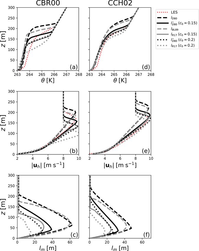
546 F. Lemarié et al.: Development of a two-way coupled ocean-wave model
of the ABL1d model in the NEMO framework. In Sects. 4 built on a simplified version of the original system of equa-
and 5 numerical results obtained for some atmosphere-only tions. In the present study we consider this latter approach,
simplified test cases available in the literature and for a cou- in the spirit of Giordani et al. (2005), who derived a sim-
pled NEMO-ABL1d simulation in a global configuration are plified oceanic model by degenerating the primitive equation
shown. Finally, our conclusions and perspectives are summa- system and prescribing geostrophic currents into the momen-
rized and discussed in Sect. 6. tum equation in substitution of the horizontal pressure gradi-
ent. In this model, a simple 1D oceanic mixed layer is three-
dimensionalized via advective terms to couple the vertical
2 Model equations columns with each other. The idea here is to translate this
idea to the MABL context. In the rest of this section we de-
In this section we first provide some basic elements on model
scribe the continuous formulation of our simplified MABL
reduction to motivate our approach and mention possible al-
model which will be referred to as ABL1d.
ternatives (Sect. 2.1). Then we detail the continuous formula-
tion of the ABL1d model and discuss the assumptions made. 2.2 Formulation of a single-column approach
In particular the governing equations and necessary bound-
ary conditions are given in Sect. 2.2 and the turbulence clo- The formulation of the ABL1d model is derived under
sure scheme for the MABL in Sect. 2.3. Finally in Sect. 2.4 the following assumptions: (i) horizontal homogeneity (i.e.,
we discuss the methodology to relax the ABL1d prognostic ∂x · = ∂y · = 0); (ii) the atmosphere in the computational do-
quantities toward large-scale data. main being transparent (i.e., ∂z I = 0 with I the radiative
flux) meaning that cloud physics is ignored and solar ra-
2.1 Motivations and proposed approach diation and precipitations at the air–sea interface are spec-
ified as usual from observations (e.g., Large and Yeager,
Global oceanic models can be run at higher resolution than
2009); (iii) vertical advection being neglected. Such assump-
global atmospheric models because of their affordable com-
tions prevent the model from prognostically accounting for
putational cost. From an oceanic perspective, we generally
the SST-induced adjustment of the atmospheric horizontal
simulate at high resolution (in space and time) ocean fields
pressure gradient and for horizontal advective processes as-
φ oce
HR (x, y, z, t) over a time interval t ∈ [0, T ] over which only sociated with a higher resolution boundary condition at the
large-scale atmospheric data φ atm LS (x, y, z, t) are known from air–sea interface. The focus here is on the proper represen-
the integration of a model Matm using lower-resolution sur-
tation of the modulation of the MABL turbulent mixing by
face oceanic data φ oceLS (x, y, z = 0, t) to compute its surface the air–sea feedback, which is thought to be the main cou-
boundary conditions, namely
pling mechanism at the characteristic scales of the oceanic
φ atm oce mesoscales impacting φ atm (z = 10 m, t) and hence air–sea
LS (x, y, z, t) = Matm (φ LS (x, y, z = 0, t)), t ∈ [0, T ].
fluxes. This mechanism is expected to explain most of the
Instead of directly using φ atmLS (x, y, z = 10 m, t) to con- eddy-scale wind–SST and wind–current interactions and is
strain the oceanic model as in the ASL forcing strategy, our key to properly downscaling large-scale atmospheric data
objective is to estimate (without running the full atmospheric produced by a coarse-resolution GCM to the oceanic resolu-
model again) the correction to the 10 m large-scale atmo- tion. At a given location in space, the ABL1d model for the
spheric data associated both with the fine resolution in the Reynolds-averaged profiles of horizontal velocities uh (z, t),
oceanic surface fields and with the two-way air–sea coupling. potential temperature θ (z, t), and specific humidity q(z, t),
Somehow we aim to find a methodology to get a cheap esti- given a suitable initial condition, is
atm
mate eφ HR (x, y, z = 10 m, t) of the solution that would have
∂t uh = −f k × uh + ∂z (Km ∂z uh ) + RLS
been obtained using a coupling of Matm and the oceanic
∂t θ = ∂z (Ks ∂z θ ) + λs (θLS − θ ) (1)
model at high resolution. To do so we could imagine sev-
∂t q = ∂z (Ks ∂z q) + λs (qLS − q)
Matm
eral approaches: (i) estimate ∂∂φ oce (i.e., the derivatives of
LS
the atmospheric solution with respect to the oceanic param- for the height z between a lower boundary zsfc and an upper
eters) via sensitivity analysis which would require to have boundary ztop , which will be considered horizontally con-
the possibility to operate Matm ; (ii) build a surrogate model stant because only the ocean and sea-ice-covered areas are
via learning strategies which would require a huge amount of interest. In Eq. (1), k = (0, 0, 1)t is a vertical unit vector,
of data and computing time; (iii) select the feedback loops f is the Coriolis parameter, Km and Ks are the eddy diffu-
of interest and define a simplified model to mimic the un- sivity for momentum and scalars respectively, the subscript
derlying physical mechanisms. Following the terminology LS is used to characterize large-scale quantities known a pri-
of Razavi et al. (2012), the first two approaches enter the ori, λs (z, t) is the inverse of a relaxation timescale, and RLS
class of statistical or empirical data-driven models emulating denotes a large-scale forcing for the momentum equation.
the original model responses while the third one enters the RLS can either represent a forcing by geostrophic winds uG
class of low-fidelity physically based surrogates which are (i.e., RLS = f k×uG ) or equivalently by a horizontal pressure
Geosci. Model Dev., 14, 543–572, 2021 https://doi.org/10.5194/gmd-14-543-2021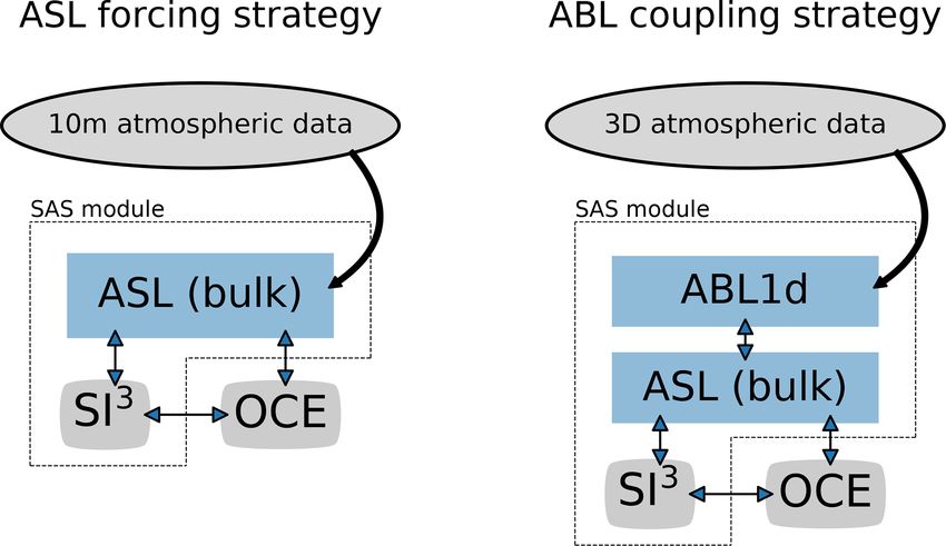
F. Lemarié et al.: Development of a two-way coupled ocean-wave model                                                                547

gradient (i.e., RLS = ρ1a ∇ h p     ) combined with a standard        Sect. 5). Note that for an ASL forcing strategy uh (zsfc )
                                 LS
Newtonian relaxation (i.e., RLS = λm (uLS −uh )). Because of          and φ(zsfc ) in Eq. (3) would be equal to uLS (z = 10 m)
the simplifications made to derive the ABL1d model the RLS            and φLS (z = 10 m) respectively, while in the ABL coupling
term and a nonzero λs are necessary to prevent the prognos-           strategy those variables are provided prognostically by
tic variables from drifting very far away from the large-scale        an ABL1d model. As far as the boundary conditions at
values used to “guide” the model. By itself a relaxation term         z = ztop are concerned, Dirichlet boundary conditions
does not directly represent any real physical process, but the        uh (ztop ) = uLS (ztop ) and φ(ztop ) = φLS (ztop ) are prescribed.
rationale is that it accounts for the influence of large-scale        Model (1) is a first step before evolving toward a more
three-dimensional circulation processes not explicitly repre-         advanced surrogate model including horizontal advection
sented in a simple 1D model. Note that this methodology               and fine-scale pressure gradients in the future. A particular
is currently used to evaluate GCM parameterizations in 1D             focus of the present study is on the appropriate choice of a
column models. Once the turbulent mixing and the Coriolis             closure scheme to diagnose the eddy diffusivities Km and
term have been computed to provide a provisional prediction           Ks . This is a key step to properly represent the downward
φ n+1,? at time n+1 for any ABL1d prognostic variable φ, the          mixing process.
relaxation term provides a weighting between this prediction
and the large-scale quantities:                                       2.3   Turbulence closure scheme

φ n+1 = 1tλ φLS + (1 − 1tλ)φ n+1,? ,                           (2)    This subsection describes the turbulence scheme used to
                                                                      compute the eddy diffusivity for momentum and scalars.
with 1t the increment of the temporal discretization. Above           Those eddy diffusivities are responsible for a vertical mixing
the boundary layer, the ABL1d formulation is unable to prop-          of atmospheric variables due to turbulent processes. The tur-
erly represent the physics; therefore the λ parameter should          bulence scheme we have implemented in our ABL1d model
be large, while in the first tens of meters near the surface          is very similar to the so-called CBR-1d scheme of Cuxart
we expect the ABL1d model to accurately represent the in-             et al. (2000), which is used operationally at Meteo France
teraction with the fine-resolution oceanic state, and thus the        (Bazile et al., 2012). We chose to recode the parameteri-
relaxation toward φLS should be small. The exact form of the          zation from scratch for several reasons: computational ef-
λs and λm coefficients is discussed later in Sect. 2.4. Note          ficiency, consistency with the NEMO coding rules, use of
that because of the relaxation term, three-dimensional
                                                         atmo-      a geopotential vertical coordinate, and flexibility to add el-
                                                  1                   ements specific to the marine atmospheric boundary layer.
spheric data for uLS , θLS , qLS , and possibly ρa ∇ h p     sam-
                                                          LS          CBR-1d is a one-equation turbulence closure model based
pled between zsfc and ztop must be provided to the oceanic
model instead of the two-dimensional data (usually at 10 m)           on a prognostic TKE and a diagnostic computation of ap-
necessary for an ASL forcing strategy. Since the ABL1d                propriate length scales. The prognostic equation for the TKE
                                                                      e = 21 u0 u0 + v 0 v 0 + w0 w0 (with h·i the Reynolds aver-

model does not include any representation of radiative pro-
cesses and microphysics, the radiative fluxes and precipita-          aging operator) is
tion at the air–sea interface are similar to the one provided for                              g
a standard uncoupled oceanic simulation. The model requires           ∂t e = − u0h w0 · ∂z huh i +  w 0 θv0
                                                                                              θvref
boundary conditions for the vertical mixing terms which are
                                                                                        1 0 0
computed via a standard bulk formulation:                                − ∂z e 0 w 0 +    p w − ε,                                  (5)
                                                                                        ρa
Km ∂z uh |z=zsfc = CD kuh (zsfc ) − uoce k(uh (zsfc ) − uoce ), (3)
                                                                      where horizontal terms and vertical advection are neglected,
Ks ∂z φ|z=zsfc = Cφ kuh (zsfc ) − uoce k(φ(zsfc ) − φoce ),    (4)
                                                                      as usually done in mesoscale atmospheric models. Here θv is
  with φ = θ, q.                                                      the virtual potential temperature, ρa is atmospheric density,
                                                                      and ε is a dissipation term. In order to express the evolution
   For the sake of consistency, it is preferable to use a
                                                                      of e in terms of Reynolds-averaged atmospheric variables we
bulk formulation as close as possible to the one used to
                                                                      consider the standard closure assumptions for the first order
compute the three-dimensional large-scale atmospheric
                                                                      turbulent fluxes (Cuxart et al., 2000) to obtain the classical
data φ atm
       LS . Because in the present study the plan is to use           TKE prognostic equation
a large-scale forcing from ECMWF reanalysis products,
we use the IFS (Integrated Forecasting System: https:                                                                    cε 3/2
//www.ecmwf.int/en/forecasts/documentation-and-support/               ∂t e = Km k∂z huh i k2 − Ks N 2 + ∂z (Ke ∂z e) −      e ,      (6)
                                                                                                                         lε
changes-ecmwf-model/ifs-documentation, last access:
20 January 2021) bulk formulation such as implemented                 where lε is a dissipative length scale, c a constant, and N 2
in the AeroBulk (https://brodeau.github.io/aerobulk/, last            is the moist Brunt–Väisälä frequency computed as N 2 =
access: 20 January 2021) package (Brodeau et al., 2017)               (g/θvref ) (∂z hθ i + 0.608 ∂z (hθ i hqi)) with θvref = 288 K. The
to compute CD , Cθ , and Cq in realistic simulations (see             eddy diffusivities for momentum Km , TKE Ke , and scalars

https://doi.org/10.5194/gmd-14-543-2021                                                     Geosci. Model Dev., 14, 543–572, 2021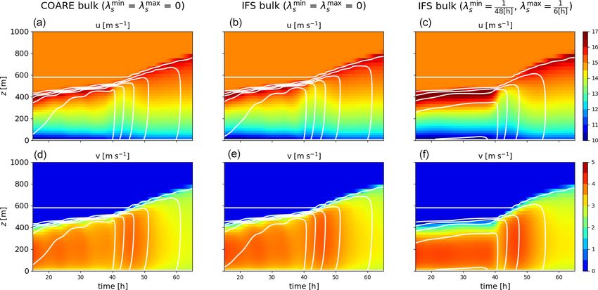
548                                                     F. Lemarié et al.: Development of a two-way coupled ocean-wave model

Ks all depend on e and on a mixing length scale lm :                 algorithm. The way esfc and Lsfc are obtained is detailed in
                                      √                              Appendix A.
(Km , Ks , Ke ) = (Cm , Cs φz , Ce )lm e,                               Our current implementation of boundary layer subgrid
                                                                     processes is an eddy-diffusivity approach which does not in-
with (Cm , Cs , Ce ) a triplet of constants and φz a stability       clude any explicit representation of boundary-layer convec-
function proportional to the inverse of a turbulent Prandtl          tive structures. This could be done via a mass-flux repre-
number, given by                                                     sentation (e.g., Hourdin et al., 2002; Soares et al., 2004) or
               n                         o−1                       the introduction of a countergradient term (e.g., Troen and
φz (z) = 1 + max C1 lm lε N 2 /e, −0.5455      .                     Mahrt, 1986). This point is left for future developments of
                                                                     the ABL1d model.
The φz function is bounded not to exceed φzmax = 2.2 as done
in the Arpege model of Meteo France (e.g., Bazile et al.,            2.4   Processing of large-scale forcing and Newtonian
2012). Assuming that the minimum of φz p       is attained in the          relaxation
linearly stratified limit (i.e., for lm = lε = 2e/N 2 ), values
of the maximum Prandtl number Prt = Cm /(Cs φz ) are given           As mentioned earlier, the ABL1d model (1) requires three-
in Table 1. Constant values for Cm , Cs , Ce , cε , and C1 can be    dimensional (x, y, z) large-scale atmospheric variables φ atmLS ,
determined from different methods, leading to nearly similar         while existing uncoupled oceanic forcing strategies require
values. The traditional way is to use the inertial–convective        only two-dimensional (x, y) atmospheric variables. This is
subrange theory of locally isotropic turbulence (Lilly, 1967;        a difficulty for efficiency reasons since it substantially in-
Deardorff, 1974). Another way relies on a theoretical turbu-         creases the number of I/Os but also for practical reasons
lence model partly based on renormalization group methods            because it requires the development of a dedicated tool to
(see Cheng et al., 2002). For the present study, the sets pro-       extract large-scale atmospheric data and interpolate them
posed by Cuxart et al. (2000) and Cheng et al. (2002) will           on prescribed geopotential heights from their native verti-
be considered (Table 1). A major difference between the two          cal grid, which can be either pressure based or arbitrary La-
sets concerns the value of Cm . This difference is explained         grangian Eulerian. Such tools have been developed specifi-
by a reevaluation of the energy redistribution among velocity        cally to work with ERA-Interim, ERA5, and operational IFS
components by pressure fluctuations, whose magnitude is as-          datasets and are described in Appendix B.
sumed to be proportional to the degree of energy anisotropy             Beyond the particular values of φ atm
                                                                                                           LS , the form of the relax-
as initially introduced by Rotta (1951). Note that the con-          ation timescale has a great impact on model solutions. The
stant set of Cheng et al. (2002) is now used by default in both      vertical profile for the λm and λs coefficients in Eq. (1) is
research and operational Meteo France models.                        chosen to nudge strongly above the MABL and moderately
   The Dirichlet boundary condition for TKE applied at the           in the MABL with a smooth transition between its minimum
top z = ztop is e(z = ztop ) = emin = 10−6 m2 s−2 and at the         and maximum value to avoid large vertical gradients in λm
bottom z = zsfc we have                                              and λs , which would result in artificially large vertical gradi-
                                                                     ents in atmospheric variables. In practice the λm (z) and λs (z)
                       u2
e(z = zsfc ) = esfc = √ ? + 0.2w?2 ,                           (7)   functions depend on the following parameters:
                       Cm cε

with u? and w? the friction and convective velocities given by          – (λmax    min         max min
                                                                              m , λm ) and (λs , λs ), which define the maxi-
the bulk formulation. The value for emin has been chosen em-              mum and minimum of the nudging coefficient for mo-
pirically as well as background values Km  min = 10−4 m2 s−1              mentum and scalars respectively. Following Eq. (2), a
       min     −5 2 −1                                                    guideline to set reasonable values for those parameter
and Ks = 10 m s for eddy diffusivities.
   The minimum value for lm is simply set as lmmin =     m
                                                         √
                                                           K min
                                                               .          values would be to make sure that 1tλmax   s   ≈ 1 (i.e.,
                                                      Cm emin
                                                                          the large-scale value is imposed above the boundary
There are multiple options to compute the mixing lengths lm
                                                                          layer) and choose λmin s   based on the typical adjust-
and lε (this point will be discussed later in Sect. 3.2.2), but
                                                                          ment timescale of the ABL to surface perturbations.
all options have identical boundary conditions lm (z = ztop ) =
 min and                                                                  Broadly speaking the ABL can be defined as the re-
lm
                                                                          gion that responds to surface forcings with a timescale
                            (Cm cε )1/4                                   of about an hour (e.g., LeMone et al., 2019). In the re-
lm (z = zsfc ) = Lsfc = κ               (zsfc + z0 ).          (8)        alistic numerical experiments shown in Sect. 5, we used
                               Cm                                                    1
                                                                          λmin
                                                                            s   = 90[min] , which, for an oceanic dynamical time
   The value of Lsfc results from the similarity theory in the            step 1t = 1080 s, would lead to 1tλmins   = 0.2. (i.e., the
neutrally stratified surface layer (Sect. 4.1 in Redelsperger             boundary layer values are the result of a weighting with
et al., 2001, and Appendix A). In Eq. (8), κ is the von Karman            a weight 0.8 for the ABL1d prediction and 0.2 for the
constant and z0 a roughness length computed within the bulk               large-scale value).

Geosci. Model Dev., 14, 543–572, 2021                                                  https://doi.org/10.5194/gmd-14-543-2021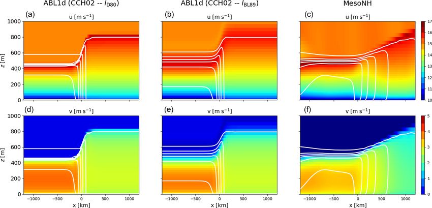
F. Lemarié et al.: Development of a two-way coupled ocean-wave model 549
Table 1. Set of turbulence scheme constants from Cuxart et al. (2000) and Cheng et al. (2002). P rt = Cm /(Cs φz ) is the turbulent Prandtl
number.
Cm Cs Ce cε C1 P rtmin P rtmax min
lm
Cuxart et al. (2000) (CBR00) 0.0667 0.1667 0.4 0.7 0.139 0.182 0.511 1.5 m
Cheng et al. (2002) (CCH02) 0.126 0.143 0.34 0.845 0.143 0.182 0.515 0.79 m
– (βmin , βmax ), which defines the extent of the transi- methods used and how this model is included in the NEMO
tion zone separating the maximum and minimum of the modeling framework. In particular, the discretization of the
nudging coefficient Coriolis term and of the TKE Eq. (6) and associated mixing
We considered the following general form for λs (z) and lengths are described in Sect. 3.1 and 3.2 respectively. De-
λm (z), with hbl the boundary layer height whose value tails about the practical implementation in NEMO are given
is diagnosed using an integral Richardson number criteria in Sect. 3.3 for the coupling aspects and 3.4 for the computa-
(Sect. 3.2 and 3.3 in Lemarié et al., 2012) with a critical value tional aspects. The ABL1d model (1) is discretized in time
equal to C1 : with an Euler backward scheme for the vertical diffusion
min terms, semi-implicitly for the Coriolis term, and explicitly
λs , m z ≤ βmin hbl , for the relaxation term, which means that the model is sta-
P3 z
λs (z) = m=0 αm hbl , z ∈]βmin hbl ; βmax hbl [, (9) ble as long as λs 1t ≤ 1. The variables are defined on a non-
max
λs , z ≥ βmax hbl , staggered grid in the horizontal (a.k.a Arakawa A-grid). Be-
cause we consider a computational domain exclusively over
where four αm coefficients are necessary to guarantee the
water or sea ice, topography is not considered and vertical
continuity of λs (z) and its derivative ∂z λs at z = βmin hbl and
levels are flat and fixed in time which, among other things,
z = βmax hbl . We easily find
allows the large-scale data φLS to be interpolated on the ver-
2 λmax +(β
(3βmax −βmin )βmin 2 min
s max −3βmin )βmax λs tical grid offline. The position of the various quantities intro-
α0 = (βmax −βmin )3
,
6β β (λ −λ ) max min duced so far on the computational grid is given in Fig. 2.
α1 = − max(β min−βs )3 s ,
max min
(β +β )(λmax −λmin ) 3.1 Coriolis term treatment
α2 = 3 max (β min−β s )3 s ,
max min
2(λmax −λmin )
α3 = − (β s −β s )3 . Since in our implementation the horizontal velocity com-
max min
ponents are collocated, the discretization of the Coriolis
The value of hbl is bounded beforehand to guarantee that at term is straightforward and is energetically neutral. In the
least 3 grid points are such that z ≤ βmin hbl and z ≥ βmax hbl . event the ABL1d is integrated with a time step much larger
A typical profile of the λs (z) is shown in Fig. 1a. than the oceanic time step, specific care must be given to
When the model is forced by the large-scale pressure gra- the stability of the Coriolis term time stepping. A semi-
dient (or the geostrophic winds), the parameter λm (z) should implicit scheme
with weighting parameter γ reads uhn+1,? =
be theoretically zero at high and middle latitudes. However,
−(f 1t)k × (1 − γ )unh + γ un+1,?
h , where the exponent ?
for the equatorial region, a Newtonian relaxation toward the
large-scale winds should be maintained. To do so, the co- is used here to emphasize that un+1,?
h is a temporary value
efficient λm (z) is multiplied by a coefficient req , which is a at time n + 1 before vertical diffusion and Newtonian relax-
function of the Coriolis parameter f . The req coefficient is ation are applied. For a given grid cell with index (i, j ), the
equal to zero for large values of |f | and increases to 1 when semi-implicit scheme can be written in a more compact way
approaching the Equator. The following form satisfies those as
constraints (see also Fig. 1b):
(1 − γ (1 − γ )(fi,j 1t)2 )uni,j + (fi,j 1t)vi,j
n
π f − fmax 6
un+1,?
i,j = ,
req (f ) = sin , 1 + (fi,j 1t)2 γ 2
2 fmax n − (f 1t)un
n+1,?
(1 − γ (1 − γ )(fi,j 1t)2 )vi,j i,j i,j
2π vi,j = .
fmax = s−1 . (10) 1 + (fi,j 1t)2 γ 2
12 × 3600
The
r associated amplification factor modulus is |Acor | =
3 Numerical discretization and implementation within 1+(1−γ )2 (f 1t)2
1+γ 2 (f 1t)2
meaning that unconditional stability is ob-
NEMO
tained as long as γ ≥ 1/2. For the numerical results obtained
We have introduced so far the continuous formulation of the below in Sects. 4 and 5 we used γ = 0.55, which is deliber-
ABL1d model. In this section we describe the discretization ately slightly dissipative.
https://doi.org/10.5194/gmd-14-543-2021 Geosci. Model Dev., 14, 543–572, 2021550 F. Lemarié et al.: Development of a two-way coupled ocean-wave model
Figure 1. (a) Typical profile of the nudging coefficient λs (z) with respect to the parameters λmax min
s , λs , βmin , βmax , hbl . (b) Equatorial
restoring function req with respect to the Coriolis frequency f .
Figure 2. Vertical grid variable arrangements and important notations.
3.2 Discretization of TKE equation where the last term can be seen as a damping term. For
ODEs like Eq. (11) it can be shown that for an initial condi-
In Sect. 2.3 we have presented the continuous formulation tion e(0) ≥ 0 and S(uh , N 2 ) ≥ 0, the solution e(t) keeps the
of the TKE-based turbulence closure of the ABL1d model. same sign as e(0) whatever the sign of the damping coeffi-
In the following we describe how the positivity of TKE cient D(e, t). Assuming that S(uh , N 2 ) and D(e, t) are pos-
can be preserved and how the mixing lengths lm and lε are itive, a backward Euler discretization of the damping term
computed. We provide a substantial discussion on the lat- n +1tS(u ,N 2 )
in Eq. (11) would lead to en+1 = e 1+1tD(e,t) h
, which pre-
ter aspect because numerical results are very sensitive to the
choices made. serves positivity since for e ≥ 0 we obtain en+1 ≥ 0. How-
n
ever, there is no guarantee that the forcing term S(uh , N 2 ) is
3.2.1 TKE positivity preservation positive, in particular when the shear is weak and the strati-
fication is large. When S(uh , N 2 ) is negative a specific treat-
The TKE equation is discretized using a backward Euler ment (known as the “Patankar trick”; see Deleersnijder et al.,
scheme in time with a linearization of the dissipation term 1997; Burchard, 2002b) is required. In the event of a negative
cε 3/2 cε √ n n+1 S(uh , N 2 ), the idea is to move the buoyancy term from S to
lε e , which is discretized as lε e e . However, such
discretization is not unconditionally positivity-preserving for D after dividing it by en , such that S(uh , N 2 ) = Km k∂z uh k2
√ 2
TKE, which could give rise to unphysical solutions (e.g., is now strictly positive and D(e, t) = clεε en + Ks Nen . Such
Burchard, 2002b). Ignoring the diffusion term, the TKE a procedure is a sufficient condition to preserve the positiv-
prognostic Eq. (6) can be written as an ordinary differential ity of the TKE without ad hoc clipping of negative values.
equation (ODE) of the form Moreover our discretization of the shear and buoyancy terms
in the TKE equation is done in an energetically consistent
∂t e = S(uh , N 2 ) − D(e, t) e, with S(uh , N 2 ) = way following Burchard (2002a).
cε √ n
Km k∂z uh k2 − Kt N 2 , D(e, t) = e , (11)
lε
Geosci. Model Dev., 14, 543–572, 2021 https://doi.org/10.5194/gmd-14-543-2021F. Lemarié et al.: Development of a two-way coupled ocean-wave model 551
3.2.2 Mixing length computation ldwn = lD80 . The resulting length scales are then limited
not only by the distance to the surface and to the top but
Another challenging task when implementing a TKE scheme also by the distance to a strongly stratified portion of
is the discretization of the mixing lengths. As mentioned ear- the air column. This limitation amounts to control of the
lier, four different discretizations of lm (lε ) have been coded. vertical gradients of lup (z) and ldwn (z) such that they are
All discretizations consider the boundary conditions given in not larger than the variations of altitude. The resulting
Eq. (8). The values of lm and lε are traditionally computed mixing length will be simply referred to as lD80 . Note
from two intermediate length scales lup and ldwn , which re- that the Taylor expansion of the integral in Eq. (13) is
spectively correspond to the maximum upward and down-
z+l
Z up
ward displacement of a parcel of air with a given initial ki- dN 2 3
2
N 2 (z)lup
2
dz lup 4
netic energy. Once lup and ldwn have been estimated by one N (s)(s − z)ds ≈ + + O(lup ),
2 3
of the methods described below, the dissipative and mixing z
length scales lm and lε are computed as
which shows that the lD80 mixing length is an approxi-
1 a mation of lBL89 , which is obtained by retaining only the
1 a 1
a
lm = lup + ldwn , (12a) leading order term in the Taylor expansion.
2
lε = min lup , ldwn , (12b) 3. Rodier et al. (2017) length scale. Recently, Rodier et al.
(2017) proposed a modification of the Bougeault and
where a ≈ − 32 for CBR00 and a ≈ − 76 for CCH02 (see Ap- Lacarrère (1989) mixing length. This modification turns
pendix A). The impact of the weighting between lup and ldwn out to improve results for stably stratified boundary lay-
to compute lm can be significant for idealized experiments ers typical of areas covered by ice. They propose to add
like the ones presented in Sect. 4.2 but for more realistic a shear-related term to Eq. (13) such that the definition
cases results are weakly sensitive and equivalent
p to the ones of lup and ldwn becomes
obtained with the simpler weighting lm = lup ldwn . z+l
Z up
In the following we provide the continuous form of the h p i
N 2 (s)(s − z) + c0 e(s)k∂s uh k ds = e(z),
various ways to compute lup and ldwn implemented in the
z
ABL1d model. The discretization aspects are detailed in Ap-
Zz h
pendix C. p i
N 2 (s)(z − s) + c0 e(s)k∂s uh k ds = e(z), (14)
1. Bougeault and Lacarrère (1989) length scale. A clas- z−ldwn
sical approach in atmospheric models is the use of the
where√c0 is a parameter whose value should be smaller
Bougeault and Lacarrère (1989) mixing length (see also
than Cm /cε . The value of c0 will be chosen based on
Bougeault and André, 1986) which defines lup and ldwn
numerical experiments presented in Sect. 4. In the fol-
as
lowing this mixing length will be referred to as lR17 .
z+l
Z up 4. A local buoyancy- and shear-based length scale. For the
N 2 (s)(s − z)ds = e(z), sake of computational efficiency, we have derived a lo-
z cal version of the Rodier et al. (2017) length scale which
Zz is original to the present paper. Under the assumption
N 2 (s)(z − s)ds = e(z). (13) that lup (ldwn ) is small compared to the spatial varia-
tions of N 2 , e, and k∂z uh k, we end up with the following
z−ldwn
second-order equation for lup :
By construction such mixing lengths are bounded by the N 2 (z) 2 p
distance to the bottom and the top of the computational lup + c0 e(z)k∂z uh klup = e(z),
domain. It is worth noting that for constant values of 2
l2 N 2 l2 N 2 whose unique positive solution is
N 2 , Eq. (13) gives up2 = e(z) and dwn2 = e(z) re- √
spectively, which is equivalent to the Deardorff (1980) ? 2 e(z)
length scale. In the remainder we will note lBL89 , the lD80 (z) = q .
mixing length obtained from Eq. (13). c0 k∂z uh k + c02 k∂z uh k2 + 2N 2 (z)
?
We easily find that lD80 = lD80 for k∂z uh k = 0, and
2. Adaptation of NEMO’s length scale. The standard √
NEMO algorithm (Sect. 10.1.3 in Madec, 2012) is sim- ?
lD80 = c0 k∂e(z)
z uh k
for N 2 = 0, which is consistent with the
ple and efficient compared to Eq. (13). This algorithm shear-based length scale of Wilson and Venayagamoor-
is ?
p based on the Deardorff (1980) length scale lD80 = thy (2015). Once lD80 has been computed we apply the
2e(z)/N 2 . lup and ldwn are first initialized to lup = same algorithmic approach as in the lD80 case.
https://doi.org/10.5194/gmd-14-543-2021 Geosci. Model Dev., 14, 543–572, 2021552 F. Lemarié et al.: Development of a two-way coupled ocean-wave model
The performance of those four length scales for various amounts to consider an Pice surface temperature averaged over
physical flows is discussed in Sect. 4. all categories T ice = nl=1cat
al Tlice for the computation of ice–
atmosphere turbulent fluxes (T ice also enters in the compu-
3.3 Coupling with ocean and sea ice tation of qice ). Noting Foce the fraction of open water (lead),
the boundary condition (15) and (16) are modified in
For the practical implementation of the ABL coupling strat-
egy within a global oceanic model, a proper coupling method Km ∂z uh |n+1 n
uoce k(un+1
z=zsfc = Foce CD kuh (zsfc ) −e uoce )
h (zsfc ) −e
is required for stability and consistency purposes (e.g., Bel-
jaars et al., 2017; Renault et al., 2019a), and the ABL1d must
ice n
+ (1 − Foce )CD uice k(un+1
kuh (zsfc ) −e h (zsfc ) −e uice ),
have the ability to handle grid cells partially covered by sea Ks ∂z φ|n+1 n
z=z = Foce Cφ ku (zsfc ) −e
sfc h uoce k(φ n+1 (zsfc ) − φ
eoce )
ice. For the coupling strategy, a so-called implicit flux cou-
uice k(φ n+1 (zsfc ) − φ
+ (1 − Foce )Cφice kunh (zsfc ) −e eice ).
pling which is unconditionally stable (Appendix B in Bel-
jaars et al., 2017) and asymptotically consistent for 1t → 0 Because the dynamics of sea ice is computed before the ther-
(Renault et al., 2019a) is used. Because vertical diffusion in modynamics (see Fig. 1 in Rousset et al., 2015), the ABL1d–
ABL1d is handled implicitly in time, the boundary condi- SI3 coupling follows these different steps:
tions (Eqs. 3 and 4) should be provided at time n+1. The im-
plicit flux coupling amounts to discretize the boundary con- 1. compute surface fluxes over ice and ocean and integrate
ditions Eqs. (3) and (4) as the ABL1d model for given values Focen and a n ,
l
Km ∂z uh |n+1 n
uoce k(un+1
z=zsfc = CD kuh (zsfc ) −e uoce ), (15) 2. compute the dynamics of sea ice,
h (zsfc ) −e
Ks ∂z φ|n+1
z=zsfc = Cφ kunh (zsfc ) −e
uoce k(φ n+1 (zsfc ) − φ
eoce ), (16) n and a n in F ? and a ? because of step 2,
3. update Foce l oce l
where e uoce and φ eoce are either the instantaneous values at 4. distribute the fluxes over each ice category considering
time n if NEMO and ABL1d have the same time step or an the updated values al? (Sect. 3.6 in Rousset et al., 2015)
average over the successive oceanic substeps otherwise.
5. compute the thermo-dynamics of sea ice.
Particular care has also been given to the compatibility be-
tween the ABL1d model and SI3 (Sea Ice model Integrated 3.4 Computational aspects
Initiative) the sea-ice component of NEMO. SI3 is a multi-
category model whose state variables relevant for our study As described in Maisonnave and Masson (2015), the NEMO
are the ice surface temperature Tlice with associated fractional source code is organized to separate the ocean routines on
area al (for the lth category), and the ice velocity uice (same one side and the routines responsible for the surface bound-
for all categories). Note that the values of the exchange co- ary conditions computation (including sea ice and the cou-
efficients over sea ice CDice , C ice , and C ice are different from
θ q pling interfaces) on the other side. This makes a clear sep-
their oceanic counterparts but are the same over all sea-ice aration between the standard ocean model (OCE compo-
categories. At this point there are several strategies for the nent) and the so-called surface module (SAS component).
ABL1d/SI3 coupling: As schematically described in Fig. 3, the ABL1d model has
been implemented within the SAS component, which allows
1. Run the ABL1d model over the whole ABL for each
the following useful features:
category l and then average atmospheric variables
weighted by al . – The ABL1d model can be run in standalone mode (cou-
pled or not with sea ice) with prescribed oceanic surface
2. Run a single ABL1d model with a category-averaged
fields.
surface flux. In the current version of NEMO Cθice is a
function of the averaged temperature T ice which means – The ABL1d model can be run in detached mode; i.e., the
that it is equivalent to compute a flux over each category OCE and SAS components run on potentially separate
before averaging them and to compute a single flux us- processors and computational grids communicating via
ing the averaged surface temperature, indeed the OASIS3-MCT coupling library (Craig et al., 2017).
X h i
al Cθice kuh (zsfc ) − uice k(θ (zsfc ) − Tlice ) = An other capability implemented within the NEMO mod-
l eling framework is the possibility to interpolate forcing fields
X
! on the fly. This is particularly useful for the ABL cou-
Cθice kuh (zsfc ) − uice k θ (zsfc ) − al Tlice . pling strategy since three-dimensional atmospheric data must
l be interpolated on the ABL1d computational grid. As the
current implementation of the on-the-fly interpolation only
The second option has been preferred because it is much works in the horizontal, the vertical interpolation of large-
easier to implement and more computationally efficient. It scale atmospheric data on the ABL1d vertical grid is done
Geosci. Model Dev., 14, 543–572, 2021 https://doi.org/10.5194/gmd-14-543-2021F. Lemarié et al.: Development of a two-way coupled ocean-wave model 553
reproduced using the code available at https://zenodo.org/
record/3904518 (last access: 20 January 2021) (Lemarié and
Samson, 2020), which also includes the scripts to generate
the figures. An objective of the present section is to illustrate
the type of sensitivity we can expect from the ABL1d model
and discriminate between the various options available in the
code. The experiments showed in Sect. 4.2 and 4.3 are meant
to investigate the impact of (i) the set of constant coefficients
(CBR00 vs. CCH02), (ii) the various formulations of lm and
lε among the algorithms described in Sect. 3.2.2, and (iii) the
parameter value c0 in the lR17 and lD80? mixing length com-
putation. Those experiments will allow several options to be
discarded. The ability of the remaining options to represent
Figure 3. Schematic representation of the ASL forcing strategy
the downward mixing mechanism, discussed in Sect. 1.2, is
(left) and ABL coupling strategy (right) in terms of code orga-
then evaluated in Sect. 4.4. The robustness of the results to
nization and required external data. The OCE and SI3 compo-
nents represent the oceanic and sea-ice dynamics and thermody- the bulk formulation and to the nudging coefficient is also
namics respectively while the ASL component is in charge of pro- checked. For each experiment we explicitly provide the ini-
viding boundary conditions related to atmospheric conditions. In tial and boundary conditions as well as all the necessary pa-
the NEMO computational framework the so-called surface module rameter values (see Table 2) so that the experiments can be
(SAS component), delineated by dashed line polygons, is virtually reproduced easily by other modeling groups.
separated from the OCE component, which allows SAS to be run in
standalone or detached mode (see Sect. 3.4). 4.2 Neutral turbulent Ekman layer
We first propose to investigate the simulation of a neutrally
offline. Nevertheless it means that the size of input data com- stratified atmosphere analogous to a classical turbulent Ek-
pared to an ASL forcing strategy is N times larger with N man layer. The selected case is based on the setup described
the number of vertical levels in the ABL. A possibility to im- in Andren et al. (1994). The initial conditions for this experi-
prove the efficiency for the reading of input data would be ment are not defined analytically; they are given by Table A1
to take advantage of the parallel I/O capabilities provided by in Andren et al. (1994)2 . This test case is mainly used to
the XIOS library (XML-IO-Server; Meurdesoif et al., 2016) check the adequacy of our surface boundary conditions with
which is currently used in NEMO only for writing output similarity theory and the proper calibration of the parameter
?
c0 in the lD80 and lR17 formulations of the mixing lengths. In
data. This technical development is left for future work. This
is a key aspect because, as discussed later in Appendix D, the theory, the lD80 and lBL89 mixing lengths do not support the
main source of computational overhead associated with the asymptotic limit N 2 = 0 but for the integrity of numerical re-
ABL coupling strategy is due to the time spent waiting for sults a minimum threshold Nε2 on the stratification is imposed
input files to be read. in the code. In this case the procedure to compute those mix-
ing lengths as described in Appendix C will provide identi-
cal results, namely lup = ztop − z and ldwn = z − zsfc (i.e., the
4 Atmosphere-only numerical experiments distance from the top and from the bottom of the computa-
?
tional domain). We test here the lD80 and lR17 introduced in
4.1 Sensitivity experiments and objectives
Sect. 3.2.2. The reference solution is taken from Cuxart et al.
To check the relevance of our ABL1d model for idealized (2000) (panels a and b in their Fig. 16). Results are obtained
atmospheric situations typical of the atmospheric bound- using the ABL1d model with either the CBR00 (Fig. 4a–d)
ary layer over water or sea ice, we performed a set of or the CCH02 (Fig. 4e–h) set of parameters. All experiments
single-column experiments. Each of those experiments are have been done with c0 = 0.15 and c0 = 0.2. All simulations
evaluated with benchmark large eddy simulations (LESs). are able to reproduce the overall behavior of the LES case.
Moreover, we use standardized test cases from the litera- The main outcomes are as follows:
ture to allow our results to be cross-compared with other – The best agreement is obtained when using the CCH02
well-established ABL schemes. In the following we con- ?
constants along with lD80 mixing length and c0 = 0.2.
sider a neutrally stratified (Sect. 4.2) and a stably stratified
(Sect. 4.3) case as well as a case with a transition from sta- – The results obtained for lD80 and lBL89 are identical and
ble to unstable stratification representative of an atmospheric close to the lR17 results with c0 = 0.15 (not shown).
flow over an SST front (Sect. 4.4). All ABL1d simulations 2 However, we did not find significant differences in numeri-
presented here have been performed directly within the SAS cal solutions when using the following initial conditions: uh (z, t =
component of the NEMO modeling framework and can be 0) = uG , e(z, t = 0) = emin .
https://doi.org/10.5194/gmd-14-543-2021 Geosci. Model Dev., 14, 543–572, 2021554 F. Lemarié et al.: Development of a two-way coupled ocean-wave model
Table 2. Description of the idealized experiments performed in Sect. 4. LMO is the Monin–Obukhov length.
Units Neutral case GABLS1 SST front
Time step [s] 60 10 10
Simulation time [h] 28 9 40
ztop [m] 1500 400 2000
Vertical levels – 40 64 50
Vertical resolution uniform uniform stretched (1z ∈ [20, 100] m)
Coriolis parameter [s−1 ] 10−4 1.39 × 10⁻⁴ 10−4
Brunt–Väisälä frequency [s−2 ] 0 3.47 × 10⁻⁴ 10−4
Geostrophic winds [m s−1 ] uG = (10, 0) uG = (8, 0) uG = (15, 0)
Roughness length [m] 0.1 0.1 COARE3.0 bulk
ψm = −4.8(z/LMO )
Stability functions – COARE3.0 bulk
ψs = −7.8(z/LMO )
θvref [K] – 283 288
– All simulations with the CCH02 set of parameters show when the CCH02 model constants are used. The best results
reasonable results. ?
are obtained for lD80 with c0 = 0.2 and lR17 with c0 = 0.15.
Solutions obtained with the CBR00 model constants system-
4.3 Stably stratified boundary layer (GABLS1) atically predict larger turbulent kinetic energy and mixing
lengths, resulting in large values of Ks in the first 100 m near
Within the Global Energy and Water Exchanges (GEWEX) the surface (not shown). The mismatch in terms of TKE is
atmospheric boundary layer study (GABLS), idealized cases partially explained by the difference in boundary conditions
for stable surface boundary layers have been investigated since with CBR00 constants we have esfc = 4.628 u2? while
(e.g., Cuxart et al., 2006). Such conditions are typical of areas with CCH02 constants we get esfc = 3.065 u2? from Eq. (7).
covered with sea ice. Here we consider the GABLS1 case, Note that the proper calibration of the c0 constant jointly with
whose technical description is available at http://turbulencia. the cε is the subject of several ongoing studies. Since our sim-
uib.es/gabls/gabls1d_desc.pdf (last access: 20 January 2021). ulations reproduce the known sensitivity to those parameters,
This experiment is particularly interesting as significant dif- the ABL1d model could directly benefit from new findings
ferences generally exist between solutions obtained from on that topic.
LES and single-column simulations, for example when The main outcomes are as follows:
the Bougeault and Lacarrère (1989) length scale is used
– The CCH02 set of parameters provides results of better
(e.g., Cuxart et al., 2006; Rodier et al., 2017). A large-
quality than the CBR00 constants. For the sake of sim-
scale geostrophic wind is imposed as well as a cooling
plicity, we will retain only the CCH02 parameters for
of the surface temperature θs (t) given by θs (t) = 263.5 −
the numerical results shown in the remainder.
0.25(t/3600 s). The parameter values for this test are re-
ported in Table 2 and the initial conditions are uh (z, t = 0) = – The buoyancy- and vertical-shear-based mixing lengths
uG , and ?
lR17 and lD80 are superior to the buoyancy-based mixing
lengths lD80 and lBL89 for stable boundary layers.
θ(z, t = 0) =
265 z ≤ 100 m 4.4 Winds across a midlatitude SST front
,
265 + 0.01(z − 100) otherwise
4.4.1 Setup and reference solutions
emin + 0.4(1 − z/250)3
z ≤ 250 m
e(z, t = 0) = .
emin otherwise An idealized experiment particularly relevant for the cou-
The solutions after 9 h of simulation are shown in Fig. 5 (left pling of the MABL with mesoscale oceanic eddies (and
panels) for CBR00 parameter values and in Fig. 5 (right pan- potentially submesoscale fronts) was initially suggested by
els) for CCH02 parameter values. The reference solution is Spall (2007) and then revised by Kilpatrick et al. (2014).
taken from Rodier et al. (2017) LESs. As expected, solutions More recently Ayet and Redelsperger (2019) derived an ana-
based on a mixing length ignoring the contribution from the lytical model based on a similar setup. The geometry of the
vertical shear exhibit a boundary layer that is too thick and problem is two-dimensional x–z with an SST front along the
a wind speed maximum located too high in altitude. Using a x axis:
buoyancy- and shear-based mixing length mitigates the issue
and provides very good agreement with reference solutions
Geosci. Model Dev., 14, 543–572, 2021 https://doi.org/10.5194/gmd-14-543-2021You can also read