A semi-automated procedure for the emitter-receiver geometry characterization of motor-controlled lidars
←
→
Page content transcription
If your browser does not render page correctly, please read the page content below
Atmos. Meas. Tech., 15, 1217–1231, 2022
https://doi.org/10.5194/amt-15-1217-2022
© Author(s) 2022. This work is distributed under
the Creative Commons Attribution 4.0 License.

A semi-automated procedure for the emitter–receiver geometry
characterization of motor-controlled lidars
Marco Di Paolantonio, Davide Dionisi, and Gian Luigi Liberti
Istituto di Scienze Marine, Consiglio Nazionale delle Ricerche, Rome, 00133, Italy

Correspondence: Marco Di Paolantonio (marco.dipaolantonio@artov.ismar.cnr.it)

Received: 29 July 2021 – Discussion started: 4 August 2021
Revised: 18 January 2022 – Accepted: 24 January 2022 – Published: 9 March 2022

Abstract. To correctly understand and interpret lidar-            are shown and discussed. The effectiveness of the mapping-
acquired signals and to provide high-quality data, the char-      based alignment was successfully verified by comparing the
acterization of the lidar transmitter–receiver geometry is re-    whole signal profile and the outcome of the telecover test,
quired. For example, being fundamental to correctly align         adopted in EARLINET, for a manual and a mapping-based
lidar systems, this characterization is useful to improve the     alignment. A significant signal increase and lowering of the
efficiency of the alignment procedure. In addition, some ap-      full overlap height (from 1500 m to less than 1000 m) was
plications (e.g. air quality monitoring) need to quantitatively   found. The overlap function was estimated down to 200 m
interpret the observations even in the range where the over-      and compared against the one obtained from a geometric
lap between the telescope field of view and the laser beam        model. The developed procedure also allowed estimating the
is incomplete. This is generally accomplished by correcting       absolute and relative tilt of the laser beam. The mapping ap-
for the overlap function. Within the frame of lidar-based net-    proach, even in simplified versions, can be adapted to other
works (e.g. ACTRIS/EARLINET, the Aerosol, Clouds and              lidars to characterize and align systems with non-motorized
Trace Gases Research Infrastructure/European Aerosol Re-          receiving geometry.
search Lidar Network), there is a need to define standardized
approaches to deal with lidar geometry issues. The multi-
wavelength multi-telescope Rayleigh–Mie–Raman “9-eyes”
system in Rome Tor Vergata, part of ACTRIS/EARLINET,              1   Introduction
has the capability, through computer-controlled servomotors,
to change the orientation of the laser beams and the 3D posi-     Lidar (light detection and ranging) techniques are an efficient
tion of the diaphragm of the receiving optical system around      tool to provide quantitative information about vertical prop-
the focal point of the telescopes. Taking advantage of these      erties in the atmosphere (Measures, 1984; Weitkamp, 2005).
instrumental design characteristics an original approach to       Thanks to the technological advancement of the last 20 years,
characterize the dependency of the acquired signal from the       the employment of lidar systems in sensing the Earth atmo-
system relative transmitter–receiver geometry (the mapping        sphere has rapidly grown. As an example, aerosol properties
procedure) was developed. The procedure consists in a set         are studied by spaceborne lidar observations (e.g. Winker et
of programs controlling both the signal acquisition as well       al., 2003; McGill et al., 2015; AEOLUS), by ground-based li-
as the motor movements. The approach includes solutions           dar networks (e.g. the European Aerosol Research Lidar Net-
to account for atmospheric and laser power variability likely     work, EARLINET, Pappalardo et al., 2014), and, recently, by
to occur during the mapping sessions. The paper describes         single-channel automated lidar ceilometers (e.g. Wiegner et
in detail the developed procedure and applications such as        al., 2014; Dionisi et al., 2018). In particular, the advanced
the optimization of the telescope/beam alignment and the          multi-wavelength elastic and Raman lidars, which are part of
estimation of the overlap function. The results of the map-       EARLINET, provide unsurpassed information for the charac-
ping applied to a single combination of telescope-laser beam      terization of aerosol optical properties. This network is now
                                                                  a key component of ACTRIS (the Aerosol, Clouds and Trace

Published by Copernicus Publications on behalf of the European Geosciences Union.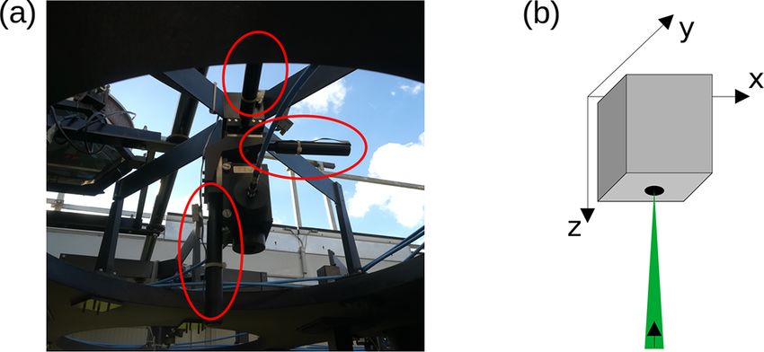
1218                                              M. Di Paolantonio et al.: A procedure for lidar geometry characterization

Gases Research Infrastructure, https://www.actris.eu/, last        geduti et al., 1999) is an old-style powerful lidar developed
access: 28 February 2022), a research infrastructure that will     in the mid-90s with the objective of monitoring the mid
coordinate the atmospheric composition observations in Eu-         and upper atmosphere (D’Aulerio et al., 2005; Campanelli
rope. Within this frame, to provide quality-assured data sets      et al., 2012; Dionisi et al., 2013a, b). To meet the EAR-
by non-standardized lidar systems, like most of those that are     LINET requirements, which the system has been part of since
part of EARLINET, one of the major efforts of this commu-          July 2016, in addition to the standard EARLINET procedure,
nity was to establish quality assurance (QA) methodologies         specific tests, based on the characteristics of the system, were
(Pappalardo et al., 2014; Wandinger et al., 2016; Freuden-         developed to characterize the RMR performance in the near
thaler et al., 2018). The expected outcome of this effort is to    range.
characterize lidar performances and check, homogenize, and            The RMR system was designed with the capability to con-
attest to the quality of the acquired data. After passing the      trol, through computer-controlled servomotors, the orienta-
QA tests, lidar raw data can then be processed by the Single       tion of the laser beams and the 3D position of the diaphragm
Calculus Chain (SCC) that allows the “automatization and           of the receiving optical system around the focal point of the
fully traceability of quality-assured aerosol optical products”    telescopes. These instrumental characteristics were exploited
(D’Amico et al., 2015). Within this frame, the characteriza-       to develop the mapping procedure: a set of semi-automated
tion of lidar transmitter–receiver geometry (e.g. Halldórsson      tools to characterize the dependency of the acquired signal
and Langerholc, 1978; Measures, 1984; Kokkalis, 2017) is           from the relative transmitter–receiver geometry.
essential to provide high-quality data.                               With respect to the existing approaches, the obtained re-
   As the main objective of EARLINET is the study of the           sults do not need any assumptions or external information
aerosol in the troposphere and boundary layer (PBL), it is         and include all artefacts due to the system that may be diffi-
important to correctly interpret the received lidar signal in      cult to account for in an analytical or numerical representa-
the lowermost range. However, bi-axial lidar systems present       tion.
an incomplete response in the near-range observational field          With the objective of optimizing the RMR observational
due to the partial overlap of the receiver field of view (FOV)     performances in the troposphere and in the PBL, the devel-
and the transmitted beam. Therefore, to use data from heights      oped procedure and two examples of applications are pre-
below the full overlap height, lidar signal profiles must be       sented in this study:
corrected for this near-field loss of signal that is the overlap
                                                                       – alignment optimization based on mapping information;
function O(R) (Wandinger and Ansmann, 2002), which de-
pends on the lidar system (e.g. Wandinger et al., 2016).               – experimental estimation of the overlap function O(R).
   Within EARLINET, the telecover test, presented by
                                                                   In Sect. 2 the relevant instrumental characteristics of the
Freudenthaler et al. (2018), is a useful and easily imple-
                                                                   RMR lidar system with a specific focus on the emitter–
mentable tool for the evaluation of the correct alignment of
                                                                   receiver geometry of the system are presented. Section 3 de-
the lidar system. This method allows identifying the lower
                                                                   scribes the developed methodology and reports examples of
height at which the lidar signal can be used to retrieve aerosol
                                                                   telescope and laser mapping. Section 4 presents the results
optical properties (i.e. the lower height of full overlap for
                                                                   obtained for two applications limited to a single wavelength
ideal lidar system); however, it cannot provide an estima-
                                                                   telescope combination. The mapping-based alignment is ver-
tion of the overlap function. In the literature various meth-
                                                                   ified through the comparison with telecover test results. The
ods were developed to compute this function both analyti-
                                                                   overlap estimation is compared to the full overlap height es-
cally and experimentally. Analytical methods (e.g. Halldórs-
                                                                   timated with the telecover test and with the predicted values
son and Langerholc, 1978; Jenness et al., 1997; Chourdakis
                                                                   using a simple geometric model based on the nominal char-
et al., 2002; Stelmaszczyk et al., 2005; Comeron et al., 2011)
                                                                   acteristic of the system as presented in Sect. 2.
require knowledge of light distribution in the laser beam
                                                                      Finally, Sect. 5 contains the summary of the developed ap-
cross section, receiver characteristics and relative inclination
                                                                   proach, the achieved main results, and short-term perspec-
of the laser beam with respect to the receiver axis. Experi-
                                                                   tives in terms of potential development. The applicability of
mental methods on the other hand make specific assumptions
                                                                   the proposed approach to other systems is also discussed.
or have special requirements based on the method: clear air
and homogeneous aerosol distribution (Sasano et al., 1979),
statistically homogeneous distribution (Tomine et al., 1989),      2    System description
extrapolation via polynomial regression (Dho et al., 1997), a
second profile with lower overlap (e.g. ceilometer, Guerrero-      The design of the multi-channel multi-telescope RMR 9-
Rascado et al., 2010; Sicard et al., 2020), or a Raman channel     eyes lidar was first presented by Congeduti et al. (1999).
with the assumption of similar receiver geometrical configu-       Since 2002 the system has been operating in the Tor Vergata
ration (Wandinger and Ansmann, 2002).                              experimental field in a semi-urban area southeast of Rome
   The multi-wavelength multi-telescope Rayleigh–Mie–              (41.8422◦ N, 12.6474◦ E; 107 m a.s.l.). Its current configura-
Raman (RMR) “9-eyes” system in Rome Tor Vergata (Con-              tion is described in detail by Dionisi et al. (2010).

Atmos. Meas. Tech., 15, 1217–1231, 2022                                             https://doi.org/10.5194/amt-15-1217-2022
M. Di Paolantonio et al.: A procedure for lidar geometry characterization 1219
Table 1. Transmitter characteristics of the RMR lidar system. telescope, fixed 0.8 mm for the others) that is in the focal
position, there is a dichroic beam-splitting optical system
Laser type Nd:YAG that separates the signals at λ < 440 nm from the ones at
Wavelength [nm] 355–532 λ > 440 nm and directs them in two different large-core op-
Nominal energy per pulse [mJ] ∼ 400 (355 nm), ∼ 200 (532 nm) tical fibres, with 0.94 mm core diameter and 0.22 numeri-
Pulse duration [ns] 7 cal aperture. In this optical system (see Fig. 3 for a detailed
Pulse repetition rate [Hz] 10 description), a one-to-one coupling of the field diaphragm
Beam diameter dL [cm] 5.0 (after the 5× beam expander)
Beam divergence 9L [mrad] 0.1 (nominal, full angle after
on the optical fibre is obtained employing a set of lenses
beam expander) (f = 20 mm): first to collimate the radiation on the dichroic
Pointing stability [mrad] ∼ 0.05 mirror and then to focus the resulting different wavelength
signals on the input face of the respective fibre. Each receiv-
ing block has been aligned on an optical bench before being
mounted on the lidar system.
Field diaphragm, dichroic beam-splitting optical system,
and SubMiniature version A (SMA) connectors for the two
optical fibre input faces are assembled in a small box sup-
plied with adjustments for lens focusing and dichroic mirror
alignment. A system of three orthogonal linear stages allows
moving each box along the x, y, and z axes by means of
computer-controlled servomotors, to find optimal alignment
and focusing positions autonomously for each telescope.
Figure 1. (a) Top view of the two 45◦ mirrors with azimuth and A total of 37 servomotors (three for each telescope and
zenith servomotors (components circled in red). (b) Schematic of two for each emitting wavelength) are present. Two models
the mirror/beam movements.
of EOTECH Testine Micrometriche Servocontrollate (TMS)
are used: the TMS-25 for the movements in the z-axis direc-
Here the relevant characteristics of the lidar system with tion of the receiving system in the telescopes and the TMS-16
an emphasis on the geometry of the emitting/receiving com- for all other movements. Table 3 reports the nominal charac-
ponents are presented. teristics of the employed servomotors. Each motor is con-
The lidar transmitter is based on a Nd:YAG laser (Con- trolled by a dedicated board. The boards can be connected
tinuum Powerlite 8010) with second (532 nm: green) and in a serial way to control more boards with a single RS-232
third (355 nm: UV) harmonic generators. The energy out- serial port. A set of three racks containing up to 14 boards is
put is optimized for the exploitation of the UV Raman scat- used to control the motors through three serial ports. Motors
tering. Backscattered radiation is collected and analysed at belonging to a given telescope or emitting mirror are grouped
four wavelengths of interest: 532 and 355 nm for the elas- in a single rack: for this reason, it is possible to control only
tic backscattering and 386.7 and 407.5 nm for Raman scat- one motor at once.
tering of N2 and H2 O molecules, respectively. The charac- Two large carbon-fibre planes are utilized to support, re-
teristics of the transmitted beam are reported in Table 1. In spectively, the telescopes (the lower ones) and the spiders
particular, it is noteworthy that the 355 and 532 nm beams holding the x–y–z motor-moved stages with the dichroic
are collimated by means of 5× beam expanders, and, then, boxes; fibreglass columns stick the two planes together. With
they are vertically projected into the atmosphere through two this architecture of the telescope-supporting frame, effects on
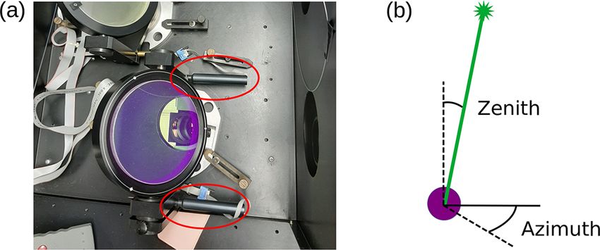
45◦ mirrors that can be azimuth- and zenith-oriented through the alignment of thermal deformations are minimized. The
computer-controlled servomotors (Fig. 1). receiving optical system with the servomotors is depicted in
The receiver is based on a multiple-telescope configura- Fig. 4.
tion allowing the sounding of a wide altitude atmospheric In the current setting, for the smallest telescope (15 cm),
interval: only the optical fibre carrying the signal return at λ > 440 nm
exits the dichroic system, as this telescope is used only for
– one single 15 cm aperture telescope for the lower layers, the elastic backscattering at 532 nm. Then, the optical fibres
bring the light from the telescopes to the photomultipliers
– one single 30 cm telescope for the middle layers, (PMTs) after passing collimating lens and interference filters
– an array of 9 × 50 cm telescopes for the upper layers that select the wavelengths of interests.
(∼ 1.7 m2 total collecting area, see Fig. 2). Currently eight acquisition channels both in photon-
counting mode as well as analogue mode are implemented;
The characteristics of the telescopes are reported in Ta- Table 4 provides an overview of the RMR channels with their
ble 2. For each of the 11 telescopes, behind the field stop associated telescopes and receiving wavelengths.
diaphragm (0.2, 0.4, 0.6, 0.8 mm diameter for the 30 cm
https://doi.org/10.5194/amt-15-1217-2022 Atmos. Meas. Tech., 15, 1217–1231, 2022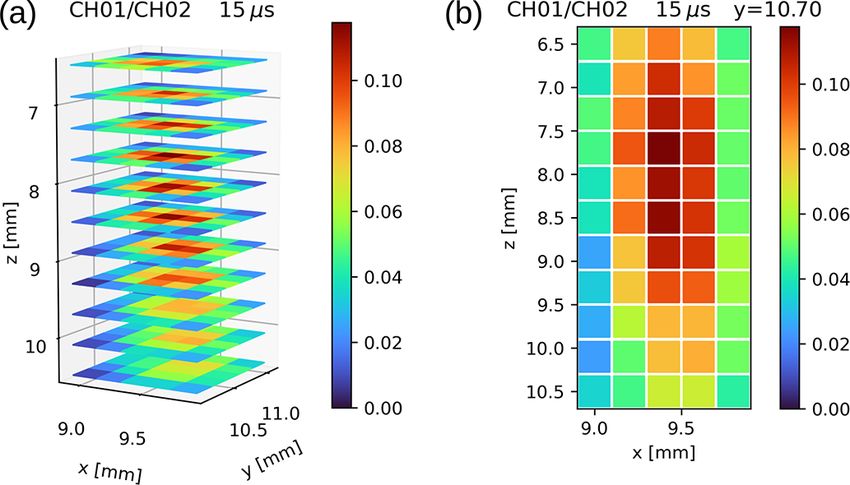
1220                                                   M. Di Paolantonio et al.: A procedure for lidar geometry characterization

Table 2. Telescope characteristics.

                                                                         Collector 1   Collector 2   Collector 3
                                                                 Nine Newtonians          Single         Single
                                Type of telescope                           array      Newtonian      Newtonian
                                Diameter [cm]                           50 (each)             30             15
                                Focal length f [cm]                          150              90             45
                                f number                                      f /3          f /3           f /3
                                FOV (full angle) 9T [mrad]                    0.5            0.9            1.8

Figure 2. (a) Top view schematic of the relative position of the laser beams (355 and 532) and the 11 telescopes. (b) Details of the emission
and low-range telescopes (15 and 30 cm).

                                                                             Figure 4. (a) Receiving optical system with the three axis servomo-
                                                                             tors (red circled components). (b) Schematic of the receiving block
                                                                             movements.

                                                                             identical vertical resolution as in the counting channels and,
                                                                             simultaneously, to improve the accuracy of the recorded data.
                                                                             Thus, in the usual operation, the vertical resolution is 75 m
                                                                             (corresponding to 0.5 µs bins) and the signals are generally
Figure 3. Schematic of the receiving block: (a) field stop diaphragm         integrated over 60 s (600 laser pulses) before recording.
(0.8 mm diameter), (b) collimation lenses (f = 20 mm), (c) dichroic             The relative emitter–receiver geometry can be modelled
beam splitter (λ = 440 nm), (d) 45◦ mirror, and (e) optical fibre con-       knowing the characteristics of emitters and receivers (Ta-
nector. Dichroic beam splitter and UV collimation lens are currently         bles 1 and 2) and the distance between the centres of each
not present in the receiving block of the 15 cm telescope.                   combination of emitter and receiver.
                                                                                Summarizing, given

   For standard measurement sessions the acquisition system                    – dcc , the distance between the centres of the laser beam
is set to acquire the photon-counting mode signals for 2000                      and the telescope,
bins with a 0.5 µs integration per bin. Samples in the ana-
logue channels are acquired at a fastest rate, with 0.05 µs                    – 9L and 9T , the divergence (full opening angle) of the
sampling rate, but they are averaged in groups of 10 to have                     laser beam and the telescope, respectively,

Atmos. Meas. Tech., 15, 1217–1231, 2022                                                        https://doi.org/10.5194/amt-15-1217-2022
M. Di Paolantonio et al.: A procedure for lidar geometry characterization                                                               1221

Table 3. Nominal characteristics of the servomotors.

                                           Range         Speed        Acceleration    Resolution   Accuracy
                                Model      [mm]        [mm s−1 ]        [mm s−2 ]          [µm]        [µm]
                                TMS-16         16             0.2               0.2            1          ±3
                                TMS-25         25             0.2               0.2            1          ±4

Table 4. Wavelengths and telescopes used for each currently imple-
mented channel.

                    355 nm    386 nm     407 nm     532 nm
       15 cm                   CH01
       30 cm        CH08       CH04       CH05         CH02
       9 × 50 cm               CH06       CH07         CH03

  – dL and dT , the beam and telescope diameter, respec-
    tively,
                                                                           Figure 5. Schematic of the overlap between the telescope FOV (red)
and assuming                                                               and the laser beam (green). Full overlap is reached inside the cone
                                                                           delimited by the dash–dotted lines. R0 and R1 heights are high-
  – parallel vertical axes (beam and telescope FOV),                       lighted by the horizontal lines.

  – aperture in the focal plane (focus at infinity),
                                                                              A more realistic theoretical estimation of the whole over-
it is possible to calculate the following geometrical charac-              lap function is possible. However, it requires accurate knowl-
teristics relevant for the description of the overlap function             edge of the real characteristics and positions of the opti-
O(R) (Stelmaszczyk et al., 2005):                                          cal parts of the system (e.g. beam shape, relative inclina-
       2dcc − dT − dL                                                      tion between the laser beam and telescope axis). The esti-
R0 =                  ,                                         (1)        mation of these parameters needs a characterization of the
         9T + 9L
                                                                           lidar emitting–receiving components that is often difficult to
                                                                           perform. The proposed approach to characterize the geome-
       2dcc + dT + dL                                                      try of the signal (Sect. 3) allows an estimation of the overlap
R1 =                  ,                                         (2)        function (Sect. 4.2).
         9T − 9L
                                                                              The following sections will focus on the characterization
where R0 is the lowermost height at which the laser beam                   of channel 1 (532 nm, 15 cm telescope). This is the channel
enters the telescope field of view and R1 is the full over-                dedicated to the PBL sensing, for which the knowledge of the
lap height (i.e. the lowermost height with O(R) = 1). As an                overlap function is fundamental. The procedure described is
example, Fig. 5 shows the case of the 15 cm telescope and                  however applicable to all the remaining laser/telescope com-
532 nm beam. These equations are equivalent to the ones cal-               binations for quality control and signal optimization.
culated from the diaphragm point of view (Halldórsson and
Langerholc, 1978; Measures, 1984) taking into account the
                                                                           3    The mapping procedure
previously stated assumptions.
   Table 5 completes the description of the geometry by re-                The mapping procedure takes advantage of the possibility
porting, for each telescope, the telescope diameter (dT ), the             of investigating the dependency of the acquired signal S(R)
field of view (9T ), and the distance from each emitting                   from the relative transmitter–receiver geometry by control-
source (dcc 532 , dcc 355 ). Based on the nominal characteris-             ling the orientation of the laser beam and the 3D position of
tics of the RMR system and the analytical model described                  the diaphragm of the receiving optical system around the fo-
above (Eqs. 1 and 2), the values of R0 and R1 have been com-               cal point of the telescopes. The procedure is based on a set
puted for all implemented combinations of emission laser                   of programs controlling both the signal acquisition as well as
wavelengths (355 and 532 nm) and telescopes. Results are                   the motor movements, and it is fully defined by setting the
reported in Table 5. It has to be noted that the full overlap              following variables:
height can be optimized by tilting properly the laser beam
with respect to the telescope axis (Kokkalis, 2017).                           – telescope/laser beam of interest

https://doi.org/10.5194/amt-15-1217-2022                                                      Atmos. Meas. Tech., 15, 1217–1231, 2022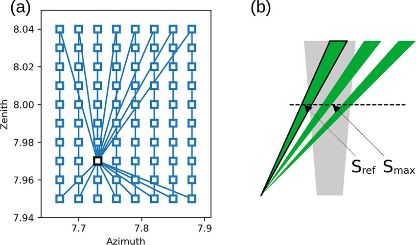
1222                                                M. Di Paolantonio et al.: A procedure for lidar geometry characterization

Table 5. Characteristics, initial (R0 ) and full (R1 ) overlap heights of the 11 telescopes for each emitted wavelength. Laser beam radius
dL = 5.0 cm and divergence 9L = 0.1 mrad were used for the calculations. The specifications of interest for this study (channel 1: 532 nm,
15 cm telescope) are highlighted in bold. NA = not available.

                  Telescope          1       2       3       4       5         6       7        8        9      10       11
                  dcc 532 [cm]   121        63      46      32      82      125      140       80      35       63      122
                  dcc 355 [cm]   124        62      25      20      66      141      138       85      56       84      137
                  dT [cm]          50       50      30      15      50       50       50       50      50       50       50
                  9T [mrad]      0.53     0.53    0.89    1.78    0.53     0.53     0.53     0.53    0.53     0.53     0.53
                  R0 532   [m]   2953    1121     576     234    1721      3079    3553     1658      237    1121     2984
                  R0 355   [m]   3047    1089     152     NA     1216      3584    3489     1816      900    1784     3458
                  R1 532   [m]   6854    4177    1610     501    5054      7038    7731     4962     2885    4177     6900
                  R1 355   [m]   6992    4131    1077     NA     4315      7777    7638     5192     3854    5146     7592

  – reference/starting position (x0 , y0 , z0 for the telescopes,
    Az0 , Zen0 for the laser beams);

  – range and regular step in each direction independently
    (i.e. number of acquisitions);

  – channels to be acquired;

  – acquisition characteristics (e.g. duration, bin size).

Defining these parameters is a trade-off between having de-
tailed and low-noise information and minimizing the signal
variability introduced by changes in the atmosphere and in
the lidar system (e.g. laser power). To minimize the atmo-
spheric variability, the mapping procedure should be prefer-
                                                                         Figure 6. Example of telescope mapping geometry in the x–y plane
ably performed in stable meteorological conditions (e.g. end             (used for the first measurement session described in this work); x
of the night). However, strategies to monitor/account for                and y relative position of the servomotors in the respective axis.
these variabilities have been implemented and will be dis-
cussed for each example of mapping reported.
   The single telescope and laser mapping are described in
detail in the following subsections.

3.1    Telescope mapping

The telescope mapping procedure controls the position of
the optical system in all three axes. This procedure is im-
plemented by performing, for a given set of z positions, a
series of acquisitions in the horizontal plane (x and y direc-
tions). Each x–y plane is scanned starting from a reference
position (x0 , y0 ) along a spiral path, in order to minimize the        Figure 7. (a) Expected radii for maximum (rd − ri ) and partial
necessary motor movements (see example in Fig. 6).                       counts (rd + ri ) in the signal map for an image of radius ri and a
   Given the relative dimension of the diaphragm and the op-             diaphragm (solid line) of radius rd for ri < rd . (b) Schematic longi-
tical fibre core and assuming a well-aligned receiving box,              tudinal view of radiation intensity near the focal plane, diaphragm
the procedure presented in this study takes into account only            in a focused (1) and in an out-of-focus (2) position.
the characterizable effect of the field stop diaphragm dis-
placement.
   Moving the diaphragm in the x–y plane on a fixed z for                that all the signal passing through the diaphragm is captured
an image of radius ri < rd , where rd is the diaphragm ra-               by the PMT. When the signal is clipped in the path between
dius, approximately constant counts are expected in a circle             the aperture and the sensor, the obtained mapping could be
of radius rd − ri and a decrease to zero counts within a ra-             asymmetric and could diverge from the expected shape. The
dius rd + ri (Fig. 7a). This of course under the assumption              resulting image could also be affected by inhomogeneities in

Atmos. Meas. Tech., 15, 1217–1231, 2022                                                     https://doi.org/10.5194/amt-15-1217-2022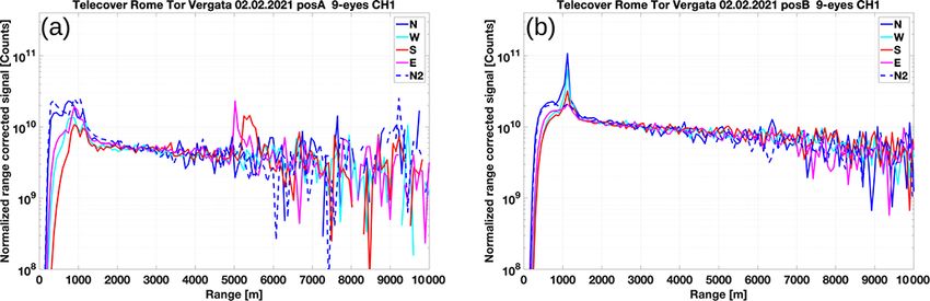
M. Di Paolantonio et al.: A procedure for lidar geometry characterization                                                         1223

Figure 8. (a) Simulated signal map for a diaphragm of radius rd = 0.4 mm and an image of radius ri = 0.2 mm. The signal is normalized by
the maximum value. (b) Result of a single-plane mapping performed with misaligned optics; here the signal (normalized by the maximum
value) is asymmetrically clipped by the optical system between the telescope and the photomultiplier.

the PMT sensitivity (Freudenthaler, 2004); the use of optical         where f is the telescope focal length and D is the geometric
fibres effectively acts as a light scrambler minimizing the im-       distance between the position x, y and the reference position
pact of this problem (Sherlock et al., 1999). Small imperfec-         xc , yc .
tions in the beam cross section, when the image is small and             As previously mentioned, a trade-off between obtaining a
well-focused, should not cause asymmetries in the resulting           reasonable signal-to-noise ratio (SNR) in the range of inter-
mapping.                                                              est and minimizing possible changes in the signals due to
   For a fixed range R in lidar-acquired profiles, when chang-        atmospheric and system variability is needed.
ing the z coordinate of the field stop/diaphragm, the image is           In order to account for atmospheric/system variability, two
expected to grow from the minimum in the focused position             approaches have been tested:
following the enlargement of the circle of confusion. If the             – If there is a channel acquiring information at the
image size is bigger than the receiving optical component                  same wavelength of the channel being mapped but
(e.g. diaphragm, optical fibre, lens), part of the signal will be          through another telescope, a normalized signal is ob-
lost but the mapping will still be symmetric (Fig. 7b).                    tained from the ratio of the profiles from the two
   From the qualitative analyses of acquired signals from a                channels. For example, the normalized signal S 0 (R) =
single telescope mapping, knowing the ideal behaviour, it is               SCH01 (R)/SCH02 (R) used for the mapping of channel 1
possible to diagnose deviations from the nominal positions                 described in the following section (Sect. 4.1) is defined
for all the optical components in the system not taken into                as the ratio of the simultaneously acquired measure-
account by the simplified model. As an example, Fig. 8 de-                 ments from channel 1 and 2 (Table 4).
picts a simulated single-plane mapping in case of good align-
ment and a real mapping showing problems with the optical                – In the absence of a suitable signal from a second chan-
alignment (i.e. signal clipping in the optical system between              nel, the signal profile from the same channel, acquired
the telescope and the photomultiplier).                                    periodically in a reference position (e.g. the position
   The information given by this type of mapping can be used               chosen with a previous alignment) during the mapping,
to accurately position the receiving optical system as shown               can be used to normalize the measurements within the
in Sect. 4. Another potential use of the information derived               interval of time between acquisitions in the reference
from the mapping is to estimate unknown characteristics of                 position. This approach is used in the laser mapping
the system.                                                                (Sects. 3.2 and 4.2); in this case the normalized signal
                                                                                                                   ref (R).
                                                                           was calculated as S 0 (R) = SCH01 (R)/SCH01
   As an example, the relative tilt between the field of view
axis and the laser beam can be computed once the centre
of the image in the focal plane (xc , yc ) is found. For high         3.2   Laser mapping
ranges, this position corresponds to a configuration with par-
                                                                      In the case of lidar systems with the capability of electron-
allel beam and field of view axes. If the measurements are
                                                                      ically controlled azimuth and zenith orientation of the laser
done at different positions of the receiving system in the hor-
                                                                      beam, an analogous procedure can be implemented, leading
izontal plane, the relative tilt angle θtilt can be calculated for
                                                                      to similar insights into the geometry of the system.
any given position (x, y) with the following formula:
                                                                         For a given telescope-laser relative geometry the over-
                                                                      lap function can be estimated through a mapping performed
          D(xc , yc , x, y)                                           varying the laser beam zenith and azimuth angle. The lower-
θtilt =                     ,                                 (3)     most range for which the overlap function can be estimated
                 f

https://doi.org/10.5194/amt-15-1217-2022                                                 Atmos. Meas. Tech., 15, 1217–1231, 2022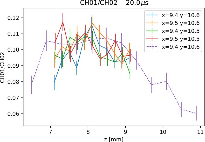
1224                                                M. Di Paolantonio et al.: A procedure for lidar geometry characterization

                                                                      tic backscatter by the 15 cm telescope (CH01). This has been
                                                                      performed in two steps:
                                                                        – a preliminary mapping with a larger range and a coarser
                                                                          step in the three dimensions to identify the sub-volume
                                                                          of optimal alignment;
                                                                        – a mapping in the sub-volume identified in the first map-
                                                                          ping, close to the optimal position and with finer reso-
                                                                          lution.

                                                                         Two steps are needed due to the time necessary to perform
                                                                      a scan with both large x–y–z range and step. The first map-
                                                                      ping could be skipped if the system was recently aligned.
Figure 9. (a) Laser mapping scan geometry, after each zenith scan a
                                                                         The two sessions were performed on 13 January 2021
measurement in the reference position (black square) is performed.
                                                                      (18:01–23:04 UTC) and on 26 January 2021 (17:02–
(b) Schematic of the telescope FOV and laser beam for different
orientations.                                                         20:01 UTC).
                                                                         Table 6 reports the characteristics of the performed map-
                                                                      ping.
depends on the characteristics of the system being required              With these settings, each acquisition for the mapping pro-
that the laser beam can be tilted to have some position with          cedure took about 38 s of which 30 s are the effective acqui-
full overlap. Moreover, in order to define an absolute maxi-          sition time and 8 s are dedicated to the data transfer and the
mum with O(R) = 1, the size of the image has to be smaller            movement of the motors that can be performed one motor at
than the diaphragm (i.e. the image is sufficiently focused).          a time.
   The scan is performed progressively, minimizing the nec-              From the results, which are depicted in Figs. 10 and 11, it
essary motor movements (Fig. 9) and the subsequent delay              is clear that the telescope in the manually optimized config-
between acquisitions. To monitor changes in the atmospheric           uration (x = 9.40 mm, y = 10.50 mm, z = 10.50 mm, high-
conditions and in the power output of the laser, an acqui-            lighted in Fig. 11a), despite being not far from the optimal
sition in a reference laser position (e.g. the setup chosen           x–y position, is highly out of focus due to its z position.
with the telescope mapping and used for routine measure-              The overall intensity of the signal in the x–y plane increases,
ments) is performed before and after each zenith swipe. This          changing the z position (Fig. 11b), as the now focused image
is highlighted in Fig. 9, where at the beginning and at the           passes through the diaphragm without being clipped. Mov-
end of each column (i.e. zenith angle swipe) the laser beam           ing further in the z axis, the signal starts again to decrease
returns to the same pair of zenith and azimuth values. Time-          (Fig. 11c). No clear asymmetries in the signal are found.
                                                      ref (R)
interpolated data acquired in the reference position SCH01            The presumed optimal position resulting from this session
are used to normalize the measurements during the mapping.            is x = 9.40 mm, y = 10.60 mm, z = 8.50 mm.
   To estimate the overlap function, for each range value R,             The slight shift of the image centre (i.e. the centre of the
the maximum (or the mean of the highest n values if the map-          area with maximum values) at different z positions is caused
ping is performed with sufficient x–y resolution) of the nor-         by incoming light rays tilted with respect to the z axis. More-
                  0
malized signal Smax   is sought. Under the previously stated          over, looking at the uppermost useful range, for x–y posi-
assumptions, this value should represent the ratio of a full          tions at the centre of the image the beam and telescope axis
                     ref
overlap signal and SCH01   affected by partial overlap. Conse-        (more precisely the FOV axis) should be approximately par-
quently, for a given range R, the overlap factor in the ref-          allel. Assuming the z axis as vertical, this information can be
erence position is 1/Smax0 . We therefore calculate the over-         used to estimate the tilt of the laser beam dividing the x–y
lap function O(R) for each R between the minimum range                shift of the centre of the image by the z displacement, result-
with useful signal and the range in which the full overlap is         ing in a tilt of ∼ 50 mrad.
reached.                                                                 The second session was performed with finer steps and
                                                                      centred around the presumed optimal position. In Fig. 12 is
                                                                      plotted the signal intensity S at different ranges and a fixed
                                                                      z coordinate. In this case, the signal has not been normal-
4     Results                                                         ized due to highly incomplete overlap of the second chan-
                                                                      nel in the low range. The atmospheric and power variability
4.1    Telescope mapping and alignment                                has been monitored qualitatively with channel-2 measure-
                                                                      ments at higher ranges. In the x–y plane, as expected, the
The objective of this telescope mapping session is to opti-           image shifts at different altitudes. No evident asymmetries
mize the alignment relative to the acquisition of 532 nm elas-        are present in the signal map.

Atmos. Meas. Tech., 15, 1217–1231, 2022                                                https://doi.org/10.5194/amt-15-1217-2022
M. Di Paolantonio et al.: A procedure for lidar geometry characterization                                                             1225

Figure 10. Overall view (a) and x–z section (b) of the results of the telescope mapping of the first session (13 January 2021) showing the
normalized signal as a function of the x–y–z positions at a chosen range (15 µs – 2250 m a.g.l.).

Figure 11. Signal mapping of the first session (13 January 2021) showing the normalized signal for three planes at different z positions and
chosen range (15 µs – 2250 m a.g.l.). The position derived from the manual alignment is highlighted by the black square.

   Through this session, a definitive and well-aligned posi-            4.2    Alignment validation
tion can be selected in the x–y plane as a trade-off between
maximizing counts in the lower range (optimizing the sig-               The selected alignment configuration was validated through
nal in the partial overlap range and lowering the full overlap          a telecover test and direct comparison of the signal profiles
height) and maintaining the beam in the telescope FOV at                in the different positions.
high ranges.                                                               The telecover test, described by Freudenthaler et
   In the z coordinate, the optimal position is selected eval-          al. (2018), is a quality assurance tool used for lidar system
uating the normalized signals at a medium range around the              misalignment diagnostic and evaluation of the full overlap
selected x and y position. As shown in Fig. 13, the curve has           range. Lidar profiles taken with different sectors of the tele-
a plateau in which the maximum value is reached (i.e. the im-           scope aperture are compared to each other. For well-designed
age is sufficiently focused and inside the diaphragm). The se-          and correctly aligned systems, the normalized signals should
lection of a position in the higher-value portion of the plateau        only show differences in the partial overlap range.
corresponds to a diaphragm position that better captures the               Measurements were carried out during a single night ses-
signal in the lowermost range (the focus shifts from infinity           sion (2 February 2021, 18:55–21:26 UTC). Progressively the
to lower ranges).                                                       following measurements were performed (see Fig. 14): a
   Based on the above considerations the derived optimal po-            telecover test in the non-optimized starting position (a), a full
sition is x = 9.45 mm, y = 10.55 mm, z = 8.30 mm.                       telescope measurement in the same position (b) and one in
   As mentioned in Sect. 3.1, measuring the angular distance            the optimized position (c), and finally a telecover test in the
between the selected position and the centre of the image at            optimized position (d). Standard acquisition times were used
high ranges (Eq. 3), the relative tilt between the telescope            (60 s), with an integration time of 10 min for each telecover
FOV axis and the laser beam is about 0.3 mrad.                          test sector or comparison profile.

https://doi.org/10.5194/amt-15-1217-2022                                                   Atmos. Meas. Tech., 15, 1217–1231, 2022
1226                                                M. Di Paolantonio et al.: A procedure for lidar geometry characterization

Table 6. Characteristics of the two telescope mapping sessions and the laser mapping session; the channels used for the procedure are
highlighted in bold.

                  Mapping type                                    Telescope             Telescope                 Laser
                                                               13 Jan 2021,           26 Jan 2021,         15 Feb 2021,
                  Time                                    18:01–23:04 UTC        17:02–20:01 UTC       18:39–19:37 UTC
                  Mapped telescope/laser beam                      4 (15 cm)             4 (15 cm)              532 nm
                  Starting/reference position
                  x, y, z/Az, Zen [mm]                    9.40, 10.60, 10.90      9.40, 10.60, 9.10           7.73, 7.97
                  Range, step for x axis/Az axis [mm]               0.8, 0.2               0.4, 0.1           0.21, 0.03
                  Range, step for y axis/Zen axis [mm]              0.8, 0.2               0.4, 0.1           0.09, 0.01
                  Range, step z axis [mm]                           4.4, 0.4               2.0, 0.2
                  Channels acquired                                1, 2, 4, 8             1, 2, 4, 8           1, 2, 4, 8
                  Single acquisition duration [s]                         20                     30                   30
                  Bin size [µs]                                          5.0                    0.5                  0.5
                  Total mapping time                              2 h 52 min            2 h 59 min               58 min

Figure 12. Signal mapping (CH01 photon-counting signal) of the second session (26 January 2021) at same z and different ranges (a: 5.0 µs
– 750 m; b: 10.0 µs – 1500 m; c: 20.0 µs – 3000 m). Here the signal is not normalized due to the lack of sufficient SNR from the second
channel in the lower range (highly incomplete overlap).

4.2.1   Profile comparison                                             ble impact of mirror imperfections and the irregular shape of
                                                                       the laser beam, this has been confirmed to be due to the di-
Figure 15a shows the direct comparison of the background               aphragm in an out-of-focus position for the z axis. This leads
subtracted signal profiles in the non-optimized starting posi-         to an image in the aperture plane with a large circle of con-
tion and in the optimized position. Higher signal is found in          fusion and non-optimal alignment of the field of view (x and
the whole optimized profile (> 50 % relative normalized dif-           y axes).
ference), confirming the successful alignment procedure and               Figure 16b depicts the results in the optimized position.
no signal loss in the high range (Fig. 15b). The negative dif-         The full overlap height is around 1000 m or less, and the rel-
ference in the lowermost range is well below the full overlap          ative difference of the signals in the partial overlap region
height (i.e. < 500 m) and can be explained considering that            has decreased. Atmospheric variability and the presence of
the large and less focused image of the non-optimized posi-            aerosol layers prevent a more precise evaluation of the over-
tion can maintain a partial overlap with the telescope FOV             lap height using the telecover QA method. As expected, less
for a wider vertical range.                                            noise is detected in all ranges due to the increased signal.

4.2.2   Telecover                                                      4.3      Laser mapping and overlap estimation

Two telecover tests were conducted: one in the non-                    Once an optimized position has been selected and verified
optimized starting position (Fig. 16a) and one in the opti-            (see Sect. 4.1 and 4.2), a laser beam mapping with the
mized position (Fig. 16b). Figure 16a shows that the height            purpose of estimating the overlap function was performed
of full overlap is higher than 1500 m, far from the expected           (15 February 2021, 18:39–19:37 UTC). The characteristics
modelled value of 501 m (see Table 5). Assuming a negligi-             of the mapping are reported in Table 6. In Fig. 17 the mapped

Atmos. Meas. Tech., 15, 1217–1231, 2022                                                   https://doi.org/10.5194/amt-15-1217-2022
M. Di Paolantonio et al.: A procedure for lidar geometry characterization 1227
Figure 15. Background subtracted counts (a) and relative difference
between the normalized signal CH01/CH02 profiles (b) in the se-
lected position (x = 9.45 mm y = 10.55 mm z = 8.30 mm) and the
Figure 13. Normalized signal at a chosen range (20 µs – 3000 m) starting one (x = 9.40 mm y = 10.50 mm z = 10.50 mm).
for different x and y positions as a function of z; data from both
mapping sessions (dashed line for the first session, solid line for the
second). A plateau is reached approximately between z = 7 mm and
z = 9 mm. Each colour corresponds to different x and y positions as form beam energy distribution (Stelmaszczyk et al., 2005)
indicated in the legend of the plot. and a Monte Carlo integration of Halldórsson and Langer-
holc (1978) equations with Gaussian beam energy distribu-
tion. Both models use the relative inclination of the laser
beam estimated via the telescope mapping (see Sect. 4.1).
The function O(R) reaches unity in the expected range
and the experimental results are in agreement with the mod-
els. Photon-counting data were corrected for trigger delays
(Freudenthaler et al., 2018) as described in Appendix A. One
evident feature is that after having reached the maximum
(at 500–800 m) the values start to slowly decrease. This un-
derestimation of the retrieved overlap function in the high
ranges can be explained by the methodology chosen for the
maxima selection. In particular, the systematic overestima-
tion of the maxima Smax 0 (due to the shot noise) becomes
relevant only above the range of interest (i.e. where O(R)
has already reached unity). The difference between the mod-
Figure 14. Validation measurement session (2 February 2021). elled/retrieved full overlap height and the one found via the
Telecover (a) and full telescope measurement in the non-optimized telecover test could be due to aerosol variability in the latter
position (b) and in the optimized position (d and c, respectively). or slight instabilities of the system beam/telescope alignment
and needs to be further investigated.
As an example of the application, Fig. 19 shows an uncor-
analogue signal at three different ranges is shown. As in rected aerosol backscattering profile and the corrected one
the telescope mapping, a range-dependent shift of the signal using the PC-retrieved overlap function applied from 200 to
away from the reference position is visible in the lowermost 500 m for channel 1 (11 February 2021, 19:45–20:44 UTC).
range. Both the uncertainty associated with the overlap for the first
From this data, the overlap function using the methodol- four bins and the retrieval algorithm uncertainty have been
ogy presented in Sect. 3.2 is calculated. The first five highest taken into account for the corrected profile. Applying the
0
values are used for the calculation of Smax at each range. In overlap correction allows the extension of the useful range
order to evaluate the possible impact of the dead-time effect of the aerosol backscattering profile down to 200 m.
in the PC mode (Donovan et al., 1993; Cairo et al., 1996), the
analysis was performed also using data acquired in the ana-
logue mode. Figure 18 shows the estimated overlap function 5 Summary and conclusions
from analogue (A) and photon-counting (PC) data; the result-
ing uncertainty is evaluated by the propagation of the signal Taking advantage of the capability of the RMR 9-eyes lidar
uncertainties. As a reference, Fig. 18 also shows the over- system to electronically control, with motors, the orientation
lap function computed with an analytical model with uni- of the laser beam and the position of the receiving optical sys-
https://doi.org/10.5194/amt-15-1217-2022 Atmos. Meas. Tech., 15, 1217–1231, 20221228 M. Di Paolantonio et al.: A procedure for lidar geometry characterization
Figure 16. Telecover test results for the positions selected with manual (a) and mapping-based (b) alignment procedures.
Figure 17. Laser mapping signal (CH01 analogue signal before normalization with the reference position signal) at three different ranges
expressed as delays at the top of the bin (a: 2.0 µs – 300 m; b: 3.0 µs – 450 m; c: 8.0 µs – 1200 m). The reference position (Az = 7.73, Zen =
7.97) is highlighted by the black square. Measurements in this position are acquired every zenith acquisition sequence and are represented in
the lower array.
ments. The developed approach also includes solutions to
account for atmospheric and laser power variability likely
to occur during the mapping sessions. The mapping pro-
cedure allows applications such as the optimization of the
telescope/beam alignment and the estimation of the overlap
function. It should be noted that the results of the procedure
can also be used to diagnose the overall optical alignment
and verify the adopted assumptions.
To optimize the RMR system for the objectives of AC-
TRIS/EARLINET (e.g. the description of aerosol optical
properties in the lower troposphere and PBL), this procedure
was applied to the single combination of telescope and laser
Figure 18. Estimated overlap function using analogue (A) and beam (15 cm telescope, 532 nm) of the system that senses
photon-counting (PC) data compared to the overlap function cal-
this region of the atmosphere better.
culated from models with the assumption of a uniform/Gaussian
beam, diaphragm in the focal plane, and tilted beam (0.3 mrad).
Another output of the procedure was the estimation of
the absolute tilt of the laser beam with respect to the z axis
(∼ 50 mrad) and the relative tilt with respect to the FOV axis
tem around the focal point of the telescopes, a mapping pro- (∼ 0.3 mrad). Such values are fundamental to model the de-
cedure was developed to characterize the dependency of the pendency of the signal from the system geometry.
acquired signal from the system relative transmitter–receiver The presented methodology was tested to obtain an op-
geometry. The procedure consists in a set of programs con- timized laser-telescope configuration starting from a non-
trolling both the signal acquisition as well as the motor move- optimized one. The mapping procedure diagnosed an out-of-
Atmos. Meas. Tech., 15, 1217–1231, 2022 https://doi.org/10.5194/amt-15-1217-2022M. Di Paolantonio et al.: A procedure for lidar geometry characterization 1229
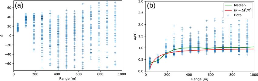
Appendix A
The lidar photon-counting data range was corrected for trig-
ger delay relatively to the analogue data range using the
following procedure. Assuming a linear relation between
photon-counting and analogue data (i.e. no saturation) and
after correcting the latter for voltage offset and dividing it by
the proportionality constant between the two, it is possible to
write the following equations:
f (R)
A= , (A1)
R2
f (R − 1)
PC = , (A2)
(R − 1)2
Figure 19. Aerosol backscattering coefficient (11 February 2021, where A is the corrected analogue signal, PC is the photon-
19:45–20:44 UTC); comparison between the overlap-corrected counting signal, f (R) is a function encompassing all the li-
(solid black line) and uncorrected (dashed red line) profile. dar equation terms apart from the inverse square law, and 1
is the spatial delay between analogue and photon-counting
sampling ranges.
For low R a limited dependence of the function f on R
variations with respect to the inverse square law can be as-
focus image and identified the correct z position. As a result,
sumed. This is true especially for the first bins where limited
the signal intensity increased in the whole channel 1 profile
or no overlap is present and most of the signal comes from
with respect to the previous configuration. The effectiveness
laser secondary reflections and multiple scattering:
of the procedure was verified comparing the results of a tele-
cover test before and after the alignment. The new configu- f (R) ∼ f (R − 1). (A3)
ration resulted in a lower full overlap height (from 1500 m to
less than 1000 m). Under this assumption, the ratio of the analogue and photo-
Once an optimized position has been selected and veri- counting signals is
fied, a laser beam mapping with the purpose of estimating the
overlap function was performed. The retrieved function was A (R − 1)2
(R) = , (A4)
compared to the ones modelled using as input the parame- PC R2
ters obtained from the procedure showing good agreement.
Correcting the lidar profiles of channel 1 with this function from which it is possible to derive the difference 1 as a func-
allows extending the useful range down to 200 m. tion of R:
The developed mapping procedure will be applied to the r !
A
remaining channels in order to characterize each transmitter– 1 (R) = −R −1 . (A5)
PC
receiver combination. Based on the retrieved information
it will be possible to define a set of configurations aimed
Figure A1a depicts the retrieved spatial delay computed with
to satisfy the different scientific objectives (e.g. PBL, up-
Eq. (A5) using laser mapping data from Sect. 4.3. The as-
per troposphere–lower stratosphere). A simplified mapping
sumptions hold for the first two bins from which a delay of
procedure can be used to complement the standard EAR-
∼ 25 m can be derived using an average value. For higher
LINET quality assurance tests. For example, a protocol cou-
ranges, the overlap function dependency from R begins to
pling telecover test and mapping session are currently im-
be relevant, preventing the computation of the delay (i.e. the
plemented in the RMR system. Monthly mappings are per-
assumption in Eq. (A3) is not valid anymore). This depen-
formed to monitor and optimize the alignment and to es-
dency is not definite and partially randomized due to the vari-
timate the overlap function, whereas periodically required
able emitting geometry and resulting overlap function of the
telecover tests (e.g. 1–2 times per year) check and attest the
mapping lidar profiles. Once a delay is retrieved the A/PC
obtained alignment and identify the minimum height with
ratio can be plotted and compared with the range function
full overlap.
(R − 1)2 /R 2 (Fig. A1b). As shown in Fig. A1b, the com-
Besides the applications presented in this study, a simi-
puted range function represents the normalized ratio well.
lar approach could be adapted also to lidar systems with dif-
ferent hardware capabilities to provide essential information
about their transmitter–receiver geometry that is needed for
a complete characterization of the received signal.
https://doi.org/10.5194/amt-15-1217-2022 Atmos. Meas. Tech., 15, 1217–1231, 20221230 M. Di Paolantonio et al.: A procedure for lidar geometry characterization
Figure A1. Spatial delay (a) and ratio A/PC (b) as a function of range.
Code and data availability. Code and data are available upon re- Mazzola, M., Lanconelli, C., Vitale, V., Congeduti, F., Dionisi,
quest by contacting the authors. D., Cardillo, F., Cacciani, M., Casasanta, G., and Nakajima, T.:
Monitoring of Eyjafjallajökull volcanic aerosol by the new Euro-
pean Skynet Radiometers (ESR) network, Atmos. Environ., 48,
Author contributions. MDP, GLL, and DD conceived the concept 33–45, https://doi.org/10.1016/j.atmosenv.2011.09.070, 2012.
of this study. MDP, GLL, and DD performed the lidar measure- Chourdakis, G., Papayannis, A., and Porteneuve, J.: Analy-
ments. MDP developed the presented methods, processed the data, sis of the receiver response for a noncoaxial lidar sys-
and carried out the analysis. MDP, GLL, and DD contributed to the tem with fiber-optic output, Appl. Opt., 41, 2715–2723,
interpretation, the validation, and the visualization of the results. https://doi.org/10.1364/AO.41.002715, 2002.
MDP wrote the original draft with input from all other co-authors. Comeron, A., Sicard, M., Kumar, D., and Rocadenbosch, F.: Use of
All co-authors provided the review and the editing of the paper. a field lens for improving the overlap function of a lidar system
employing an optical fiber in the receiver assembly, Appl. Opt.,
50, 5538–5544, https://doi.org/10.1364/AO.50.005538, 2011.
Competing interests. The contact author has declared that neither Congeduti, F., Marenco, F., Baldetti, P., and Vincenti, E.: The
they nor their co-author has any competing interests. multiple-mirror lidar “9-eyes,” J. Opt. Pure Appl. Opt., 1, 185–
191, https://doi.org/10.1088/1464-4258/1/2/012, 1999.
D’Amico, G., Amodeo, A., Baars, H., Binietoglou, I., Freuden-
thaler, V., Mattis, I., Wandinger, U., and Pappalardo, G.:
Disclaimer. Publisher’s note: Copernicus Publications remains
EARLINET Single Calculus Chain – overview on method-
neutral with regard to jurisdictional claims in published maps and
ology and strategy, Atmos. Meas. Tech., 8, 4891–4916,
institutional affiliations.
https://doi.org/10.5194/amt-8-4891-2015, 2015.
D’Aulerio, P., Fierli, F., Congeduti, F., and Redaelli, G.: Analy-
sis of water vapor LIDAR measurements during the MAP cam-
Acknowledgements. We acknowledge Sara Piermarini and Roberto paign: evidence of sub-structures of stratospheric intrusions, At-
Massimo Leonardi for the development of the first versions of the mos. Chem. Phys., 5, 1301–1310, https://doi.org/10.5194/acp-5-
motor control software. We also acknowledge Raffaello Foldes for 1301-2005, 2005.
his contribution in the early development of the mapping procedure. Dho, S. W., Park, Y. J., and Kong, H. J.: Experimental deter-
We thank Francesco Cardillo for the help in performing lidar mea- mination of a geometric form factor in a lidar equation for
surements. an inhomogeneous atmosphere, Appl. Opt., 36, 6009–6010,
https://doi.org/10.1364/AO.36.006009, 1997.
Dionisi, D., Congeduti, F., Liberti, G. L., and Cardillo, F.: Cal-
Review statement. This paper was edited by Simone Lolli and re- ibration of a Multichannel Water Vapor Raman Lidar through
viewed by two anonymous referees. Noncollocated Operational Soundings: Optimization and Char-
acterization of Accuracy and Variability, J. Atmos. Ocean. Tech-
nol., 27, 108–121, https://doi.org/10.1175/2009JTECHA1327.1,
2010.
References Dionisi, D., Keckhut, P., Hoareau, C., Montoux, N., and Congeduti,
F.: Cirrus crystal fall velocity estimates using the Match method
Cairo, F., Congeduti, F., Poli, M., Centurioni, S., and Di Don- with ground-based lidars: first investigation through a case study,
francesco, G.: A survey of the signal-induced noise in photomul- Atmos. Meas. Tech., 6, 457–470, https://doi.org/10.5194/amt-6-
tiplier detection of wide dynamics luminous signals, Rev. Sci. In- 457-2013, 2013a.
strum., 67, 3274–3280, https://doi.org/10.1063/1.1147408, 1996. Dionisi, D., Keckhut, P., Liberti, G. L., Cardillo, F., and Con-
Campanelli, M., Estelles, V., Smyth, T., Tomasi, C., Martìnez- geduti, F.: Midlatitude cirrus classification at Rome Tor Ver-
Lozano, M. P., Claxton, B., Muller, P., Pappalardo, G., gata through a multichannel Raman–Mie–Rayleigh lidar, Atmos.
Pietruczuk, A., Shanklin, J., Colwell, S., Wrench, C., Lupi, A.,
Atmos. Meas. Tech., 15, 1217–1231, 2022 https://doi.org/10.5194/amt-15-1217-2022M. Di Paolantonio et al.: A procedure for lidar geometry characterization 1231 Chem. Phys., 13, 11853–11868, https://doi.org/10.5194/acp-13- Sherlock, V., Garnier, A., Hauchecorne, A., and Keckhut, P.: Imple- 11853-2013, 2013b. mentation and validation of a Raman lidar measurement of mid- Dionisi, D., Barnaba, F., Diémoz, H., Di Liberto, L., and Gobbi, G. dle and upper tropospheric water vapor, Appl. Opt., 38, 5838– P.: A multiwavelength numerical model in support of quantitative 5850, https://doi.org/10.1364/AO.38.005838, 1999. retrievals of aerosol properties from automated lidar ceilome- Sicard, M., Rodríguez-Gómez, A., Comerón, A., and Muñoz- ters and test applications for AOT and PM10 estimation, At- Porcar, C.: Calculation of the Overlap Function and Associated mos. Meas. Tech., 11, 6013–6042, https://doi.org/10.5194/amt- Error of an Elastic Lidar or a Ceilometer: Cross-Comparison 11-6013-2018, 2018. with a Cooperative Overlap-Corrected System, Sensors, 20, Donovan, D. P., Whiteway, J. A., and Carswell, A. I.: Correction for 6312, https://doi.org/10.3390/s20216312, 2020. nonlinear photon-counting effects in lidar systems, Appl. Opt., Stelmaszczyk, K., Dell’Aglio, M., Chudzyński, S., Stacewicz, T., 32, 6742–6753, https://doi.org/10.1364/AO.32.006742, 1993. and Wöste, L.: Analytical function for lidar geometrical com- Freudenthaler, V.: Effects of Spatially Inhomogeneous Photomul- pression form-factor calculations, Appl. Opt., 44, 1323–1331, tiplier Sensitivity on LIDAR Signals and Remedies, Eur. Space https://doi.org/10.1364/AO.44.001323, 2005. Agency Spec. Publ. ESA SP, 561, 37, 2004. Tomine, K., Hirayama, C., Michimoto, K., and Takeuchi, N.: Exper- Freudenthaler, V., Linné, H., Chaikovski, A., Rabus, D., and Groß, imental determination of the crossover function in the laser radar S.: EARLINET lidar quality assurance tools, Atmos. Meas. Tech. equation for days with a light mist, Appl. Opt., 28, 2194–2195, Discuss. [preprint], https://doi.org/10.5194/amt-2017-395, in re- https://doi.org/10.1364/AO.28.002194, 1989. view, 2018. Wandinger, U. and Ansmann, A.: Experimental determination of the Guerrero-Rascado, J. L., Costa, M. J., Bortoli, D., Silva, A. M., Lya- lidar overlap profile with Raman lidar, Appl. Opt., 41, 511–514, mani, H., and Alados-Arboledas, L.: Infrared lidar overlap func- https://doi.org/10.1364/AO.41.000511, 2002. tion: an experimental determination, Opt. Express, 18, 20350– Wandinger, U., Freudenthaler, V., Baars, H., Amodeo, A., En- 20369, https://doi.org/10.1364/OE.18.020350, 2010. gelmann, R., Mattis, I., Groß, S., Pappalardo, G., Giunta, A., Halldórsson, T. and Langerholc, J.: Geometrical form fac- D’Amico, G., Chaikovsky, A., Osipenko, F., Slesar, A., Nico- tors for the lidar function, Appl. Opt., 17, 240–244, lae, D., Belegante, L., Talianu, C., Serikov, I., Linné, H., Jansen, https://doi.org/10.1364/AO.17.000240, 1978. F., Apituley, A., Wilson, K. M., de Graaf, M., Trickl, T., Jenness, J. R., Lysak, D. B., and Philbrick, C. R.: Design of a li- Giehl, H., Adam, M., Comerón, A., Muñoz-Porcar, C., Roca- dar receiver with fiber-optic output, Appl. Opt., 36, 4278–4284, denbosch, F., Sicard, M., Tomás, S., Lange, D., Kumar, D., https://doi.org/10.1364/AO.36.004278, 1997. Pujadas, M., Molero, F., Fernández, A. J., Alados-Arboledas, Kokkalis, P.: Using paraxial approximation to describe the op- L., Bravo-Aranda, J. A., Navas-Guzmán, F., Guerrero-Rascado, tical setup of a typical EARLINET lidar system, Atmos. J. L., Granados-Muñoz, M. J., Preißler, J., Wagner, F., Gausa, Meas. Tech., 10, 3103–3115, https://doi.org/10.5194/amt-10- M., Grigorov, I., Stoyanov, D., Iarlori, M., Rizi, V., Spinelli, 3103-2017, 2017. N., Boselli, A., Wang, X., Lo Feudo, T., Perrone, M. R., De McGill, M. J., Yorks, J. E., Scott, V. S., Kupchock, A. W., and Tomasi, F., and Burlizzi, P.: EARLINET instrument intercompar- Selmer, P. A.: The Cloud-Aerosol Transport System (CATS): a ison campaigns: overview on strategy and results, Atmos. Meas. technology demonstration on the International Space Station, in: Tech., 9, 1001–1023, https://doi.org/10.5194/amt-9-1001-2016, Lidar Remote Sensing for Environmental Monitoring XV, Proc. 2016. Spie., 96120A, https://doi.org/10.1117/12.2190841, 2015. Weitkamp, C. (Ed.): Lidar: range-resolved optical remote sens- Measures, R. M.: Laser remote sensing: Fundamentals and appli- ing of the atmosphere, Springer, New York, 455 pp., 1st Edn., cations, John Wiley & Sons, Inc., Hoboken, 1st Edn., 510 pp., https://doi.org/10.1007/b106786, 2005. ISBN: 978-0-471-08193-7, 1984. Wiegner, M., Madonna, F., Binietoglou, I., Forkel, R., Gasteiger, J., Pappalardo, G., Amodeo, A., Apituley, A., Comeron, A., Freuden- Geiß, A., Pappalardo, G., Schäfer, K., and Thomas, W.: What thaler, V., Linné, H., Ansmann, A., Bösenberg, J., D’Amico, is the benefit of ceilometers for aerosol remote sensing? An G., Mattis, I., Mona, L., Wandinger, U., Amiridis, V., Alados- answer from EARLINET, Atmos. Meas. Tech., 7, 1979–1997, Arboledas, L., Nicolae, D., and Wiegner, M.: EARLINET: to- https://doi.org/10.5194/amt-7-1979-2014, 2014. wards an advanced sustainable European aerosol lidar network, Winker, D. M., Pelon, J. R., and McCormick, M. P.: CALIPSO Atmos. Meas. Tech., 7, 2389–2409, https://doi.org/10.5194/amt- mission: spaceborne lidar for observation of aerosols and 7-2389-2014, 2014. clouds, in: Lidar Remote Sensing for Industry and Environ- Sasano, Y., Shimizu, H., Takeuchi, N., and Okuda, M.: Ge- ment Monitoring III, P. Soc. Photo.-Opt. Ins., 4893, 1–11, ometrical form factor in the laser radar equation: an https://doi.org/10.1117/12.466539, 2003. experimental determination, Appl. Opt., 18, 3908–3910, https://doi.org/10.1364/AO.18.003908, 1979. https://doi.org/10.5194/amt-15-1217-2022 Atmos. Meas. Tech., 15, 1217–1231, 2022
You can also read