A robust nuclear strategy for France
←
→
Page content transcription
If your browser does not render page correctly, please read the page content below
A robust nuclear strategy for France
                                        PERRIER, Quentin
                                     quentin.perrier@ehess.fr

                                        November 19, 2016

                                                Abstract
         After the first oil shock, France fully engaged in the world’s largest nuclear program,
     ordering 36 reactors within two years. These reactors are now reaching the end of their
     lifetime, so a new policy must be defined: Should they be retrofitted or decommissioned?
     What are the prospects for nuclear afterwards? The best economic decision crucially depends
     on the future costs of nuclear, demand levels and CO2 price, which are all subject to significant
     uncertainty.
         In face of these uncertainties, we apply the framework of Robust Decision Making to de-
     termine which plants should be retrofitted. We build and use an optimization model of invest-
     ment and dispatch, calibrated for France, and study 27 retrofit strategies for all combinations
     of uncertain parameters.
         Based on nearly 3,000 runs, our analysis reveals one robust strategy, which departs from
     optimal non-robust strategies and from the French official scenarios. This strategy implies
     to shut down more than 80% of the oldest nuclear reactors up to 2020, i.e. between 11 and
     14 reactors, and then extend the lifetime of all remaining reactors. This strategy provides a
     hedge against unexpected high retrofit cost, decreasing demand or low CO2 price.
         In the longer term, we show that the optimal share of nuclear in the power mix decreases.
     If the cost of new reactors (EPR or else) remains higher than 80 e/MWh, this optimal share
     drops below 40% in 2050. A combination of variable renewables, hydropower and gas becomes
     more competitive, even if the price of CO2 reaches 200 euros/tCO2 .

1    Introduction
After the first oil shock, France has engaged in an unprecedented nuclear program, which would
make it up to now the country with the highest share of nuclear in its power mix. The first Contract
Program was launched in 1969. A batch of six reactors of 900 MWe were ordered (the CP0 batch)
and their construction started in 1971. But the first oil shock triggered a more ambitious nuclear
program. In early 1974, 18 identical reactors of 900 MWe were ordered (CP1 batch). They were
followed in late 1975 by 18 new reactors : 10 reactors of 900 MWe (CP2 batch) and 8 of 1300 MWe
(CP4 batch). 12 additional reactors of 1300 MWe were ordered in 1980 (P’4 batch). Finally, in
1984, 4 reactors of 1450 to 1500 MWe (N4 batch) concluded this nuclear policy (Boccard, 2014).
These massive orders have been shaping power production in France ever since. In 2015, these
nuclear plants produced 78% of its electricity. With a 12% of hydropower production, it leaves
only around 10% for all other sources of power (RTE, 2014).
    But these power plants are now reaching the end of their lifetime. The reactors were initially
designed to last for 32 years at nominal power and 40 years at 80% of their nominal power(Charpin
et al., 2000, p.31). In practice, the 40 years threshold is used by the national authority on nuclear
safety, the ASN. These reactors are now reaching this 40 years limit. The first ones will be the two
reactors in Fessenheim, which will reach 40 years in 2017.
    The lifetime of these nuclear plants can be extended if refurbishment works are undertaken.
Thus, a new nuclear policy must be decided: should these plants be retrofitted? And more gen-
erally, what is the future of nuclear in France? These questions are now at the heart of a public
debate. The diversity of opinions on this matter was highlighted by the French National Debate
on Energy Transition in 2012. The views on the future of nuclear in France ranged from a fully

                                                    1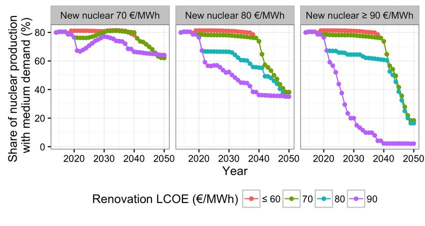
maintained nuclear share, to partial refurbishment strategies, to a full and early phase-out (Arditi
et al., 2013).
    These disagreements stem in large part from different estimations of nuclear costs and risks.
The cost of retrofitted and new nuclear, in particular, is subject to some uncertainty. Various
elements stretch the range of plausible future costs.
    On the one hand, the recent literature and events about nuclear costs presents arguments
supporting the ideas of increasing costs in the future. The main arguments contending that a
decrease in nuclear costs is unlikely are:

      • negative learning-by-doing: The French nuclear industry has been facing "negative learning-
        by-doing" in the past, although it benefited from a very favourable institutional environment
        (Grubler, 2010).
      • increased safety pressure: Increased safety pressure can increase costs. In particular, the
        Fukushima accident has led the French nuclear regulator, the ASN, to impose new safety
        measures.
      • recent and unexpected cost surge: the EPR technology in Flamanville (France) has been
        delayed several times, and its costs tripled. The EPR in Olkiluoto (Finland) is also facing
        several difficulties. This is raising doubts about the ability of EDF to build power plants of
        the EPR technology. As to retrofitting the historic power plant, the first retrofit has led to
        an incident which may cause delays and significant cost increases1 ;
      • high contract price for nuclear: in the UK, EDF signed a contract at 92.5 £/MWh
        (118 e/MWh at 2015 exchange rate) and indexed on inflation, which means the nominal
        price will be higher when the plant starts to produce. The exact costs of the French EPR are
        difficult to assess as they are not publicly displayed. This market price is thus an important
        clue as to the cost of this technology.
      • unexpected stops: The discovery of anomalies has led to reinforced controls. As a conse-
        quence, in October 2016, 12 reactors our of 58 were stopped to check the resistance of their
        steam turbines (Monicault, 2016). This lead to concerns about the security of supply and
        the future load factor of these plants, which is a key parameter of their value (Internationale
        Energy Agency and Nuclear Energy Agency, 2015).
      • risks and insurance costs: The Fukushima accident has prompted a renewed interest
        on the question of insurance costs from Cour des Comptes (2012). This insurance should
        match the criticality of nuclear, i.e. the probability of an accident multiplied by severity of
        the consequences (although the French nuclear operator EDF has benefited from a limited
        liability). However, both probability and damage costs are difficult to estimate. To give
        an idea of these uncertainties, Boccard (2014) estimates this insurance cost at 9.6 e/MWh,
        while Lévèque (2015) provides an expected cost of nuclear disaster below 1 e/MWh.

    On the other hand, constructing several reactors of the same type can lead to learning-by-doing
in the construction process. Standardization reduces lead times and thus reduces the cost of this
technology. The size of reactors is also positively correlated with cost (Rangel and Leveque, 2015).
A standardized approach with smaller reactors could thus stop the negative learning-by-doings and
even decrease the future costs of nuclear.
    These elements should encourage carefulness when assessing the future costs of nuclear. They
entail that a wide range of costs can be considered as plausibl e, in the sense that they cannot be
immediately dismissed since some elements support them. In addition, these uncertainties are in
multiplied by other uncertainties on demand, CO2 price and renewable costs.
    Our aim is to analyse optimal nuclear policies, but also to determine policies that are robust
to these various uncertainties. Part II examines in more details the various sources of uncertainty.
Part III presents the optimization model. Part IV shows the results of optimization. Part V
adds robustness to the analysis. Part VI compares our results to the national debate on energy
transition. Part VII concludes.
  1   on March 31, 2016, a steam generator of 465 tonnes and 22m high fell during its replacement operation

                                                        2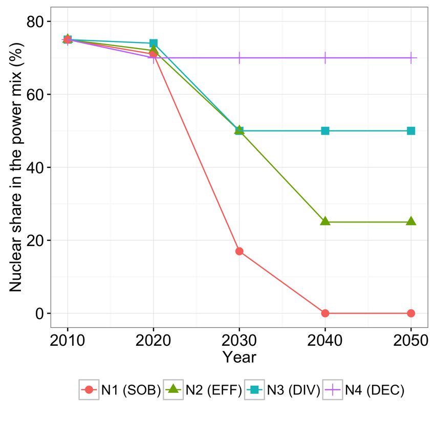
2     Method: Dealing with uncertainties for nuclear prospects
Knight (1921) made an important distinction between risk and uncertainty. There is a risk when
change can happen, for example in the value of a parameter, but the probability of any particular
occurrence is measurable and known. When these probabilities are not known, there is uncertainty.
    In the case of nuclear, the future costs are not known, and their probability of occurrence
cannot be measured. The same holds true for demand levels, CO2 prices and renewable costs.
We are dealing with a situation of uncertainty in the sense of Knight. In such situations, the
traditional approach of practitioners is to employ sensitivity analysis (Saltelli et al., 2000). An
optimum strategy is determined for some estimated value of each parameter, and then tested
against other parameter values. If the optimum strategy is insensitive to the variations of the
uncertain parameters, then the strategy can be considered a robust optimum.
    However, when no strategy is insensitive to parameter changes, it is not possible to conclude
to a single optimum strategy or policy. On the contrary, several optimal strategies coexist, each
being contingent to the model specifications. In other words, each optimum is linked to some
specific future(s). For example, in our case, it could be optimal to retrofit for some plausible costs
of retrofitting, but not optimal for other plausible costs.
    Having a multiplicity of optimal scenarios is not a practical tool for choosing one strategy. A
decision-maker would be interested by a strategy that performs well over a large panel of futures,
i.e. a robust strategy, even if it means departing from an optimal non-robust strategy. In our
case of uncertainty, it means to determine a robust scenario without assuming a distribution of
probabilities. This concept of robustness is not new, but it has received a renewed interest with
the increase of computational power, and with the issue of climate change Hallegatte (2009).
    In this paper, we use the Robust Decision Making (thereafter RDM) framework developed by
Lempert et al. (2006) to study the future of nuclear in France under uncertainty. This methodol-
ogy has already been applied to study the robustness of the power system to unexpected shocks
Nahmmacher et al. (2016).

2.1     Presentation of the RDM framework
The RDM framework uses the notion of regret introduced by Savage (1954). The regret of a
strategy is defined as the difference between the performance of that strategy in a future state of
the world, compared to the performance of what would be the best strategy in that same future
state of the world. To formalize it, the regret of a strategy s 2 S in a future state of the world
f 2 F , is defined as:

                  regret(s, f ) = M ax{P erf ormance(s0 , f )}   P erf ormance(s, f )
    where s goes through all possible strategies. Performance is measured though an indicator.
            0

In our case, it will be to cost minimization. The regret is then equivalent to the cost of error of
a strategy, i.e. the cost of the chosen strategy compared to the cost of what would have been
the best strategy. The regret indicator allows to measure when a strategy performs better than
another. In addition, regret has the property of preserving the ranking which would result from
any probability distribution. We can thus use this indicator without inferring any probability of
distribution ex ante, and apply different probability distribution ex post.
    The RDM method proceeds in several steps:
    1. Define the set of plausible future states of the world F . By plausible, we mean any parameter
       value and model specification that cannot be excluded ex ante. The idea is to have a large
       set, as a set too narrow could lead to define strategies to could end up being vulnerable to
       certain futures that were dismissed.
    2. Define a set of strategies S. In our case, it means to define different policies as to the
       refurbishment of nuclear plants. For example, a strategy could be to refurbish the 58 reactors;
       another policy, to refurbish every other reactor, and so on.
    3. Identify a initial candidate strategy scandidate 2 S. This strategy can be chosen as the most
       robust one when considering all futures F , or according to other criteria. This choice is not
       structuring for the conclusions, it is only a step in the process.

                                                   3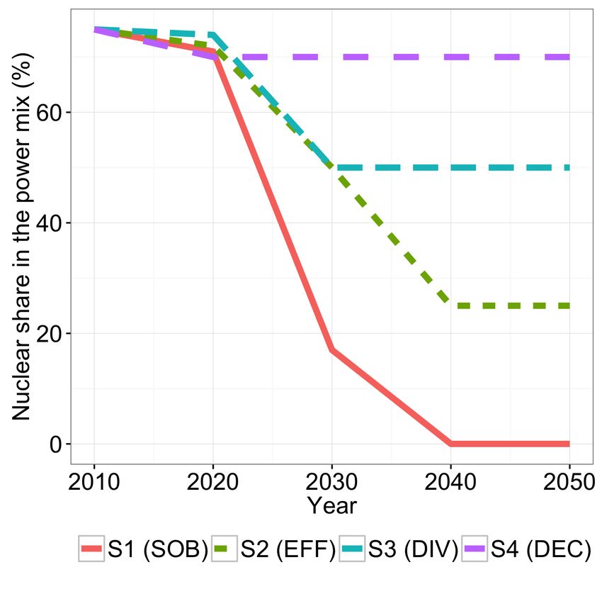
4. Identify the vulnerabilities of this strategy. This step is based on statistical methods in order
     to determine one or several subsets of the futures states of the world Fvuln i
                                                                                      (scandidate ) 2 F ,
     in which the candidate strategy scandidate does not perform well. A threshold must be
     defined
          P toi decide what is acceptable. By elimination, we can also deduct the subset F =
                                                                                                     0

     F       Fvuln (scandidate ) in which the candidate strategy is robust.

  5. Identify alternative strategies. For each subset Fvuln
                                                        i
                                                             (scandidate ) and for F 0 , we rank all the
     strategies in terms of regret, and identify the best strategy in terms of regret.
  6. Characterize the trade-offs between the various robust strategies. Each strategy has a differ-
     ent regret for each subset Fi and F 0 . Some strategies will have low regret in one subset and
     a high regret in the other; other strategies will have medium regrets. It is then possible to
     draw a low-regret frontier and highlight the few alternative strategies on that frontier.

2.2    Description of the candidate strategies
In order to identify a robust strategy, we define several trajectories of nuclear refurbishment. The
58 reactors offer 258 =2.9*1017 possibilities. As we aim to test each candidate strategy against
multiple values of uncertain parameters, this problem could turn too computable-intensive. Thus,
we simplify this problem, with the aim to keep the diversity of possible trajectories. We split the
reactors into three groups, according to the end of their initial 40 years lifetime. The first group
includes of all reactors which will reach 40 years before 2021, which includes 14 reactors. The
second group includes all reactors reaching 40 years between 2021 and 2025, or 23 reactors. The
last group includes the 21 remaining reactors.
    For each group, we consider three possibilities: i) all reactors are refurbished; ii) every other
reactor is refurbished and iii) no reactor is refurbished. We end up with 33 =27 different strategies.
This split in three periods is meant to take into account the time-dimension of a retrofit strategy.
It enables to explore whether an early retrofit (or phase-out) should be preferred over a late retrofit
(or phase-out). In addition, it provides a good covering of the possible strategies, as shown in fig. 1.
More information on these strategies can be found in table 10.

       Figure 1: Nuclear capacity of existing plants, including retrofit, in the 27 strategies

2.3    Related literature on power transition and nuclear
Many studies analyze a low-carbon transition in the power sector, at a national level (Fraunhofer
Institute, 2015) or a European level (Jägemann et al., 2013; European Commission, 2012). Focusing
more specifically on nuclear, Bauer et al. (2012) study the cost of early nuclear retirement at the
world level, and show that the cost of nuclear phase-out is an order of magnitude lower that the

                                                   4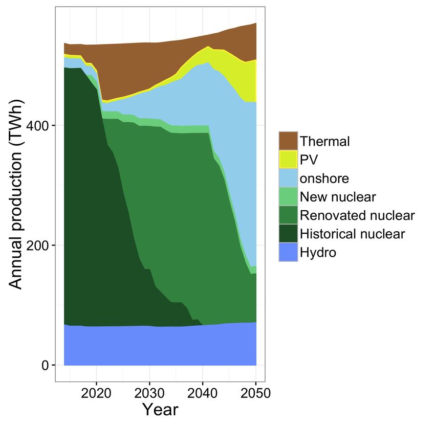
cost of a climate policy. But this result might not hold for France as the share of nuclear is much
higher than world average.
    For France, the French Energy Agency, ADEME, produced a study of renewable penetration in
2050 (ADEME, 2015). However, they do not study the path between today and 2050: the power
mix was built ex nihilo (greenfield optimization) in 2050 as an optimization with 2050 projected
costs. Petitet et al. (2016) study wind penetration in France, but without modeling the potential
of hydro optimization to smooth wind penetration, and consider only cases in which nuclear is
cheaper than wind - a debatable assumption, as we will show.
    Our paper contributes to the literature in several points. The first and main one is to deal
explicitly with the high uncertainty on nuclear costs, rather than using specific -and controversial-
values. In addition, we provide a model to study nuclear and renewables with around 12% hydro
and optimized pumped storage, while the literature has focus mainly on thermal power systems, and
seldom on power system with a high share of hydro (Hirth, 2016). Finally, we provide trajectories
of nuclear for France, which is often difficult to represent properly in models covering a larger
region.
    We now apply the RDM framework to identify a robust nuclear policy. First, we must first
estimate the range of plausible values for the various uncertain parameters. This is the topic of
section 3. Then, we present our optimization model in section 4. Next, we run our optimization
model for our 27 strategies and all plausible values of the uncertain parameters. We present the
results in section 5. Section 6 compares our results with the French official scenarios which stemmed
from the national debate on energy transition. Section 7 concludes.

3     Defining plausible values
3.1     Cost of retrofitted PWR plants
The cost of the French historic technology has been the focus of a few papers. The first official
report on the historic French nuclear program was made by Charpin et al. (2000). It was later
analyzed by Grubler (2010), who evidenced cost escalation in time, which he coined as "negative
learning-by-doing". Based on the 2012 ’Cour des Comptes’2 report, Rangel and Leveque (2015)
also examined this cost escalation, and evidenced a learning curve within technologies of the same
type and size. Finally, using a new audit launched after the Fukushima accident, Boccard (2014)
reveals larger than expected operation costs for French reactors: 188 e/kW/year, or more than
25 e/MWh with the historical load factor. This value is a key determinant of total retrofit cost,
since fixed capital costs are already amortized to a large extent. And this estimate is much higher
than the value suggested by Internationale Energy Agency and Nuclear Energy Agency (2015) at
13,3 e/MWh.
    These old reactors now reach the end of their initially planned lifetime of forty years3 . These
lifetimes can be extended, but only if some upgrade work is performed. A new report published
by the French court of audit provides the cost estimates of refurbishment by EDF, the French
operator of nuclear plants. These estimates range around e100 billion up to 2030: e74.73 billion
of additional investment and e25.16 billion of additional O&M costs (Cour des Comptes, 2016).
Between 2014 and 2030, 53.2 GW will reach the limit of 40 years, yielding an average additional
cost of 1,880 e/kW. To translate these values into LCOE, one needs to make assumptions about
capital cost, load factor and lifetime.
    Financial costs are highly dependent on the rate at which capital is borrowed. In France,
Quinet (2013) recommends to use a rate of 4.5% for public investments. The IEA uses a rate of
5%, which we use for our best case scenario, to account for financial costs. We use a rate of 10%
for our worst case scenario, following Boccard (2014).
    For the load factor, we use the latest estimates by Cour des Comptes (2016, p. 116), which
shows that the availability of French nuclear plants has oscillated between 83.5% and 78% since
2005. We link these values to respectively a best case and a worst case.
   2 The Court of Auditors (in French Cour des Comptes) is a quasi-judicial body of the French government charged

with conducting financial and legislative audits of most public institutions
   3 French reactors were initially designed for a lifetime of forty years, with a count start at their first nuclear

reaction. In the US, lifetime is counted from the first layer of concrete.

                                                         5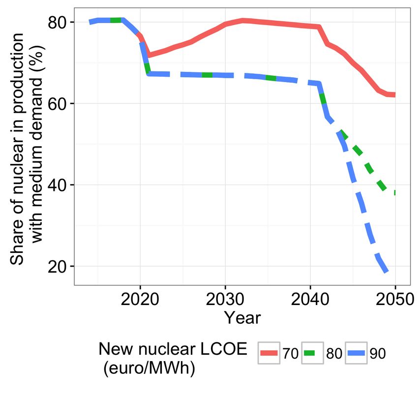
Table 1: Cost of a retrofitted French power plant (e/MWh)

                                              20 years extension     10 years extension
                                              Low          High      Low          High
                  Additional investment       13.0           20.4    21.0            28.2
                  Additional O&M costs         4.4            6.9     7.1             9.5
                  Historic O&M                13.3           27.5    13.3            27.5
                  Fuel costs                   6.6            6.6     6.6             6.6
                  Back-end                     1.8            1.8     1.8             1.8
                  Total                       39.4           63.1    49.7            73.6
The best case is an extension of twenty years without additional cost; the worst case is a decom-
missioning after ten years. The "low" costs are obtained for capacity factor of 83.5% and a capital
cost of 5%, against 78% and 10% respectively for the "high" costs.
Source: Author’s calculations based on Boccard (2014) and Cour des Comptes (2016)

    As to lifetime, we suppose that the investment of extending the lifetime will enable the plant
to run for 20 more years. There is significant uncertainty around this last assumption. In France,
nuclear plants are given license by slice of ten years. The French Authority of Nuclear Safety
seems willing to provide licenses for a ten years extension; but there is no certainty that it will
give its approval in ten years for another extension. It may decide to close some plants, or ask
for additional investment at that time. However, the magnitude of the investment indicates that
EDF is confident it will be able to run for 20 years without too much additional cost. Thus, this is
the central hypothesis we retain in the following of this paper (but we also look at a less favorable
scenario in which the first extension is followed by a decommissioning in our cost estimates).
    From this literature, we compute new estimates of the LCOE of retrofitted power plants in
France. Nuclear plants can be extended by ten or twenty years. For these two possibilities, we
compute a low and a high estimate. In the low estimate, we suppose a capacity factor of 83.5%
and a financial cost of 5%. For operating costs (O&M, fuel and back-end), we use the values from
Internationale Energy Agency and Nuclear Energy Agency (2015). For the high estimate, capacity
factor and financial costs are 78% and 10% respectively, and operating costs are derived from
Boccard (2014) 4 . For the rest, we use the latest figures from Cour des Comptes (2016). We get a
LCOE in the range of 39-63e/MWh in our best case for an extension of twenty years, and 50-74
e/MWh for an extension of ten years. These figures are detailed in table 1. But it is important to
note that no plant has undergone a full retrofit yet. Thus, these estimates are still uncertain, and
could increase in case of unexpected difficulties. In addition, these costs do not include the cost of
insurance. This issue is investigated in section 3.3, as it also applies to new nuclear, which is the
topic of the next session.

3.2    Cost of new nuclear plants
In parallel to retrofitting its existing reactors, EDF has developed a new technology: the European
Pressurized Reactor (EPR). However, this model has also faced serious setbacks. The yet unfinished
reactor developed in France saw its cost rising from a initially planned e3 billion to e10.5 billion.
In Finland, the construction work for an EPR reactor started in 2005 with a connection initially
scheduled in 2009, but has so far been delayed until 2018. In the UK, the EPR has been negotiated
at 92.5 £/MWh – approximately 127 e/MWh at the exchange rate of 2015 given by Eurostat.
    As to the future of the EPR cost, a tentative cost is estimated by Boccard (2014) between
76 and 117 e/MWh, for a total cost of e8.5 billion (before its upwards adjustment to e10.5
billion) when taking including back-end and insurance costs (he estimates insurance costs at around
9.6 e/MWh). The high end is in line with the contract price of the Hinkley point reactor. A
wide spread is found in the literature, from 76 e/MWh to 120 e/MWh, as shown in fig. 2. In
addition, the cost of nuclear has been shown to depend on safety pressure. For example, Cooper
   4 We use estimates by Boccard in e/kW/year, but our projected capacity factor is slightly higher than his

historical (78% and 83% vs 76%), which gives use lower costs in e/MWh compared to his numbers.

                                                     6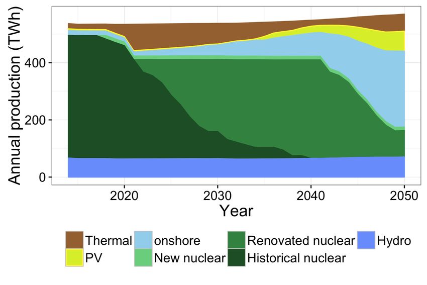
(2011) showed that the Three Mile Island accident had a significant impact on cost escalation.
Consequently, any new incident could increase these current estimates. This creates additional
uncertainty on future nuclear costs. These significant uncertainties about future costs led some to
qualify the nuclear option as a "bet" (Lévèque, 2013).
   This wide range of nuclear cost is critical, as it encompasses the current levels of feed-in tariffs for
wind in France and its LCOE expected in 2050. In France, in 2014, onshore tariff was set between
55 and 82 e/MWh for a lifetime of 20 years (82 e/MWh for the first ten years, and between 28
and 82 e/MWh afterwards, depending on wind conditions) 5 Wind tariffs in neighboring Germany
were set at 59 e/MWh in 2015: 89 e/MWh during 5 years and 49.5 e/MWh afterwards Bundestag
(2014).
   Finally, it is important to note that new nuclear is expected to be costlier than retrofitted
plants. The general idea is that a brown field project (a retrofitted plant) requires less investment
than a greenfield project. This idea is further supported by the cost range estimates in fig. 2.
Thus, we will focus on the cases in which new nuclear is more costly than retrofitted nuclear.

                 Figure 2: LCOE of retrofitted nuclear, new nuclear and wind in France

    There is also an uncertainty on wind cost, due to uncertainty on technological improvements
(e.g. with the potential of larger rotors, see Hirth and Müller (2016)). We will discuss in this paper
the uncertainty of nuclear costs. Implicitly, it is the cost difference with wind and gas which is
meaningful here. Our estimates of gas and wind costs are given in appendix B for the interested
reader.
  5    Note that the wind developer must pay for connexion to and upgrade of the distribution network to access this
FIT.

                                                          7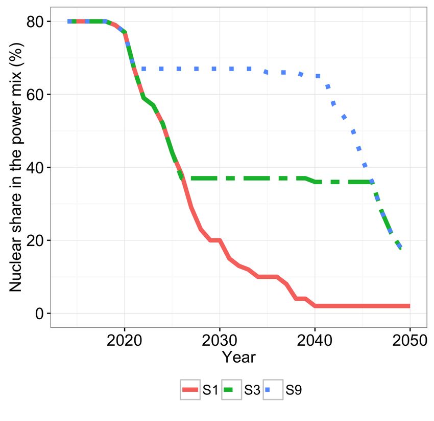
3.3    Cost of a nuclear accident
The Fukushima accident has prompted a renewed interest on the question of insurance costs. The
insurance cost should match the criticality of nuclear, i.e. the probability of an accident multiplied
by severity of the consequences. However, both the probability of an accident and damage costs
are difficult to estimate.
    Damage costs depend on several assumptions about indirect effects, as well as on monetizing
nature and human lives (Gadrey and Lalucq, 2016). Thus, an irreducible uncertainty remains
here. To give an idea of these uncertainties, the IRSN - the French Institute on Nuclear Safety -
estimated the cost of a "controlled" release of radioactive material between 70 and 600 billion euros
(Cour des Comptes, 2012). To give another reference, the Fukushima accident has been estimated
at 160 billion euros by Munich Re (2013).
    To assess the probability of a nuclear accident, two approaches coexist. The first one is the
Probabilistic Risk Assessment (PRA). It consists in a bottom-up approach, which compounds the
probabilities of failures which could lead to a core meltdown. This measure is used by regulators
in the US (Kadak and Matsuo, 2007). Depending on regulators, this PRA varies from 10-4 to 10-6
per year and per reactor (Ha-Duong and Journé, 2014). In France, the probability of an accident
which would release a significant amount of radioactivity in the atmosphere is estimated at 10-6 for
current plants, and 10-8 for the EPR reactor (Cour des Comptes, 2012). However, there is some
uncertainty in knowledge that is not fully captured by this type of analysis, as suggested by the
examples of Three Mile Island, Chernobyl and Fukushima. A wide discrepancy is observed at first
glance between expected number given by the PRA estimate and the number of observed nuclear
accidents worldwide (Ha-Duong and Journé, 2014).
    This discrepancy has motivated another approach, statistical and based on past historical acci-
dents. In particular, the Fukushima accident has prompted a renewal of research based on empirical
estimates. Escobar Rangel and Lévêque (2014) recall that most of the accidents occurred at the
early stage of nuclear power plants. Continuous safety improvements might have improved secu-
rity closer to PRA estimates. They also argue that the Fukushima accident has revealed the risks
associated with extreme natural events and regulatory capture, thus opening the door for further
improvements.
    However, this second approach suffers from two short-comings. The first one is the low number
of occurrences. Only two events are classified in the category of major accident, i.e. a level 7 on
the INES scale - the INES scale, introduced by the International Nuclear Energy Agency, ranges
nuclear events from 1 (anomaly) to 7 (major accident). Most estimates thus study the probability
of a larger pool of event. But the gain in estimation accuracy comes at the cost of a change in
the meaning of the results (Escobar Rangel and Lévêque, 2014). What is measured is not only
the probability of major accident, but also includes the probability of less dramatic events. The
second one comes from the use of past, historical data. This does not enable to account for the
potentially increased risks due to aging power plants, nor for the tensed political situation with
fears of terrorist attacks. This uncertainty can drastically change the cost of insurance. If we
estimate the cost of insurance as the criticality of nuclear or, in other words, its expected cost. If
we assume the cost of a major nuclear accident to be 100 billion euros, as recommended by Cour
des Comptes (2012), then a probability of accident between 10-8 and 10-5 makes the insurance
cost vary from 0.14 e/MWh to 142 e/MWh, as shown in table 2. And that range is in line with
requirement from the regulator for a core meltdown.
    The point behind these figures is that the cost of insurance cannot be dismissed once and for all.
Expectations of security improvements explain an almost negligible value for nuclear insurance,
while a more conservative view can lead to significantly higher estimates.

3.4    Demand, CO2 price and renewable cost
There is some uncertainty on the demand level. This was highlighted during the National Debate
on Energy Transition in France, which led to four contrasted demand scenario: SOB, EFF, DIV
and DEC, in order of increasing demand. Our reference scenario is in line with the DIV scenario,
as it is closest to current projections by the French transmission line operator, RTE. It is roughly
a scenario of flat demand. The most extreme scenarios were SOB, for low demand, and DEC,
for high demand. We use these as our low and high case respectively, to account for all plausible

                                                  8
Table 2: The uncertainty around insurance costs for nuclear for an estimated cost of 100 billion
euros.
Estimated probability of Insurance
an accident cost
(per MW per annum) (euro/MWh)
10 8
0,14
10 7
1,43
10 6
14,27
10 5
142,69
values of demand.
For CO2 , we use the official price used in French public investments as defined in Quinet (2009).
In the central scenario, this price goes up to e100 in 2030 to e200 in 2050. In the short term,
these prices are significantly higher than the price of emission allowances on the EU ETS market
(which has stayed below 10 e/CO2 on the EEX market in the past year) and there is no reason
to think that the EU ETS price might be higher, even with the proposition of back-loading some
allowances in the future (Lecuyer and Quirion, 2016). We also consider a variant with low CO2
price, in which we divide the official price by a factor 2. It thus attains 50 euros in 2030 and 100
euros in 2050. Such a high price reflects the implicit view in all scenarios to phase-out coal and
gas in the long-term, in order to avoid an increase of CO2 emissions. They could also represent
the price floor for CO2 currently discussed in France.
Finally, the cost of renewables is also uncertain. To a large extent, what is relevant in the
competition between nuclear and renewable is their comparative cost. We run the model for many
different costs of both retrofitted and new nuclear. So we get in fact many different comparative
cost. A reader with different assumptions about renewable costs could just correct the thresholds
that we find in terms of nuclear price.
All these uncertainties thus raise the question of the optimal mix. However, the LCOE metric
does not account for "integration costs" (Ueckerdt et al., 2013). Nuclear has the advantage of being
a dispatchable power source, while wind and solar PV are variable. As a consequence, their value
decreases as their penetration rate increases, although the magnitude of this decrease is specific to
the power system (Hirth, 2016) and to the renewable technology characteristics (Hirth and Müller,
2016). This phenomenon of value drop is sometimes called "self-cannibalization effect". Using
an optimization model of the entire power system enables to capture these integration costs. We
present our model in the following section.
4 Model description
The French power model FPM is an optimization model of investment and dispatch. It is a partial
equilibrium model of the wholesale electricity market, which determines optimal investment and
generation. It is designed to study the French power mix, with a particular focus on nuclear
and hydropower. Hourly demand, net exports and CO2 price are exogenous, as well as hydro
capacities. Otherwise, all technologies are endogenous for both investment and dispatch - with a
cap on nuclear retrofitted capacities based on the current fleet of nuclear plants. All the equations
of the model are available at https://github.com/QPerrier/FPM.
4.1 Generation technologies
Twelve generation technologies are modeled: two renewable energies (onshore wind and solar PV),
five thermal technologies (coal plants, combined cycle gas turbine, open cycle gas turbine, fuel
plants), three nuclear technologies (historical nuclear, retrofitted nuclear and new nuclear) and
three hydro systems (run-of-river, conventional dams for lakes and pumped storage). Investment
in each technology is a choice variable of the model, except for hydropower and historical nuclear,
which are exogenous. Generation of each technology is a choice variable, except for run-of-river
production, which is exogenously based on historical data.
9The capacity of run-of-river and conventional dams is supposed to be constant, while the
pumped hydro capacity is supposed to grow by 3.2 GW by 2050, with a discharge time of 20
hours, as in ADEME (2013). Hydro storage and dispatch is optimized by the model, under water
reservoir constraints and pumping losses. Dams receive an amount of water to use optimally at
each period. Pumped hydro can pump water (although there are losses in the process), store it
into a reservoir and release the water through turbines later on.
A particularity of the model is to represent explicitly the cost of extending the lifetime of nuclear
power plants. Nuclear plants normally close after 40 years, but their lifetime can be extended to
60 years, if upgrade costs are paid for. In that sense, they are modeled as a technology with an
investment cost, a lifetime of 20 years, and a constraint that total investment cannot exceed the
capacity decommissioned at any given year. For historical nuclear, we exogenously phase-out the
capacity of each power plant reaching 40 years. The same year it reaches 40 years, this capacity
of a historical nuclear plant is endogenously either extended for 20 years, or phased-out.
Hourly Variable Renewable Energy (VRE) generation is limited by specific generation profiles
based on historical data for the year 2014. Dispatchable power plants produce whenever the price
is above their variable costs, unless they are limited by their ramping constraints. At the end its
lifetime, each capacity is decommissioned. Power generation required for heat generation was on
average 2% of consumption, and never above 5% of consumption in France in 2014 (RTE, 2014),
so we do not model it. The remaining capacity can be optimized for power generation.
4.2 Model resolution
The model invests optimally in new capacities at a yearly step from 2014 to 2050. The dispatch of
generation capacities is computed to meet demand for six representative weeks at an hourly step.
Each typical week represents the average demand of two months of real data, through 168 hours.
For example, demand of Monday for week 1 represents the average demand, on an hourly basis, of
all the Mondays in January and February. This is similar to having 24*7=168 time slices in the
TIMES model6 or in the LIMES-EU model7 . Demand is exogenous and assumed to be perfectly
price inelastic at all times. Net export flows are given exogenously, based on historical data. The
various demand scenarios we study stretch the initial demand profile (domestic consumption plus
exports) homothetically, thus without altering the shape of peak or base demands.
The model covers France as a single region.
At each typical week is associated i) a water inflow for run-of-river and dams, ii) an availability
factor for conventional generation technologies for each representative week, to account for main-
tenance and iii) a production profile for renewable technologies (onshore wind and PV) based on
historical production.
4.3 Objective function
The objective of the model is to minimize total system costs over the period 2014-2050. The cost
of each technology is annualized, both for O&M and capital costs. Capital annuities represent
the payment of the loan. In addition, using annuities allows to avoid a border effect in 2050: the
annual costs are still well represented at the end of the time horizon.
We use a 0% rate of pure time preference, in order to give the them weight to the different
years and generation up to 2050. This assumption is also made in the EMMA model (Potsdam
Institute for Climate Impact Research) used for example by Hirth and Müller (2016). Costs include
investment costs, fixed O&M costs, variable costs and costs due to ramping constraints. To account
for financing cost (e.g. the cost of borrowing), investment costs are annualized with a 5% interest
rate, as in Jägemann et al. (2013). Variable costs are determined by fuel costs, CO2 price, plant
efficiency and total generation.
CO2 price is derived from the official CO2 price used in French public investments, defined in
Quinet (2009). In the central scenario, this price goes up to e100 in 2030 and to e200 in 2050. In
the short term, these prices are significantly higher than the price of emission allowances on the
EU ETS market (which has stayed below 10 e/CO2 on the EEX market in the past year) and
6 http://iea-etsap.org/docs/TIMESDoc-Intro.pdf
7 https://www.pik-potsdam.de/members/paulnah/limes-eu-documentation-2014.pdf
10there is no reason to think that the EU ETS price might be higher, even with the proposition of
backloading some allowances in the future (Lecuyer and Quirion, 2016). Such a high price reflects
the implicit view in all scenarios to phase-out coal and gas in the long-term, in order to avoid an
increase of CO2 emissions. They could also represent the price floor for CO2 currently discussed
in France.
All assumptions regarding investment costs (table 5), fixed O&M costs (table 6), CO2 price
(table 7), fuel prices (table 8) and net efficiencies (table 9) can be found in appendix B.
4.4 Scope and limitations
The objective function does not include grid costs explicitly. However, for wind, the feed-in tariff
we use includes grid connection costs, through the ’quote-part’ paid by the wind developer to
the network operator ERDF. For nuclear plants, they will be most likely built on sites with grids
already built. (However, the size of the new reactors is significantly higher: 1.6 GW against 0.9
GW for many French reactors. Some upgrade words on the network might be necessary.)
Demand is exogenous. In the long-term, it means there is no price-elasticity of demand. How-
ever, we model four demand scenarios to account for demand variability.
We do not model endogenous learning curves. As we model only France, it is a reasonable
assumption that worldwide learning curve will not be significantly impacted. However, installing
renewable could lead to learning at the industrial level for the installation phase.
We do not include capacity credits, as is sometimes found in the literature. Demand is met
at all times, but no reserve margin is installed. Adding this constraint may lead to install some
additional peaking unit, but is unlikely to affect the overall power mix.
More importantly, this model does not account for the short-term impacts of renewable. Fore-
casting errors, balancing constraints and frequency regulation are not represented here. On the
other hand, flexibility options which could keep improving up to 2050, like demand response or
storage technologies, are not represented either. Renewable technologies stay similar to today’s,
while there is potential for improvements in order to better integrate with the power system - e.g.
with larger rotor for wind turbines (Hirth and Müller, 2016). Finally, we consider only one average
profile for onshore wind and no offshore wind (but this technology is still costly and would probably
not appear in an optimization model), which limits the potential benefit of spreading generation
over large geographic areas. France has three different wind conditions, plus a large potential for
offshore wind, but our assumptions do not take fully into account that potential. This does not
impact scenarios with low renewable penetration. For scenarios with high renewable penetration,
including these options could help increase the value of renewables.
5 Results
5.1 Optimal trajectories
First, we study the optimal trajectories of nuclear, depending on the various parameters, and in
particular nuclear cost. In this part, we let the model choose endogenously which plants should
be retrofitted. Figure 3 provides a view of the optimal share of nuclear, for various costs of
refurbishment and new nuclear, and using our reference values of demand, CO2 price and renewable
cost. This figure reveals that there are four main optimum strategies for refurbishment. When
retrofitted nuclear is equal or below 60 e/MWh, all plants are retrofitted. At 70 e/MWh, most
plants are retrofitted. At 80 e/MWh, around three quarter are retrofitted. At 90 e/MWh or above,
a full and early phase-out occurs. The corresponding power mixes can be found in appendix D.
A lower demand lowers the optimal share of retrofit by around 10 points, while a higher demand
increases the optimal share for production costs of refurbished nuclear above or equal to 70 e/MWh.
This is shown in the appendix fig. 11, which shows the sensitivity of the optimal nuclear share to
the uncertain parameters.
From figure 3 and the sensitivity analysis on demand, we can conclude that there is not a single
optimum in the range of plausible values. On the contrary, the optimal trajectory depends on
several uncertain parameters: the production cost of retrofitted nuclear, but also demand level.
Hence, in this case, the framework of optimization and sensitivity analysis does not allow to
11Figure 3: Optimal nuclear share depending on retrofit and new nuclear costs
conclude to a single trajectory. Following our discussion in section 2, this motivates the use of
Robust Decision Making methods.
5.2 Robust Decision Making
We now apply the Robust Decision Making framework developed by Lempert et al. (2006) to find
robust strategies, and to highlight the potential trade-offs between various robust strategies.
The first step is to choose a candidate strategy scandidate that performs well across all futures.
Our indicator of performance is the upper-quartile regret. This upper-quartile regret is also the
indicator used by Lempert et al. (2006) to pick a candidate strategy. To do so, we first need to
compute the cost associated with each of the 27 strategies and each state of future. For the plausible
states of future, we consider 6 plausible retrofit costs (from 40 e/MWh to 90 e/MWh), three new
nuclear costs (from 70 e/MWh to 90 e/MWh to 110 e/MWh), three demand trajectories and two
CO2 price trajectories. We thus run our model 2,916 times. Unlike the previous part on optimality,
this time the decision to retrofit is not endogenous to the model, but defined exogenously for each
of the 27 strategies.
Using the costs resulting from these model runs, we compute for each strategy s 2 S its regret
in each state of future f 2 F . Then we compute the upper-quartile regret for each strategy s. The
results are shown in figure 4. Each dot in the figure shows the regret, in percent, for a strategy s
indicated on the x-axis, and a future f . The upper-quartile regret is represented by the blue dot
with a larger size. This figure shows that strategy S9 is a good candidate strategy, as it has the
lowest upper-quartile regret.
The second step is to identify the vulnerabilities of the candidate strategy, i.e. the subsets
of future states of the world Fvuln
i
(scandidate ) 2 F for which the regret of the candidate strategy
is too high. First, to get an idea of the most important parameters, we perform a regression
analysis to estimate the relationship between regret -the dependent variable-, and the explanatory
variables: demand, CO2 price, retrofit cost and new nuclear cost. The results, shown in figure 11,
indicate that the most important parameters are retrofit cost (p-value < 2.10 16 ), a high demand
level (p-value=2.10 5 ) and CO2 price (p-value=0.009). We thus expect these parameters to play
a role in defining the regions where our candidate strategy is robust. To identify which subsets
lead to a regret of the candidate strategy above the threshold, we use the Patient Rule Induction
Method (PRIM), originally developed by Friedman and Fisher (1999). This PRIM algorithm helps
to identify boxes, i.e. subsets of parameters in which our target indicator (regret) is above our
desired threshold. Documentation on PRIM’s operation can be found in Bryant and Lempert
(2010). We use a public version of the PRIM algorithm implemented in Python in the package
called "prim".
Using PRIM, we then identify the subsets of future states of the world in which our candidate
strategy S9 is vulnerable. We use the threshold of 8 percent regret, that is, around twice the
12Figure 4: Regret of 27 strategies over 108 plausible states of future
upper-quartile of S9. Again, this follows the choice made by Lempert et al. (2006) in the RDM
paper. PRIM provides various "boxes", i.e. sets of parameters, for which S9 is vulnerable. We
choose one box which provides a subset easily interpretable - interpretability being a key criterion
in the process of scenario discovery (Bryant and Lempert, 2010). The PRIM algorithm indicates a
box based on three criteria: a retrofit cost above or equal to 90 e/MWh, a medium or low demand
level, and a low CO2 price. With these parameters, the regret of the S9 scenario are always above
our threshold in 100%. And this box contains 75% of the cases where S9 is vulnerable. To use
the PRIM vocabulary, the density of that box is 100% and its coverage is 75%. Since all these
parameters do not play in favour of nuclear competitiveness, we call this PRIM-generated cluster
the "retrofit adverse" states. By opposition, we will call the remaining states "retrofit friendly".
It is worth to note that we find the three significant criteria from our regression model. Again,
the cost of retrofitted nuclear does not influence the decision to refurbish. Also, we understand
well why S9 performs poorly in the box identified. S9 is a strategy in which no plant is retrofitted
up to 2021 -which represent an early phase-out for 14 reactors- but then all plants are retrofitted.
If the cost of refurbishment is high and demand is low, retrofitting may not be the best option.
The timing is also influenced by the price of CO2 : we have supposed that this price goes up. So if
some plants are to be shut down and replaced by gas, it is less costly to do so in the first period.
Finally, the PRIM algorithm reveals that the price of CO2 also plays a role. If this price is low,
then it might be more interesting to decomission nuclear plants and run gas plants instead.
The next step is to characterize trade-offs. The first way is to plot the upper-quartile regret of
each strategy in each of the two subsets identified: the "retrofit adverse" states and the "retrofit
friendly". This is done in figure 5. By changing strategy, we see that it is possible to lower the
regret in one cluster of states, but at the expense of increasing the regret in the other cluster of
states. For example, switching from S1 to S2 reduces the regret in "retrofit friendly" states, but
increases the regret in "retrofit adverse" states. This figure reveals that some strategies offer a
better trade-off than others. These strategies are labelled in black on the graph: S1, S3 and S9.
They are all located on what can be called an efficiency frontier. Some other interesting strategies
are shown in light grey. S3 and S6 are close to the frontier, but not exactly on it. S27 is important
as it is the path of full retrofit, a policy option often prompted in the public debate. We see that
this strategy is far from the frontier. This is due to its vulnerability to a low demand and to a
high retrofit cost.
Evidencing this efficiency frontier is an important result, because it enables to select only three
strategies as potential robust candidates out of the 27 initial strategies examined. This narrowed
choice provides a simpler picture of our initial problem, and provides only robust results with
13interesting trade-offs. It also interesting to note that the strategy with full retrofit, S27, is not on
that frontier.
Figure 5: Regret for each strategy in each subset identified
Having identified the strategies located on the efficiency frontier, the choice of a decision-maker
will ultimately depend on his implicit probabilities that one of the two clusters occurs. This is
particularly true for nuclear, which is a controversial source of power, and for which a vast array
of costs is plausible. If the decision-maker thinks the cluster "nuclear friendly" is more likely, he
will choose to go for S1; if he believes the odds of the two clusters are close to 1, he will choose
a more balanced strategy. We can represent this choice, by computing the expecting regret of a
strategy, depending on the relative odds of the two clusters. This is done in fig. 6. This figure
shows that there are three main options. The x-axis shows the odds of the "retrofit adverse" states
versus the odds of the "retrofit friendly" states. The y-axis shows the regret associated with each
strategy and implicit odd. The target of a decision-maker is to pick a strategy with the lowest
regret. If he believes the odds of the "retrofit adverse" states are low (1 against 10 or 1 against 100,
shown on the left side of the figure), he will pick the S9 strategy. If he believes the odds of these
"retrofit adverse" states to be significantly above 1 for 1, he should opt for an early phase-out
and pick strategy S1. Finally, if he believes that the odds are around 1:1, he should target an
in-between strategy, namely S3. S3 is a strategy with no retrofit up to 2026, which means an early
decomissioning of 37 reactors.
Figure 6: Regret of efficient strategies depending on implicit probabilities
Figures 5 and 6 provide several insights on the controversy about retrofit. The most interesting
and robust strategy seems to be S9. This S9 strategy is robust across a wide range of plausible
14future. A more complete phase-out (strategy S3 or S1) should be considered only in case of a
combination of three elements: if the retrofit costs are equal or above 90 e/MWh, demand is flat
or decreasing and the CO2 price is equal or below 50 euros in 2030 and 100 euros in 2050. For
demand and CO2 , these constraints are in the middle of the range of plausible values. But as to
the threshold on nuclear cost, only the higher end of plausible values would entail to choose S3 or
S1. Although plausible, the "nuclear adverse" cluster of future states of the world seems less likely
today. Thus, S9 seems more likely to be the final candidate robust strategy. We show the mix
corresponding to the S9 strategy in fig. 7, for a medium demand, a high CO2 price and and new
nuclear at 100 e/MWh.
Following the definition of the retrofit strategy S9, it means that the first dozen of reactors
to reach the end of their lifetime should not be retrofitted, while all the followings should be
retrofitted. This is an important result. Among our 27 strategies considered, one included a
retrofit of all plants (S27) and another strategy consisted in refurbishing half of the nuclear plants
before 2021, and all nuclear plants afterwards (S18). But our RDM analysis suggests that S9
-no retrofit before 2021, i.e. phase-out of the 14 oldest reactors, followed by full retrofit- is more
robust. Ideally, we would have examined all the possibilities between S18 and S9, that is all the
combinaisons of shutting down between seven and fourteen reactors. Because we haven’t done this
exhaustive study for computational reasons, we cannot conclude that the most robust strategy is
to shut down exactly 14 reactors. But we can conclude that the best strategy is to decommission
between 11 and 14 of the oldest reactors, which means more than 78% of the capacity reaching
40 years before 2021. That is a large departure from several optimum strategies: the share of
phased-out nuclear plants ranged from 0% for a cost of refurbished nuclear equal to or below 50
e/MWh, to 7% at 60 e/MWh and 28% at 70e/MWh.
The best robust strategy is thus not to retrofit first, but rather to wait. This provides a hedge
against the three risks of i) an unexpected surge in retrofit cost, ii) a decreasing demand and iii)
a low CO2 price that would make gas competitive.
Figure 7: Power mix evolution for the robust and efficient strategy S9
and new nuclear above or equal to 90 e/MWh
In conclusion, we have evidenced a robust retrofit strategy, S9. But we also highlighted its
vulnerabilities, its alternatives, and the potential trade-offs between S9 and the alternatives. We
thus contribute to the debate on nuclear in France by showing robust strategies with respect to the
retrofit of existing plants. By putting numbers on the current debate about the future of nuclear
in France, we also help decision-makers to choose a robust strategy according to their own implicit
probabilities.
15Abbr. Scenario name Scenario description Demand Nuclear Share
SOB Sobriety A strong energy efficiency and sobriety D1 S1
reduce power demand.
Nuclear and fossil fuels are phased out.
EFF Efficiency Ambitious energy efficiency targets and D2 N2
diversification of power sources
DIV Diversification Diversification of power sources D3 N3
DEC Decarbonation High power demand due to increase D4 N4
electrification and high nuclear share
Table 3: DNTE scenarios
6 Comparison with French official scenarios
6.1 Presentation of the official scenarios
From 2012 to 2015, France has engaged in a National Debate on the Energy Transition (dnte),
which finally led to a new "Law on the Energy Transition for a Green Growth"8 . A discussion
on the future of the energy mix engaged the various political stakeholders, as well as unions and
NGOs. During the debate, the power mix and the share of nuclear were a point of particular
focus, with a dedicated working group. Eleven energy transition scenarios were created by the
different parties to promote their own vision of France’s energy landscape, and these scenarios
were ultimately grouped into four representative scenarios.
These four scenarios represent the different views that existed in 2012, and they have been
structuring the French debate on nuclear ever since. The rationale of each representative scenario
is summarized in table 3, but more information can be found in Arditi et al. (2013). Quantitatively,
each scenario can be defined with two criteria: a demand level and a nuclear share, as detailed in
fig. 16.
6.2 Are the official scenarios optimal?
Figure 3 shows that all the nuclear shares of the dnte can be seen as optimum under specific cost
assumption.
Nuclear share N1 (i.e phase-out, corresponding to the SOB scenario) is optimum when the cost
of retrofitted plants and new nuclear lcoe are higher or equal to 90 e/MWh.
Nuclear share N4 (i.e. maintained high nuclear share, corresponding to the DEC scenario) is
optimum whenever new nuclear is below or equal to 70 e/MWh. This cheap new nuclear is an
essential condition of the DEC scenario, to have a maintained nuclear share after 2040. In this
case, following a widely shared assumption among experts and the spirit of the DEC scenario, we
assume retrofit is cheaper than new nuclear, so that full retrofit occurs first, and only when all
this potential of retrofit is tapped will new nuclear takes on to maintain the share of nuclear in the
power mix.
The N2 and N3 trajectories of nuclear share (corresponding to the EFF and DIV scenario
respectively) are close to an optimum nuclear share corresponding to a new nuclear at 90 e/MWh
and a retrofitted nuclear between 80 and 90 e/MWh. EFF and DIV provide respectively a lower
and higher band of the nuclear share in these intermediate paths.
This intermediate path is at the frontier where nuclear and wind compete. In an optimal sce-
nario, only the cheapest option is chosen. In this intermediate trajectory, nuclear and wind coexist
because the decreased cost of wind crosses the one of nuclear over the period, but also because of
the variability of wind, which creates a cannibalization effect. Hence, these two trajectories N2 and
N3 cannot be rejected as non-optimum. They are close to the optimum intermediate trajectory.
We will call "N23" the optimal trajectory that represent both N2 and N3 in the rest of the paper.
We saw that out of the four trajectories of nuclear share of the dnte two can be seen as
optimum under specific cost assumptions (N1 and N4) ; and that the two others (N2 and N3) are
8 Loi 2015-992 du 17 août 2015 relative à la transition énergétique pour la croissance verte.
16close to an optimum path in which the nuclear share is steadily declining.
So each scenario of the DNTE can be seen as a plausible optimum. This array of four scenarios
is intended to offer a view of the possible future. And it has the advantage of simplicity. However,
we can wonder how they compare to our robust optima determined in the previous section.
6.3 Robust vs official scenarios
Figure 8 provides a comparison of the nuclear share (historical, retrofitted plus new nuclear) in
the power mix, between the official scenario and our robust strategies. This figure reveals that
the dynamics are quite different. In the DNTE, there are three option: a full and early phase-out
(scenario SOB); a partial phase-out, with a slow and constant decrease, stopping either at 50% in
2030 (scenario EFF) or at 25% in 2040 (scenario DEC); or a fully maintained high nuclear share
(scenario DEC).
On the contrary, all our robust scenarios -and in particular S9, the most likely scenario- start
by shutting down the oldest power plants. In the later periods, starting in 2021 for the S9 strategy
and in 2026 for the S3 strategy, all nuclear plants are refurbished. In S9, the nuclear capacity is
stabilized in 2021 at around 68%. In S3, it stabilizes in 2026 at around 38%. It is important to
note that the four official scenarios were included in our RDM analysis, since each was represented
by one of the 27 strategies studied. The full phase-out (SOB) correspond to strategy S1; the
maintained high nuclear share to our strategy S27, and the intermediate one to the strategy S14
in which half of the plants are retrofitted. But we showed that this intermediate strategy is not
a robust optimum in the sense of RDM. Thus, our RDM analysis has enabled us to discover new
strategies of retrofit, that prove more robust than the official scenarios.
(a) Nuclear share in official scenarios (b) Nuclear share in our robust strategies
Figure 8: Comparison of our robust scenarios with official scenarios
Source: Arditi et al. (2013) and authors’ calculations
6.4 A prospective view on the future of nuclear
The scenarios of the dnte go up to 2050. The question of nuclear after 2030 is less urgent and
can be addressed at a later time. Indeed, the assumption that retrofit is cheaper than new nuclear
– assumption widely shared among experts – leads to see the question of nuclear in France as a
two-step, sequential debate: first, should the old plants be retrofitted? This question leads us up
to 2037, when the oldest existing nuclear plant will reach its limit of 60 years. And second, after
2037, should new plants be installed? Although less urgent, it is interesting to have a view on
the potential of new nuclear in France given our results. We have seen that the S9 strategy is the
robust strategy in the case of "nuclear friendly" states of futures. Thus, it can provide a higher
bound of the share of nuclear in France for a future robust strategy.
17You can also read