A remote field course implementing high-resolution topography acquisition with geomorphic applications
←
→
Page content transcription
If your browser does not render page correctly, please read the page content below
Research article
Geosci. Commun., 5, 101–117, 2022
https://doi.org/10.5194/gc-5-101-2022
© Author(s) 2022. This work is distributed under
the Creative Commons Attribution 4.0 License.

A remote field course implementing high-resolution topography
acquisition with geomorphic applications
Sharon Bywater-Reyes1 and Beth Pratt-Sitaula2
1 Department of Earth and Atmospheric Sciences, University of Northern Colorado, Greeley,
Colorado 80639, United States
2 Education and Community Engagement, UNAVCO, Boulder, Colorado 80301, United States

Correspondence: Sharon Bywater-Reyes (sharon.bywaterreyes@unco.edu)

Received: 24 August 2021 – Discussion started: 9 September 2021
Revised: 22 February 2022 – Accepted: 25 February 2022 – Published: 7 April 2022

Abstract. Here we describe the curriculum and outcomes           each, (3) conduct error and geomorphic change analysis, and
from a data-intensive geomorphic analysis course, “Geo-          (4) propose or implement a protocol to answer a geomor-
science Field Issues Using High-Resolution Topography to         phic question. Overall, our analysis indicates the course had
Understand Earth Surface Processes”, which pivoted to vir-       a successful implementation that met student needs as well as
tual in 2020 due to the COVID-19 pandemic. The curriculum        course-specific and NAGT learning outcomes, with 91 % of
covers technologies for manual and remotely sensed topo-         students receiving an A, B, or C grade. Unexpected outcomes
graphic data methods, including (1) Global Positioning Sys-      of the course included student self-reflection and redirection
tems and Global Navigation Satellite System (GPS/GNSS)           and classmate support through a daily reflection and discus-
surveys, (2) Structure from Motion (SfM) photogrammetry,         sion post. Challenges included long hours in front of a com-
and (3) ground-based (terrestrial laser scanning, TLS) and       puter, computing limitations, and burnout because of the con-
airborne lidar. Course content focuses on Earth-surface pro-     densed nature of the course. Recommended implementation
cess applications but could be adapted for other geoscience      improvements include spreading the course out over a longer
disciplines. Many other field courses were canceled in sum-      period of time or adopting only part of the course and provid-
mer 2020, so this course served a broad range of under-          ing appropriate computers and technical assistance. This pa-
graduate and graduate students in need of a field course as      per and published curricular materials should serve as an im-
part of degree or research requirements. Resulting curricular    plementation and assessment guide for the geoscience com-
materials are available freely within the National Associa-      munity to use in virtual or in-person high-resolution topo-
tion of Geoscience Teachers’ (NAGT’s) “Teaching with On-         graphic data courses that can be adapted for individual labs
line Field Experiences” collection. The authors pre-collected    or for an entire field or data course.
GNSS data, uncrewed-aerial-system-derived (UAS-derived)
photographs, and ground-based lidar, which students then
used in course assignments. The course was run over a 2-         1     Introduction
week period and had synchronous and asynchronous compo-
nents. Students created SfM models that incorporated post-       1.1    Background on course format and partners
processed GNSS ground control points and created deriva-
tive SfM and TLS products, including classified point clouds     The COVID-19 pandemic forced most higher education
and digital elevation models (DEMs). Students were success-      courses to use virtual delivery modes for part or all of 2020
fully able to (1) evaluate the appropriateness of a given sur-   (Ali, 2020), which posed a challenge for all disciplines. This
vey/data approach given site conditions, (2) assess pros and     change was particularly challenging for the many United
cons of different data collection and post-processing meth-      States (US) undergraduate geoscience programs, which re-
ods in light of field and time constraints and limitations of    quire field camp or a field course for degree completion (Wil-
                                                                 son, 2016). The majority of these field courses had been

Published by Copernicus Publications on behalf of the European Geosciences Union.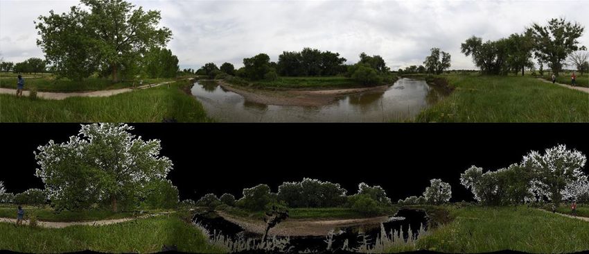
102                                                      S. Bywater-Reyes and B. Pratt-Sitaula: High-resolution topography course

planned for in-person implementation and were quickly re-                     This course and the activities it included contributed to
designed for remote delivery. Most US universities closed                  the NAGT Designing Remote Field Experiences collection
campuses in March 2020 and did not return to in person until               (https://serc.carleton.edu/NAGTWorkshops/online_field/
fall 2020 or later, whereas the field courses needed to occur              index.html, last access: 28 March 2022) (Egger et al.,
May through August 2020. In response to this crisis, geo-                  2021). The overall course is at https://serc.carleton.edu/
science field instructors worked together with the National                NAGTWorkshops/online_field/courses/240348.html          (last
Association of Geoscience Teachers (NAGT) to develop and                   access: 28 March 2022), and the individual activities are
share remote field teaching resources through the “Designing               linked within the course page, as well as contributing indi-
Remote Field Experiences” project (Egger et al., 2021).                    vidually to the “Teaching with Online Field Experiences”
   This paper describes one such impacted course that piv-                 collection        (https://serc.carleton.edu/NAGTWorkshops/
oted to remote teaching, “Geoscience Field Issues Us-                      online_field/index.html, last access: 28 March 2022).
ing High-Resolution Topography to Understand Earth Sur-
face Processes”, taught through the University of North-                   1.2   Value of course topic
ern Colorado (UNC). It was originally planned as an in-
person course with Structure from Motion photogrammetry                    High-resolution topographic datasets (SfM and ground-
(SfM), terrestrial laser scanning (TLS), and Global Naviga-                based and airborne lidar) are valuable in disciplines rang-
tion Satellite System (GNSS)1 data collection and analysis                 ing from geomorphology and tectonics to engineering and
applied to geomorphic issues in a mixed field and class-                   construction (Bemis et al., 2014; Passalacqua et al., 2015;
room setting. The course implementation and curriculum                     Robinson et al., 2017; Tarolli, 2014; Westoby et al., 2012).
were adjusted to a remote delivery mode by collecting TLS,                 Use of high-resolution data in Earth science education al-
GNSS, and uncrewed aerial system (UAS) imagery for SfM                     lows students to quantify landscapes and their change at sub-
prior to the course start. Informational videos about the                  meter resolution (Pratt-Sitaula et al., 2017; Robinson et al.,
field site and data collection were also provided to the stu-              2017). Understanding surface processes is listed as very im-
dents. The data were collected near Greeley, Colorado, on the              portant in the recent “Vision and Change in the Geosciences”
Cache la Poudre River by Bywater-Reyes from the Univer-                    with the objective “Students will be able to recognize key
sity of Northern Colorado, in collaboration with UNAVCO                    surface processes and their connection to geological features
(https://www.unavco.org/, last access: 28 March 2022).                     and possible natural and man-made hazards” (Mosher et al.,
Other geomorphic datasets were drawn from UNAVCO and                       2021, p. 17). Furthermore, use of multiple types of data al-
OpenTopography (https://opentopography.org/, last access:                  lows students to practice critical thinking skills such as as-
28 March 2022) archives. The class had 23 students in to-                  sessing which acquisition method is appropriate for different
tal (16 undergraduates and 7 graduate students).                           scenarios and what errors are associated with different meth-
   Bywater-Reyes was the primary course designer and in-                   ods. Critical thinking, integrating diverse data sources, and
structor for the course and led the adjustments to remote                  strong quantitative skills were all identified as very impor-
teaching. UNAVCO runs the National Science Foundation                      tant skills for undergraduate students to master (e.g., Kober,
(NSF) and National Aeronautics and Space Administration                    2015). Similarly, making inferences about the Earth system;
(NASA) geodetic facility (GAGE: Geodetic Facility for the                  making spatial and temporal interpretations; working with
Advancement of Geoscience). Its mission includes provid-                   uncertainty; and developing field, GIS, computational, and
ing educational support to the broader geodesy and geo-                    data skills were all listed as very important skills for geo-
science communities; thus, UNAVCO staff collaborated on                    science students to demonstrate (Mosher et al., 2021). Fur-
the prepared data collection. The teaching activities de-                  thermore, learning to collect, post-process, and analyze large
veloped for this course were adapted from UNAVCO’s                         datasets is a marketable transferable skill that prepares stu-
GEodesy Tools for Societal Issues (GETSI; https://serc.                    dents for the job market, with cartography and photogram-
carleton.edu/getsi/index.html, last access: 28 March 2022)                 metry job prospects being “excellent” according to the Bu-
modules: Analyzing High Resolution Topography with TLS                     reau of Labor Statistics. For historically marginalized stu-
and SfM (https://serc.carleton.edu/getsi/teaching_materials/               dents, high-paying job prospects are particularly important
high-rez-topo/index.html, last access: 28 March 2022) and                  (O’Connell and Holmes, 2011).
High Precision Positioning with Static and Kinematic GP-
S/GNSS (https://serc.carleton.edu/getsi/teaching_materials/                1.3   Value of remote learning to removing barriers
high-precision/index.html, last access: 28 March 2022)
                                                                           Fieldwork, while valuable to building students’ self-efficacy
   1 GNSS (Global Navigation Satellite System) is the general term         and problem-solving skills (Elkins and Elkins, 2007), can
that refers to all Earth’s satellite navigation systems. Most peo-         pose a barrier to diversifying the geosciences because of
ple are more familiar with the term GPS (Global Positioning Sys-           ableism (Carabajal and Atchison, 2020), cost (Abeyta et
tem), which, technically, only refers to the US satellite constellation.   al., 2020), cultural factors (Hughes, 2015), racism (Ab-
Hereafter, this paper will refer to GNSS or GPS/GNSS.                      bott, 2006), and sexism (Fairchild et al., 2021) in the field.

Geosci. Commun., 5, 101–117, 2022                                                               https://doi.org/10.5194/gc-5-101-2022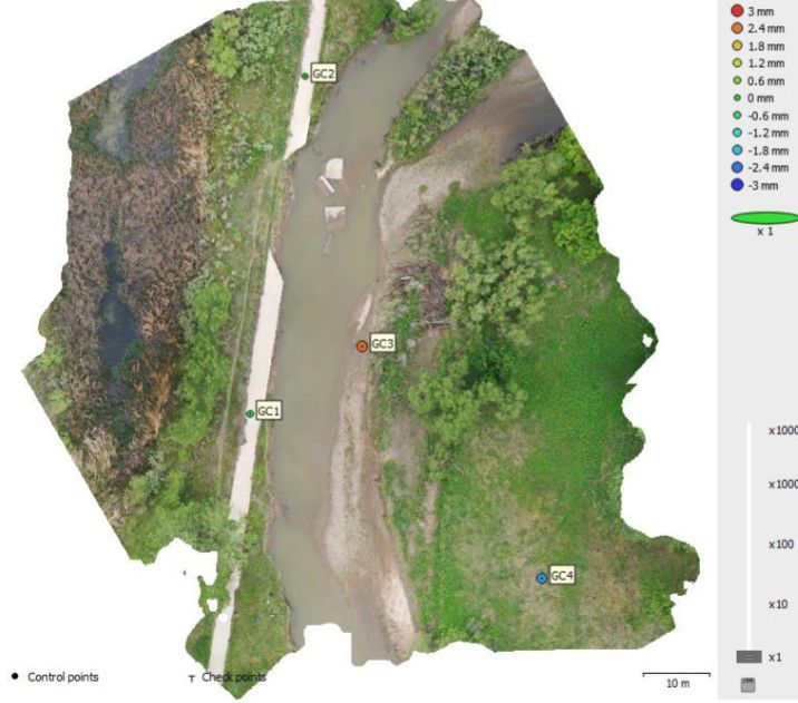
S. Bywater-Reyes and B. Pratt-Sitaula: High-resolution topography course                                                  103

COVID-19 forced the geosciences to develop virtual field         between. The bulk of the instruction occurred within a 2-
experiences, with a positive side effect of removing many        week period during the summer. Synchronous lectures were
of the aforementioned barriers to fieldwork completion. For      conducted via Zoom and course content distributed via Can-
example, the computer-based nature of remote field learning      vas. The class used Slack as an asynchronous way to ex-
removes many physical accessibility issues present for typi-     change questions, comments, and solutions amongst the stu-
cal field courses. The option to learn from home may make        dents and between the students and instructor. During the
the remote courses more feasible for students with family or     course, students worked with three different analytical soft-
work responsibilities, as well as reducing real and perceived    ware packages: Agisoft MetaShape, CloudCompare, and Ar-
safety issues related to gender, sexual orientation, and race    cGIS Map. Five students attended an optional in-person field
that may occur in tradition field camp settings. Although re-    collection campaign (one student traveled from out of state,
mote field courses are not necessarily the most desirable for    and the remainder were UNC students). The course was di-
all students, the development of high-quality remote field op-   vided into two units: Unit 1 focused on the SfM workflow,
tions can be one component of diversifying the geosciences       including integrating GNSS and point cloud processing, and
(Egger et al., 2021).                                            Unit 2 on lidar products and workflows, including TLS, topo-
                                                                 graphic differencing, airborne lidar, and method comparison.
                                                                 Each unit ended in a unit report, with the second providing
2     Course overview and learning outcomes
                                                                 students an opportunity to improve workflows and explore
2.1    Course objectives and geodetic methods
                                                                 additional data sources and analyses.

The objective of the course was for students to learn man-       2.3   Learning outcomes
ual and remote sensing methods of topographic data collec-
tion, including (1) GPS/GNSS, (2) SfM, and (3) TLS sur-          The course-specific learning outcomes were that students
veying and airborne lidar use. GNSS uses ground-based re-        should be able to do the following:
ceivers to trilaterate positions calculated from signals sent
                                                                  A. Make necessary calculations to determine the optimal
by orbiting satellites (to accuracies of a couple of centime-
                                                                     survey parameters and survey design based on site and
ters in this use case). SfM is a photogrammetric technique
                                                                     available time.
that uses overlapping images to construct three-dimensional
models with widespread research applications in geodesy,          B. Integrate GNSS targets with ground-based lidar and
geomorphology, structural geology, and other subfields in the        SfM workflows to conduct a geodetic survey.
geosciences (Passalacqua et al., 2015; Westoby et al., 2012).
Lidar also generates three-dimensional models valuable for        C. Process raw point cloud data and transform a point
the same range of applications, but it uses laser scanners to        cloud into a digital elevation model (DEM).
send out thousands of laser pulses per second, measure the        D. Conduct an appropriate geomorphic analysis, such as
return time, and calculate distances. Scanners can be ground-        geomorphic change detection.
based (TLS) or airborne. SfM requires less expensive equip-
ment and less field time but more processing time than TLS.       E. Justify which survey tools and techniques are most ap-
In low-vegetation field areas, SfM can yield similarly valu-         propriate for a scientific question.
able high-resolution topographic models with point densities
usually hundreds of points per square meter (depending on        The course activities also helped students meet many of
instrument-to-object distance; Westoby et al., 2012); how-       the NAGT learning outcomes for capstone field experi-
ever, TLS is much more effective in areas with dense vegeta-     ences. These nine outcomes were developed by a group
tion. For both methods, ground control points (GCPs), usu-       of 32 experienced field educators, who came together
ally measured with GNSS, are needed for georeferencing the       in spring 2020 to develop comprehensive learning out-
topographic model. For SfM, they are also critical for reduc-    comes for field experiences that are relevant to both in-
ing distortions and errors (James et al., 2019). One of the      person or online delivery modes (https://serc.carleton.edu/
key outcomes for students was to understand the benefits and     NAGTWorkshops/online_field/learning_outcomes.html, last
challenges of each method and how to determine the most          access: 28 March 2022). By the end of a capstone field ex-
valuable in different circumstances.                             perience, whether that experience is online or in person, stu-
                                                                 dents should be able to do the following:

2.2    Course delivery                                            1. Design a field strategy to collect or select data in order
                                                                     to answer a geologic question.
Course content focused on Earth-surface process applica-
tions but could be adapted to other geoscience topics. The        2. Collect accurate and sufficient data on field relation-
course was taught workshop-style, composed of multiple               ships and record these using disciplinary conventions
synchronous work sessions with asynchronous work time in             (field notes, map symbols, etc.).

https://doi.org/10.5194/gc-5-101-2022                                                  Geosci. Commun., 5, 101–117, 2022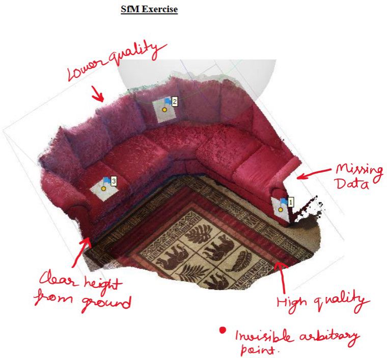
104                                              S. Bywater-Reyes and B. Pratt-Sitaula: High-resolution topography course

 3. Synthesize geologic data and integrate with core con-        2015). Near Greeley, significant portions of the Poudre Trail
    cepts and skills into a cohesive spatial and temporal sci-   were impacted as the river topped its floodplain and eroded
    entific interpretation.                                      its banks. The study site is adjacent to the Poudre Trail, with
                                                                 portions of the former trail eroded into the river and the cur-
 4. Interpret Earth systems and past, current, and future pro-   rent trail rerouted around the 2013-developed river course.
    cesses using multiple lines of spatially distributed evi-       Data for student use were collected from the Poudre River
    dence.                                                       by a joint UNAVCO-UNC team in May 2020. The types of
                                                                 data included were as follows:
 5. Develop an argument that is consistent with available
    evidence and uncertainty.                                        – UAS-collected photographs for SfM point cloud gener-
                                                                       ation (DJI Mavic 2 Pro)
 6. Communicate clearly using written, verbal, and/or vi-
    sual media (e.g., maps, cross-sections, and reports) with        – point clouds collected using TLS (Riegl VZ400)
    discipline-specific terminology appropriate to your au-
    dience.                                                          – several hours of GNSS base station data (Septentrio Al-
                                                                       tus APS3G)
 7. Work effectively, independently, and collaboratively
    (e.g., commitment, reliability, leadership, openness for         – GNSS-measured ground control point locations for geo-
    advice, channels of communication, support, and inclu-             referencing both SfM and TLS surveys (Septentrio Al-
    sion).                                                             tus APS3G)

 8. Reflect on personal strengths and challenges (e.g., in           – videos of field site and field methods.
    study design, safety, time management, and indepen-
    dent and collaborative work).                                3    Methods
 9. Demonstrate behaviors expected of professional geosci-       This course was developed and implemented in response to
    entists (e.g., time management, work preparation, colle-     the COVID-19 pandemic and the need for students to ful-
    giality, health and safety, and ethics).                     fill degree requirements and not designed as an educational
Table 1 shows the alignment between the daily activities and     research study before implementation. Thus, there are in-
course-specific and NAGT learning outcomes. It also pro-         herent limitations to the available data and conclusions that
vides links to the activity pages within the NAGT Teaching       can be drawn from the project. Nonetheless, there is value
with Online Field Experiences collection.                        in sharing this robust open-source curriculum, describing
                                                                 how the course was implemented and outlining how student
                                                                 learning outcomes were assessed and achieved. This study
2.4   Field site and prepared data                               went through the Institutional Review Board at University of
The course field site was the Cache la Poudre River at           Northern Colorado, which determined this project to be ex-
Sheep Draw Open Space (City of Greeley Natural Areas)            empt under 45 CFR 46.104(d)(704) for research, Category 4.
in northern Colorado. It was selected for the following rea-     Therefore, course artifacts and student demographic data can
sons: (1) the site shows both standard river features and ev-    be used in research so long as no identifying information is
idence of extreme flooding, (2) the Poudre River is impor-       revealed. Student artifacts included submitted assignments,
tant to several local communities, and (3) the site is proxi-    unit reports, posts from a daily Slack discussion forum and
mal to the UNC campus. According to the Coalition for the        unsolicited feedback given directly to the instructor. We ex-
Poudre River Watershed, “The Cache la Poudre River Wa-           tracted examples from artifacts and associated assessments
tershed drains approximately 2.735 E9 m2 above the canyon        to illustrate students’ accomplishments and evaluate whether
mouth west of Fort Collins, Colorado. The watershed sup-         the course and, to a lesser extent, NAGT learning outcomes
ports the Front Range cities of Fort Collins, Greeley, Tim-      for capstone field experiences were met. We describe the
nath and Windsor. In an average year, the watershed pro-         Course implementation and assessment approach in Sect. 4
duces approximately 3.38 E8 m2 of water. More than 80 %          and alignment with course-specific (Sect. 5.1) and other out-
of the production occurs during the peak snowmelt months         comes (Sect. 5.2) in Sect. 5. We finish with Lessons learned
of April through July” (https://www.poudrewatershed.org/         and implementation recommendations in Sect. 6.
cache-la-poudre-watershed, last access: 28 March 2022). In
2013, the Front Range and plains of Colorado experienced         4    Course implementation and assessment approach
extensive flooding. The region received the average annual
rainfall in 1 week (Gochis et al., 2015). There was extensive    This section gives a brief overview of each course activity
damage to infrastructure and in some cases the erosion of a      (Table 1) and which course-specific learning outcomes and
1000 years’ worth of weathered material (Anderson et al.,        NAGT outcomes are at least partially addressed. Table 2 is

Geosci. Commun., 5, 101–117, 2022                                                      https://doi.org/10.5194/gc-5-101-2022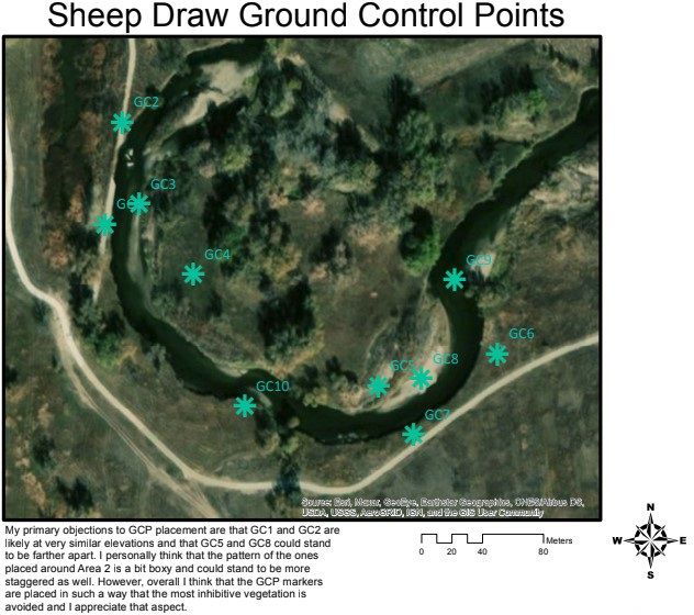
S. Bywater-Reyes and B. Pratt-Sitaula: High-resolution topography course                                                              105

Table 1. Activities by day and alignment with course-specific and NAGT learning outcomes.

         Activity                                                                      Course-specific learning      NAGT capstone
                                                                                       outcomes                      field learning
                                                                                                                     outcomes
         Course Unit 1: SfM and GPS/GNSS                                               A. Survey design              1, 2, 7
         Day 1 – Getting started with Structure from Motion (SfM) photogrammetry       C. Point cloud and DEM
         (https://serc.carleton.edu/NAGTWorkshops/online_field/activities/238996.
         html, last access: 28 March 2022)
         Day 2a – GPS/GNSS Fundamentals (https://serc.carleton.edu/getsi/              A. Survey design              1
         teaching_materials/high-precision/unit1.html, last access: 28 March 2022)     B. GNSS and geodetic
                                                                                       survey
                                                                                       E. Justify tools and tech-
                                                                                       niques
         Day 2b – Post-processing GPS/GNSS Base Station Position (https://serc.        B. GNSS and geodetic          1
         carleton.edu/NAGTWorkshops/online_field/activities/239147.html, last ac-      survey
         cess: 28 March 2022)
         Day 3a – Ground Control Points for Structure from Motion activity (https:     A. Survey design              1–5, 7, 9
         //serc.carleton.edu/NAGTWorkshops/online_field/activities/239349.html,        B. GNSS and geodetic
         last access: 28 March 2022)                                                   survey
         Day 3b – Structure from Motion for Analysis of River Characteristics          C. Point cloud and DEM        1–5
         activity (https://serc.carleton.edu/NAGTWorkshops/online_field/activities/    D. Geomorphic analysis
         239350.html, last access: 28 March 2022)
         Day 4 – Working with Point Clouds in CloudCompare and Classi-                 C. Point cloud and DEM        3–5
         fying with CANUPO (https://serc.carleton.edu/NAGTWorkshops/online_            D. Geomorphic analysis
         field/activities/240357.html, last access: 28 March 2022)                     E. Justify tools and
                                                                                       techniques
         Day 5 – SfM Feasibility Report assignment (https://d32ogoqmya1dw8.            A. Survey design              3–6
         cloudfront.net/files/NAGTWorkshops/online_field/courses/sfm_                  B. GNSS and geodetic
         feasibility_report.v2.docx, last access: 28 March 2022)                       survey
                                                                                       C. Point cloud and DEM
                                                                                       D. Geomorphic analysis
                                                                                       E. Justify tools and tech-
                                                                                       niques
         Day 6 – Optional field day                                                    B. GNSS and geodetic          1, 7, 9
                                                                                       survey
         Course Unit 2: TLS, Topographic Differencing, and Method Compari-             C. Point cloud and DEM        3–7, 9
         son Day 7 – Introduction to terrestrial laser scanning (TLS) (https://serc.   (E. Justify tools and tech-
         carleton.edu/NAGTWorkshops/online_field/activities/241028.html, last ac-      niques)
         cess: 28 March 2022)
         Day 8a – Point Cloud and Raster Change Detection (https://serc.               C. Point cloud and DEM        3–7, 9
         carleton.edu/NAGTWorkshops/online_field/activities/241083.html, last ac-      E. Justify tools and tech-
         cess: 28 March 2022)                                                          niques
         Day 8b – DEM of Difference (https://serc.carleton.edu/NAGTWorkshops/          C. Point cloud and DEM        3–7, 9
         online_field/activities/241138.html, last access: 28 March 2022)              D. Geomorphic analysis
         Day 9 – OpenTopography Data Sources and Topographic Differ-                   C. Point cloud and DEM        3–6, 9
         encing (https://serc.carleton.edu/NAGTWorkshops/online_field/activities/      D. Geomorphic analysis
         241410.html, last access: 28 March 2022)
         Day 10 – Method Comparison Report                                             A. Survey design              3–6
         (https://d32ogoqmya1dw8.cloudfront.net/files/NAGTWorkshops/                   C. Point cloud and DEM
         online_field/courses/methods_comparison_report.docx,  last         access:    D. Geomorphic analysis
         28 March 2022)                                                                E. Justify tools and tech-
                                                                                       niques
         Day 11 – Presentations                                                        D. Geomorphic analysis        6–7, 9
                                                                                       E. Justify tools and tech-
                                                                                       niques

https://doi.org/10.5194/gc-5-101-2022                                                               Geosci. Commun., 5, 101–117, 2022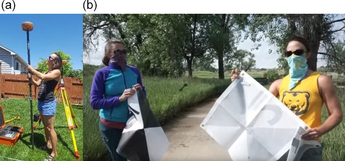
106                                              S. Bywater-Reyes and B. Pratt-Sitaula: High-resolution topography course

an example of the type of rubric used in grading simple stu-     4.2   Day 2: Introduction to GPS/GNSS
dent assignment answers, such as in daily assignments, with
                                                                 In the Day 1 activity, students used a relative local coordi-
discretion used to assign percentages within these ranges.
                                                                 nate system to produce an accurately scaled model. However,
Most questions also had the points possible indicated so that
                                                                 for real-world applications a global coordinate system is fre-
students could gauge their relative significance towards the
                                                                 quently preferable, which can be achieved with survey-grade
grade. Multi-component rubrics were used for more in-depth
                                                                 GPS/GNSS, so Day 2 was focused on course outcomes A
exercises, such as unit reports. In such cases, students were
                                                                 (survey design), B (GNSS and geodetic survey), and E (jus-
informed of the weighted percent for each section (e.g.,
                                                                 tifying techniques). Day 2 morning activities were adapted
title, abstract, and introduction) and also given a detailed
                                                                 from the GETSI module High Precision Positioning with
description of what should be included in each (https:
                                                                 Static and Kinematic GPS/GNSS. First, students learned
//d32ogoqmya1dw8.cloudfront.net/files/NAGTWorkshops/
                                                                 about the method through a lecture. Next, they worked with
online_field/courses/sfm_feasibility_report.v2.docx,      last
                                                                 data collected using different types of receivers and result-
access: 28 March 2022). The same simple rubric (Table 2)
                                                                 ing accuracy and precision. Assessment included a concept
was used to assess each weighted section. For example, the
                                                                 sketch of GPS/GNSS systems, quantification and evaluation
Discussion section was weighted 20 %, and students were
                                                                 of accuracy and precision of different grades of GNSS, and
instructed as follows:
                                                                 recommendations for appropriate applications of each.
      Here, you can discuss both pros and cons of                   In the afternoon of Day 2, students were introduced to the
      the methods (What worked? Didn’t work? What                field site and methods used for data collection at the Cache la
      would improve the workflow?) as well as what               Poudre field location (described above in Sect. 2). Students
      you discovered about the Poudre River at the site.         watched a video (Video 1; https://youtu.be/EZ5I8Ge8YjI,
      Return to the question of feasibility. Consider the        last access: 28 March 2022) about the field site and a video
      overall goal of using SfM to assess geomorphic             introducing the GNSS methods (Video 2; https://youtu.be/
      processes on the Poudre River at Sheep Draw. How           Xpj1QJf8AkY, last access: 28 March 2022). Then, using the
      could SfM be applied? What are the limitations?            pre-collected base-station data, students completed the Post-
                                                                 Processing GPS/GNSS Base Station Position assignment.
  Similarly detailed instructions accompanied all compo-         Students submitted the base station file to the Online Posi-
nents for the more in-depth exercises.                           tioning User Service (OPUS), the National Geodetic Survey
                                                                 (NGS)-operated system for baseline processing of standard-
4.1   Day 1: Getting started with Structure from Motion          ized RINEX files into fixed (static) positions. For the assess-
      (SfM) photogrammetry                                       ment, students wrote a paragraph explaining their procedure,
                                                                 interpreting the results, describing the difference between el-
Course Unit 1: SfM and GPS/GNSS started out on Day 1
                                                                 lipsoid height and orthometric height, and highlighting any-
with an introduction to the SfM method. The day’s activ-
                                                                 thing that was surprising or confusing about the results.
ities were the first step in addressing course outcomes A
(survey design) and C (point cloud data). After an overview
presentation, students used smartphone cameras to take ∼         4.3   Day 3: SfM of Poudre River at Sheep Draw Reach
20 overlapping photos of an object of interest (e.g., sofa,      On Day 3 students combined skills learned in the previous
shed, or berm). For simplicity and to learn about local ref-     2 d in order to create a georeferenced point cloud from the
erence frames (rather than global ones from GNSS), they          field site (course outcomes A–C) and started to consider rel-
took compass bearing, inclination, and distance measure-         evant geomorphic analyses (outcome D). The morning exer-
ments and used trigonometry to calculate x–y–z coordinates       cise was “Ground Control Points for SfM” at the Cache la
for the ground control points (GCPs). Students used Agisoft      Poudre site. This began with a group discussion on where
MetaShape software to post-process their photos and create       ground control points at the site should be placed within the
the 3D point clouds. The software was available on their per-    field area (Fig. 1). Students were then given a text file of the
sonal computers through a 30 d trial licence. Students then      x, y, and z coordinates (UTM) collected by the UNAVCO-
evaluated the performance of their model by considering data     UNC team, and had to import them into ArcGIS to create
quality in different model regions and what method changes       a ground control point map. In a follow-up discussion, stu-
might improve their product. They also made recommenda-          dents compared the ground control point locations actually
tions for how SfM could be applied to different fields in the    used in the prepared data with the locations they discussed
geosciences. The assessment of student learning was based        for placement in the initial discussion. They were asked to
on successful production of a locally referenced point cloud     summarize the strengths and weaknesses of the implemented
and the data quality analysis.                                   ground control point plan at the site, which helped to assess
                                                                 learning related to both survey design outcomes.

Geosci. Commun., 5, 101–117, 2022                                                     https://doi.org/10.5194/gc-5-101-2022
S. Bywater-Reyes and B. Pratt-Sitaula: High-resolution topography course 107
Table 2. Example rubric showing percentage scoring used to assess course activities.
Exemplary (75 %– Basic (50 %– Minimal effort (25 %– Nonperformance
100 % points) 75 % points) 50 %) (0 %–25 %)
General Exemplary work will not Basic work may answer all Minimal performance oc- Nonperformance occurs
considerations just answer all compo- components of the given curs when student answers when students are missing
nents of the given question question, but answers are simply do not make sense large portions of the as-
but also answer correctly, incorrect, ill-considered, or and are incorrect. signment.
completely, and thought- difficult to interpret given
fully. Attention to detail, the context of the question.
as well as answers that are Basic work may also be
logical and make sense, is missing components of a
an important piece of this. given question.
control point network used. Finally, students were asked to
formulate a testable hypothesis related to processes on the
Cache la Poudre River that they could answer with their
dataset. For example, students could investigate cutbank sta-
ble bank heights and angles. The completed exercise was the
summative assessment and particularly revealed student ac-
complishment of SfM point cloud creation and geomorphic
analysis.
4.4 Day 4: Using CloudCompare and classifying with
CANUPO
On Day 4, students used the open-source software
CloudCompare (http://www.danielgm.net/cc/, last access:
28 March 2022), which allows for the viewing and manip-
ulation of point clouds. This was a continuation of the same
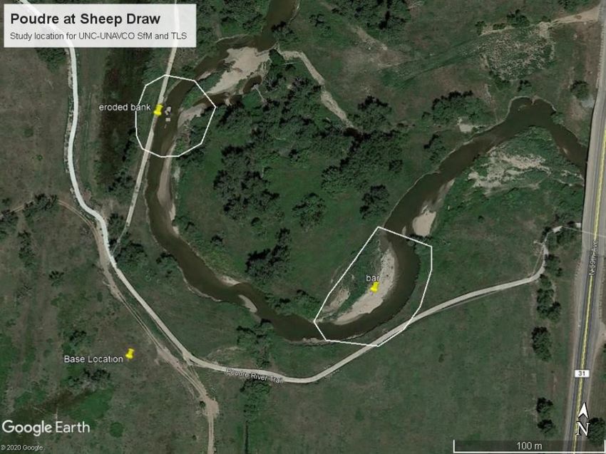
Figure 1. Inset: Map (© Google Earth) of the Cache la Poudre River learning outcomes as the afternoon of Day 3 (outcomes C
Watershed, located in northern Colorado, United States. The study and D) and continued on to some justification of methods
site at Sheep Draw has two areas of interest, Area of Interest 1 on (outcome E). Students learned the basic operations used in
an eroded bank and Area of Interest 2, a cutbank and point bar. CloudCompare, such as importing point clouds, classifying
the points, and taking measurements that allow for hypoth-
esis testing. They also incorporated an open-source plug-
The afternoon exercise was the “Structure from Motion in called CANUPO (http://nicolas.brodu.net/en/recherche/
for Analysis of River Characteristics”. Students picked ei- canupo/, last access: 28 March 2022) that facilitates addi-
ther Area of Interest 1 or 2 for their SfM workflow (Fig. 1). tional point cloud classification (Brodu and Lague, 2012),
Students with adequate computing power could choose to do such as distinguishing between vegetation and ground. Stu-
the entire study region. Using resolution and height infor- dents create a digital elevation model (DEM) from ground
mation about the UAS-collected photographs, students first points and export it for use in ESRI ArcGIS Map. In Ar-
calculated the expected resolution of the final point cloud. cGIS, students familiarized themselves with viewing 3D data
They were then asked to assess what types of features or pro- in 2.5D and created hillshade and slope maps. Then they
cesses at the Cache la Poudre study area they expected could were asked to retest their hypothesis with tools available in
be resolved; from there, they discussed the types of geomor- ArcGIS and 2.5D (e.g., measure tool and raster values). Stu-
phic questions they could feasibly expect to answer with the dents compared and contrasted applications with the three-
dataset of that resolution. Next, students followed a more de- dimensional point cloud versus 2.5D raster and summarized
tailed Agisoft MetaShape guide to construct a georeferenced the appropriate uses and applications of each in the day’s as-
point cloud of their area of interest. As they were familiar signment.
with MetaShape from Day 1, students were able to work
through the procedure independently. Once their model was
complete, students were asked to answer a series of questions
related to error analysis of their model and to reassess ap-
propriate geomorphic applications and design of the ground
https://doi.org/10.5194/gc-5-101-2022 Geosci. Commun., 5, 101–117, 2022108 S. Bywater-Reyes and B. Pratt-Sitaula: High-resolution topography course
4.5 Day 5: SfM Feasibility Report assignment
The summative assessment for Course Unit 1 was the SfM
Feasibility Report, which included assessment of all five
course outcomes. Students were to imagine themselves as
natural resource managers and assigned the task of inves-
tigating the feasibility of using SfM to study geomorphic
processes on the Cache la Poudre River. They were asked
to summarize the SfM workflow and present the outcomes,
limitations, and suggested applications of their SfM model of
their Poudre area of interest. On Day 5, students were given
Figure 2. Base and kinematic GNSS methods (a) and example of
a work day to complete the report.
ground control (b) surveyed for use in GNSS and SfM activities.
4.6 Day 6: Optional field trip
Day 6 consisted of an optional field demonstration dur- TLS data for their area of interest using CloudCompare with
ing which students completed a GNSS ground con- the M3C2 Plugin (Lague et al., 2012). Since these datasets
trol survey, and Bywater-Reyes and colleagues collected were collected at the same place on the same day, differences
UAS images at the Poudre Learning Center (https://youtu. between the datasets were due to errors or uncertainties in
be/s5CGhk8GIOUBrodu; Bywater-Reyes, Sharon: Poudre one or both of the models. Students were asked to interpret
Learning Center Project. https://doi.org/10.5446/54388). the 3D differences between the datasets. The second lecture,
on raster differencing, discussed best practices in preparing
rasters for differencing (Wheaton et al., 2010). Students then
4.7 Day 7: Introduction to terrestrial laser scanning used the ArcGIS Raster Calculator tool to subtract one raster
(TLS) from the other. Students interpreted the results and compared
Day 7 was the start of Course Unit 2: TLS, Topographic the differences between 3D (point cloud) and 2.5D (raster)
Differencing, and Method Comparison and began with an differencing. The summative assessment was the assignment
introduction to TLS methodology through a video and lec- in which students interpreted their results as an error analy-
ture. The exercise used pre-collected TLS data that the stu- sis and discussed which dataset they think is more accurate
dents were asked to compare and contrast with the SfM point (and why) and which method provided the most robust error
cloud they had developed in Unit 1, which was collected analysis.
from the same geographic location (Cache la Poudre River) So that the students could gain experience with airborne
on the same day (Fig. 3). The learning outcomes primarily fo- lidar data and with actual geomorphic change detection, dur-
cused on outcome C (point clouds) but also laid the ground- ing the afternoon of Day 8 they were given two lidar-derived
work for more advanced method comparison to come (out- raster datasets collected before and after the 2013 floods of
come E). Students visually inspected the datasets for simi- the Colorado Front Range on a river (South St. Vrain Creek)
larities and differences; then they measured geomorphic fea- that experienced substantial geomorphic change. In the ex-
tures in the scene and compared their measurements for the ercise “DEM of Difference”, students practiced raster dif-
two methods. Using skills gained in previous class activities, ferencing skills in the context of geomorphic change detec-
students classified the TLS cloud into vegetation and ground, tion and also characterized their detection limit with a simple
exported the ground cloud as a text file, and created a raster thresholding approach. This helped to further address out-
that matched the specifications of the one made in the SfM comes C and D as students answered questions in the as-
activity. This prepared for 3D (cloud-to-cloud differencing) signment about the differencing method and made a series of
and raster differencing on Day 8. Assessment (mostly forma- calculations that pertained to geomorphic change.
tive) was based on their completion of measurements and a
discussion of method comparison, including a group discus- 4.9 Day 9: OpenTopography data sources and
sion. topographic differencing
To broaden student knowledge of data availability, Day 9
4.8 Day 8: Point cloud/raster differencing and change
focused on additional high-resolution (usually lidar) data
detection
sources. After a lecture, students conducted an assignment
On the morning of Day 8, students used the concepts of point using existing high-resolution datasets housed within Open-
cloud and raster differencing to further compare their SfM Topography (OT; https://opentopography.org/, last access:
and TLS results and interpret differences between the meth- 28 March 2022). First, students practiced downloading and
ods (outcomes C and E). After a lecture on point cloud differ- viewing data from OT; second students conducted a topo-
encing, students proceeded with differencing of the SfM and graphic differencing exercise (Crosby et al., 2011), comple-
Geosci. Commun., 5, 101–117, 2022 https://doi.org/10.5194/gc-5-101-2022S. Bywater-Reyes and B. Pratt-Sitaula: High-resolution topography course 109
Figure 3. The top shows the terrestrial laser scanner photograph from a scan location, whereas the bottom shows the associated point cloud
at the Cache la Poudre River site. Courtesy of UNAVCO.
menting the point cloud and raster differencing students con- 5.1.1 (A) Make necessary calculations to determine the
ducted on Day 8. As with the afternoon of Day 8, the learning optimal survey parameters and survey design
outcomes primarily focused on point clouds and geomorphic based on site conditions and available time
analysis (C and D). The learning assessment was done via
the student assignment, in which students determine erosion In the GNSS/GPS accuracy and precision activity (Day 2),
and deposition in a dune field and analyze error and detection students showed their ability to evaluate appropriate GP-
thresholds. S/GNSS techniques in different contexts with the GPS/GNSS
error analysis activity (Day 2). Students calculated and com-
4.10 Days 10 and 11: Method Comparison Report and pared accuracy and precision of different GNSS/GPS meth-
presentation ods and (Day 2) explained which types of surveys or re-
search applications are appropriate for each. Students re-
The summative assessment for Course Unit 2 and the course ceived an average of an 89 % of this assignment (exemplary),
as a whole was the final “Method Comparison Report” and evidence of their ability to link calculations to applications.
presentations in the last 2 d of the course. Students picked Students also completed a concept sketch of GNSS systems
from a variety of options including improving methods from (Fig. 4) describing what factors can interfere with GNSS per-
Unit 1 (SfM and TLS methods), adding new elements to formance.
Unit 1, choosing an additional exploration with the datasets In the SfM activity (Day 3), students calculated the pixel
collected on the optional field day, or using a different dataset resolution resulting from the flight parameters used in the
such as airborne lidar. As the course summative assessment, pre-collected UAS images and assessed the appropriateness
the report pulled together student learning on all five course of this resolution to resolve features within the flight. One
outcomes. The presentation (Day 11) additionally gave stu- student wrote in their assignment, “Obviously the larger scale
dents practice in oral presentation of scientific findings. features will be resolved, like the eroded bank, point bar,
and the sidewalk panels in the river, as well as most sizes
5 Results of vegetation. If the sampling is 0.3–0.5 cm per pixel, then
it should be able to resolve grasses, and just about any size
5.1 Course-specific learning outcomes of gravel. The difference between the water surface and ad-
jacent should be pretty well resolved as well.” They were
This section provides a variety of examples of how students
also given the UAS flight time for the survey. Thus, stu-
met the different course-specific learning outcomes. It is not
dents could easily adapt this approach to calculate the time it
intended to be exhaustive but to provide general illustrations
would take to accomplish a flight reaching the desired reso-
of student learning drawn from both assignments and Slack
lution for a given application. The discussion of implemen-
daily reflections and discussions.
tation of ground control at the field site (Day 3) allowed stu-
dents to compare the actual implementation with literature-
recommended protocols to discuss strengths and weaknesses
given the site conditions (Fig. 5). Students also showed the
ability to discern improvements to the survey plan given the
https://doi.org/10.5194/gc-5-101-2022 Geosci. Commun., 5, 101–117, 2022110 S. Bywater-Reyes and B. Pratt-Sitaula: High-resolution topography course
Figure 4. Student sketch of how GNSS works, including disruptions and applications thereof demonstrating theoretical understanding of
GNSS (created by student in course for Day 2 activity; student name not disclosed to comply with Institutional Review Board).
site condition. For example, one student wrote: “I think the students did integrate GNSS targets with an SfM workflow
GCPs [ground control points] are very well placed in area-1 to conduct a geodetic survey, they did not actively integrate
and area-2. But the adjoining area of both the areas only got GNSS targets for the TLS workflow. The lack of TLS target
two GCPs – GC4 and GC10 which is too [few]. It may reduce integration stemmed from the remote nature of the course
the accuracy of map while joining area-1 and area-2. In addi- and pre-collected nature of the field campaign, whereas an
tion, area-2 has only one GCP in North direction which may in-person implementation would have allowed students to be
become an issue during georeferencing. To be on safer side actively involved with TLS target GNSS data collection and
we may include one more GCP near GC9 to ensure the cover- integration. Future remote implementations would need an
age of area-2. If only 9 GCPs are available to me then I think activity that involves students in TLS GNSS target data col-
the current arrangement of GCP is best.” Students received an lection and post-processing to meet this learning outcome.
average of 98 % (exemplary) on this discussion, highlighting However, given the complicated nature of TLS data post-
their ability to evaluate appropriate methods given site con- processing, the authors recommend a simple activity such as
ditions. a discussion of recommended scan locations and a compari-
son of actual GNSS target locations compared to the recom-
mendation (e.g., similar to that conducted for the SfM field
5.1.2 (B) Integrate GNSS targets with ground-based
project). In a virtual course format, this learning outcome
lidar and SfM workflows to conduct a geodetic
would need to be edited in the future.
survey
Students used pre-collected GNSS-measured ground con- 5.1.3 (C) Process raw point cloud data and transform a
trol points to georeference the resulting SfM point cloud in point cloud into a digital elevation model (DEM)
the Day 3 SfM activity. As described in the previous sec-
tion (Sect. 5.1.1), students integrated the GNSS data into the Students practiced and successfully converted raw point
SfM projects and also discussed the overall survey design clouds to DEMs several times (Day 4 and Day 7) and also
and resulting model errors. The suite of activities that used learned how to use the native MetaShape point cloud classi-
pre-collected GNSS data was successful as indicated by as- fication (Day 3) as well as the open-source CANUPO (Day 4)
sessment data and student discussions (Sect. 5.1.1). Whereas version. When comparing point cloud versus raster eleva-
Geosci. Commun., 5, 101–117, 2022 https://doi.org/10.5194/gc-5-101-2022S. Bywater-Reyes and B. Pratt-Sitaula: High-resolution topography course 111
Figure 5. Student map of ground control points (GCPs) used in SfM activity (created by student in course; student name not disclosed to
comply with Institutional Review Board). Through a group discussion on Day 2, students discussed whether GCPs were adequately placed
and suggested implementation improvements. Imagery source: ArcGIS® software by Esri.
tion products, a student wrote: “It was hypothesized that SfM peat a workflow originally implemented over several days in
methodologies would be best at providing measurements of one step independently to produce a DEM.
large-scale elevation changes, however the clear decrease in
point cloud density decreased our confidence in these large-
5.1.4 (D) Conduct an appropriate geomorphic analysis,
scale elevation change measurements along the bank. Small-
such as geomorphic change detection
scale elevation changes along the point bar were best rep-
resented by the ArcMap generated hillshade map and DEM With the SfM and TLS field datasets, students recognized the
while large-scale elevation changes were best represented by limitation of having only one time snap. A student reported:
the ArcMap generated slope map and DEM. The slope map “Structure from motion to assess geomorphic processes on
also had the unique feature of highlighting areas of constant the Poudre River at Sheep Draw is useful and easy to op-
slope and could be used to distinguish between man-made erate. In this project we used SfM to create a model that
structures and natural vegetation areas in a site of flood dam- can measure bank erosion and deposition. However, we did
age.” Here, the student showed their ability to recognize pros not have enough information to analyze the rate at which the
and cons of point cloud versus raster (DEM) products. Stu- river was eroding the bank. To conduct this study we would
dents received an average of 84 % (exemplary) on the raster need to conduct several SfM surveys over a length of time
derivation and manipulation assignment and did even better to acquire enough variance in data to calculate a rate.” This
when they repeated this process. Students received an aver- statement illustrates the student’s recognition of the utility
age of 89 % (exemplary) on the TLS assignment, where they of repeat topographic data needed to conduct a geomorphic
were asked to repeat the process of conducting a quantita- change analysis that would be appropriate to answer a geo-
tive analysis on the cloud, classify the point cloud, extract morphic question they had posed.
ground points, and create a DEM, showing their ability to re- In the context of comparing SfM and TLS data collected
at the field site at the same time, students conducted point
https://doi.org/10.5194/gc-5-101-2022 Geosci. Commun., 5, 101–117, 2022112 S. Bywater-Reyes and B. Pratt-Sitaula: High-resolution topography course
cloud and raster differencing (Day 8). Students received an
average score of 78 % (low-end of exemplary) on this as-
signment and extrapolated how one could apply these meth-
ods to geomorphic change detection. A student noted in their
daily Slack discussion that “learning about DoD [DEM of
Difference] was a little confusing to me and some of the as-
signment parts threw me off but other than that I felt like I
learned good things today!” Another student said that “To-
day’s work was a lot more confusing than the last couple
days, but it’s much more satisfying.” Students illustrated their
enthusiasm for manipulated point clouds. A student wrote in
their daily discussion, “Today I enjoyed getting visible prod-
ucts using ArcMap and CloudCompare.” In comparing the
SfM and TLS datasets, a student demonstrated their under-
standing of how the differencing would be used in the context
of geomorphic change by stating: “During geomorphological
analysis, magnitude and direction are both important. Areas
that are positive show deposition, while negative areas show
erosion.”
Students conducted lidar geomorphic change detection
Figure 6. Student SfM product from Day 1 exercise (created by
with the Day 8 afternoon activity using regional lidar from
student in course; student not disclosed to comply with Institutional
Colorado 2013 floods and Day 9 (OpenTopography change
Review Board). Student successfully assessed relative data quality
detection). Students received the lowest assignment scores as indicated by student’s markup and where data were missing or of
on these, with 50 % and 75 %, respectively (basic to minimal low quality.
performance level). This may indicate a combination of con-
fusion and burnout two-thirds of the way through the inten-
sive 2-week course. A total of 35 % and 17 % of assignments, applications appropriate for a model of a similar quality. In
respectively, were assigned 0 % because submissions were the field SfM (Day 3) and TLS (Day 7) activities, students
missing. If only submitted assignments are considered, av- explained where the three-dimensional models had adequate
erage scores are much higher (76 % and 92 %, respectively), coverage for different applications.
indicating those who were able to stay on top of the dense For the SfM field assignment (Day 3), students considered
course format were able to perform geomorphic change de- model errors (Fig. 7) and classification performance in their
tection to an exemplary level. Students’ scores on the Unit 2 assessment of appropriateness for scientific questions. Stu-
report, which combined elements from the entire course, sup- dents received an average of 88 % on the SfM field assign-
port the notion that students may have been fatigued and pri- ment (exemplary work), which asked them to think about
oritizing assignments worth more points. Average Report 2 the questions they set out to answer and discuss whether
scores were the same as Report 1 scores (76 %). One stu- this would be possible given the errors and limitations of the
dent even went so far as to download airborne lidar for the model. A student noted the following:
Cache la Poudre River and compare SfM, TLS, and airborne
lidar for the same area, showing their ability to combine skill Given the limitations of the model, I’m not sure if
taught in the course and use DEM differencing analysis for I’ll be able to answer the question about the veg-
either error or geomorphic change detection, depending on etation, and I may be able to work on the erosion,
the context. but I’m not sure. There are three questions I would
like to answer:
5.1.5 (E) Justify which survey tools and techniques are 1. Can we identify a flood plain in the area?
most appropriate for a scientific question
2. Is the erosion on the bank from normal flow,
The progression from the introductory SfM project (Day 1) or the 2013 flooding?
to a field-scale SfM and TLS comparison (Report 2) al- 3. Can we determine the erosion rate on the
lowed students to assess limitations and justify appropriate- banks?
ness of survey techniques to different applications and scien-
tific questions. Students highlighted where their introductory I believe at least the third question can be quantifi-
SfM projects (Day 1) produced accurate point clouds and able, but the other two might also be quantifiable.
under which conditions the point clouds had missing data The flood plain may be calculated, but a larger im-
or high error (Fig. 6). They were asked to reflect on field age may be needed. The erosion may also be quan-
Geosci. Commun., 5, 101–117, 2022 https://doi.org/10.5194/gc-5-101-2022S. Bywater-Reyes and B. Pratt-Sitaula: High-resolution topography course 113
dent noted the following in their daily Slack discussion post:
“I was surprised at the difference in quality between the SfM
and TLS. I would think TLS would have much higher quality
data but perhaps this site was not a prime example of its ca-
pabilities”. These observations show students understood the
limitations and appropriateness of SfM and TLS surveying
and also show the ability to improve upon future acquisitions
through editing the data collection protocol.
5.2 Other course outcomes
5.2.1 NAGT outcomes
This course operated under difficult conditions (e.g., global
pandemic) but allowed students to meet degree requirements
and accomplish course-specific learning outcomes in addi-
tion to meeting many of the capstone field experience stu-
dent learning outcomes developed by the field teaching com-
munity in collaboration with NAGT (Sect. 2.3; Table 1). As-
Figure 7. Student-generated colored SfM point cloud of their area sessing whether each NAGT outcome was met is beyond the
of interest showing GCP error ellipsoids used by the student in their scope of this paper; however, a few that were especially well
SfM error analysis (created by student in course; student not dis-
addressed, and also those that were not, are highlighted here.
closed to comply with Institutional Review Board).
NAGT outcomes 1–5 were practiced in many assignments
and were highly aligned with course-specific outcomes (Ta-
tifiable. Erosion rate is most likely measurable be- ble 1). Students did not specifically design a field strategy
cause we can use the sand bar on the other side of in its entirety (NAGT outcome 1), but they did assess the
the river as a measure of erosion. Some larger im- strengths and weaknesses of field strategies and recommend
ages, and some more up-close images of the bank improvements in order to answer a geologic question. This
may be needed to answer these questions. was, for example, met along with course-specific outcomes A
and B (see Sect. 5.1.1 and 5.1.2). They additionally collected
Several students observed the limitations of SfM in the data that allowed them to assess field relationships and record
presence of vegetation. A student observed the following: those with both 2D conventional maps (NAGT outcome 2) as
“Pros of using SfM method is that it can create high resolu- well as with 3D representations, well represented by course-
tion data sets at relatively low costs. A negative aspect about specific outcome C (see Sect. 5.1.3). A related outcome
this method is that it cannot generate any data through veg- (NAGT outcome 6), communicating these products through
etation and so the environment this method can be used in written products was accomplished through all daily assign-
is limited.” Another student noted that “unlike LiDAR tech- ments in addition to the two written reports. Verbal commu-
nology which is able to image past vegetation and “see” the nication was accomplished through group discussions as well
ground, SfM images cannot see through foliage. While mul- as group oral presentations at the end of the course, which
tiple angles of a site can help create ground points beneath also aligned with NAGT outcome 7 (working in a collabo-
vegetation, thick foliage will always have to be removed from rative team). Students synthesized data, integrating informa-
the dataset if one is trying to use SfM to create a Digital Ele- tion spatially and temporally, to test hypotheses concerning
vation Model rather than a Digital Surface Model. Erroneous the past, current, and future conditions of an Earth system
points below the surface of the water also were prevalent using multiple lines of spatially distributed evidence (NAGT
in the 3D point cloud and needed to be removed.” An ad- outcomes 3 and 4). In particular, course-specific outcome D
ditional student observation was that “it would be useful to can be referenced for examples (see Sect. 5.1.4). Finally,
conduct a study in the summer and winter every year to an- students developed arguments consistent with available ev-
alyze the change in bank height and distance from the river idence and uncertainty (NAGT outcome 5), corresponding
to the walking path. This method can be done with SfM, but with course-specific outcome E (see Sect. 5.1.5).
it would be best to use several types of surveying methods to The NAGT outcomes that received less intentional at-
create an accurate set of data because SfM lacks the ability tention were the last two, NAGT outcome 8, “Reflect on
to see beneath trees, vegetation, and the undercut bank due personal strengths and challenges (e.g., in study design,
to the drone being 40 to 50 m in the air. Therefore, terrestrial safety, time management, and independent and collabora-
and airborne lidar should be used to image the areas where tive work)”, and NAGT outcome 9, “Demonstrate behaviors
SfM lacks.” When comparing SfM and TLS (Day 7) a stu- expected of professional geoscientists (e.g., time manage-
https://doi.org/10.5194/gc-5-101-2022 Geosci. Commun., 5, 101–117, 2022You can also read