A predictive model and a field study on heterogeneous slug distribution in arable fields arising from density dependent movement - Nature
←
→
Page content transcription
If your browser does not render page correctly, please read the page content below
www.nature.com/scientificreports
OPEN A predictive model and a field
study on heterogeneous slug
distribution in arable fields arising
from density dependent movement
Sergei Petrovskii1,2, John Ellis3,4, Emily Forbes5, Natalia Petrovskaya4* & Keith F. A. Walters5
Factors and processes determining heterogeneous (‘patchy’) population distributions in natural
environments have long been a major focus in ecology. Existing theoretical approaches proved to be
successful in explaining vegetation patterns. In the case of animal populations, existing theories are
at most conceptual: they may suggest a qualitative explanation but largely fail to explain patchiness
quantitatively. We aim to bridge this knowledge gap. We present a new mechanism of self-organized
formation of a patchy spatial population distribution. A factor that was under-appreciated by pattern
formation theories is animal sociability, which may result in density dependent movement behaviour.
Our approach was inspired by a recent project on movement and distribution of slugs in arable fields.
The project discovered a strongly heterogeneous slug distribution and a specific density dependent
individual movement. In this paper, we bring these two findings together. We develop a model of
density dependent animal movement to account for the switch in the movement behaviour when the
local population density exceeds a certain threshold. The model is fully parameterized using the field
data. We then show that the model produces spatial patterns with properties closely resembling those
observed in the field, in particular to exhibit similar values of the aggregation index.
A fundamental issue in ecology is the understanding of how system properties observed on a large spatial scale
(field, landscape) emerge from processes operating on a much smaller scale1. An important example is given
by spatial population distribution. Such distributions are often remarkably heterogeneous even in a relatively
uniform environment; a phenomenon known as p atchiness2,3. One well-established t heory4–7 relates it to the
interplay between the local population growth (resulting from individual births and deaths) and the population
dispersal (e.g. resulting from individual movement) where the latter usually occurs on a spatial scale much larger
than the former. The corresponding modelling framework extensively used in literature is based on the Turing
theory of pattern formation, which was originally developed as a model of m orphogenesis8 and later applied in
9,10
the ecological c ontext .
While the Turing theory and its generalisations were shown to work well for vegetation p atterns7,11,12, animal
populations rarely exhibit spatial regularity typical for the Turing patterns. Contrary to plants, there are factors
that severely restrict its application to spatial distribution of animal populations. One such factor is the ability of
animals to move and the complexity of behavioural responses associated with t his13—in particular, sociability,
which results in collective behaviour. The collective behaviour is inherent in many species leading to the forma-
tion of animal groups (such as fish schools, bird flocks, insect swarms, etc.)14 and is a major factor responsible
for the small-scale heterogeneity in animal spatial distribution. While the collective behaviour has many forms,
reasons and implications (e.g., efficient defense against predators), perhaps it most obviously manifests itself in
the context of movement15. Many animal groups are highly mobile and tend to move as a whole, with individual
animal velocities strongly c orrelated16.
There are, however, species that exhibit a prominent small-scale spatial heterogeneity not explicitly related
to group movement. In particular, distribution of soil invertebrates is often strongly h eterogeneous17, one well
studied example being given by the grey field slug (Deroceras reticulatum). The grey field slug is a typical inver-
tebrate species in the UK, Europe and North America. It is an important part of the corresponding food webs,
1
School of Computing and Mathematical Sciences, University of Leicester, Leicester, UK. 2Peoples Friendship
University of Russia (RUDN University), 6 Miklukho‑Maklaya St, Moscow 117198, Russia. 3The Pirbright Institute,
Woking GU24 0NF, UK. 4School of Mathematics, University of Birmingham, Birmingham, UK. 5Centre for
Integrated Pest Management, Harper Adams University, Newport, UK. *email: N.B.Petrovskaya@bham.ac.uk
Scientific Reports | (2022) 12:2274 | https://doi.org/10.1038/s41598-022-05881-w 1
Vol.:(0123456789)www.nature.com/scientificreports/
a b
Figure 1. Example of a heterogeneous slug distribution. (a) Trap counts on the grid of traps recorded on 02
September 2016 in a crop field in Shropshire UK (see18 for full details), and (b) a proxy of the corresponding
density distribution reconstructed from the trap counts using linear interpolation.
in particular being a food source for a wide range of predators and parasitic organisms from several major
taxonomic groups. The species is also known to be a common pest in agricultural environments in many global
regions, where it can cause considerable economic damage. Evidence for the grey field slug population distribu-
tion in natural environments is meagre, but in farm fields its distribution is known to exhibit a distinctly patchy
structure on the subfield scale of 10–50 m18. Moreover, patches of high slug density were shown to be relatively
stable within a season (with the spatial location of most patches showing little or no change) but not necessarily
between seasons18,19, although precise reasons for the latter are not well understood. Earlier studies20,21 detected
correlations between the slug density and a number of edaphic characteristics such as soil organic matter con-
tent, soil texture and others. However, heterogeneity of soil properties alone cannot explain the variation in
slug density in a farm field environment, particularly where their spatial uniformity may be increased by some
agronomic activities. More likely, high slug density patches emerge due an interplay between the environmental
properties and behavioural mechanisms.
In this study, we show that the formation and stability of the patchy slug distribution may be a consequence of
the specifics of individual slug movement. Such movement is shown to be density dependent: when con-specifics
are close by, an individual slug moves differently compared to when it is alone22. It seems intuitive to expect that
this type of movement density dependence may contribute to the patch stability23, although any quantitative
evidence is lacking. It is much less clear whether it can lead to patch formation. Here we explore these issues
employing a simulation model where the individual slug movement is parameterized using radio-tracking data
collected in the field22,23. We show that the density dependence in individual slug movement indeed results in
the formation of distinct patchy distributions with the statistical properties (quantified by the Taylor index) in
good agreement with field observations.
Summary of empirical findings
Spatial distribution of slugs in arable fields was studied intensively in a recent 3 year project24. In order to collect
the data on slug abundance, square grids of 10 × 10 refuge traps (with 10 m distance between neighbouring traps)
were set up in various commercial crop fields across England. Traps were checked and the counts recorded on a
regular basis (every 2–3 weeks)18. Analysis of the field data collected in 167 sampling visits to the sites where traps
were installed has shown that, apart from rather rare exceptions (linked to cases of very low average population
density) slug distribution is distinctly heterogeneous, usually consisting of patches of high density separated by
areas with very low slug density18. A typical example is shown in Fig. 1. The degree of aggregation was assessed
using Taylor’s Power Law25,26. The corresponding index of aggregation (i.e. the exponent in the power law relat-
ing the variance and the mean of the sample) was shown to be consistently larger than 1, which indicated that
the observed patchiness in the slug distribution cannot be reduced to purely statistical reasons. The patches of
high slug abundance appear to be relatively stable, often (albeit not always) preserving their location for several
weeks. In several cases, trap counts were collected on a finer grid with 2 m spacing between the traps. In some of
those cases, trap counts exhibited a clear and significant variation in s pace24, indicating that pattern formation
occurs on multiple scales.
In other related work, movement of individual slugs was studied using radio-tracking. Slugs were collected
from the study field and radio-tagged in the laboratory (see18,24 for details) before being returned to the same
field in two different release types: ‘sparse’ and ‘dense’. In the sparse release treatment, 17 slugs were released
individually at locations separated by 2 m distance. In the dense release treatment, 11 slugs were released as a
group, i.e. were placed within a small domain of approximately 0.1 m 2 . Radio-tagging enabled individual slugs
to be uniquely identified and their movement accurately tracked for extended time periods, and consecutive
locations of all released slugs were then checked and recorded over a 10 hour observational period with a defined
time interval23. The movement data were analysed using the discrete-time random walk framework27–30 that
Scientific Reports | (2022) 12:2274 | https://doi.org/10.1038/s41598-022-05881-w 2
Vol:.(1234567890)www.nature.com/scientificreports/
parameterizes the movement with frequency distributions for its three essential components: the spatial step
size, the turning angle, and the proportion of movement/resting time. It has been found i n23 that all three move-
ment components are significantly different following the sparse and dense releases, with the general tendency
for slug movement to be faster and with longer distances (per unit time) covered in each step in the sparse case,
i.e. in the absence of con-specifics in their vicinity.
Methods
Movement of slugs is simulated using a discrete-time individual-based model (IBM), which is defined and param-
eterized using the field data from a recent study; s ee23 for all details of the paramater estimation procedure. In
order to account for the observed density-dependence, the classical IBM approach (e.g.31) is modified as follows.
On top of the three movement characteristics, i.e. the movement/rest time ratio, the turning angle and the step
length (each of them quantified by a probability distribution), we add two special parameters. First, we introduce
a perception radius R ≥ 0, i.e. the maximum distance in any direction that an individual can detect the presence
of other a nimals32,33. Based on the results of the field study, the value of R is estimated for the grey field slug as
0.2 ≤ R ≤ 2 m. Second, we introduce the density threshold d. If the slug density Dl within the individual’s percep-
tion radius is below the threshold, the slug’s move to its next position is calculated using the characteristics for the
‘sparse movement’. If the slug density Dl is above the density threshold, then calculations use ‘dense movement’
characteristics. From the available field data, the density threshold is roughly estimated as 0.25 ≤ d ≤ 100 (slugs/
m−2), i.e., the movement is known (see “Summary of empirical findings” section) to be density dependent when
the slug density is 100 (in the above units) and density independent when the density is 0.25.
Consider a population of N slugs, where the location of the nth slug (n = 1, 2, . . . , N ) at a given time
t = 0, 1, 2, . . . is given by (xn (t), yn (t)). In order to calculate the position of each individual slug at time t + 1, we
first decide whether it moves as in dense movement or in sparse movement. For this purpose, Dl is calculated
(by counting all individuals within R and dividing the number by πR2) and compared to d.
We then decide whether the slug will move at all or remain at the same position. Let Pm be the average move-
ment frequency i.e., the ratio of the number of time steps in which slug movement is recorded to the total num-
ber of time steps registered in observations. For each slug at each time step, we assume that movement occurs
when p < Pm, where the probability of movement p is drawn from a uniform distribution in the interval [0, 1].
Importantly, Pm is different for the dense and sparse movement, that is
s
Pm = Pm if Dl < d and d
Pm = Pm if Dl ≥ d. (1)
The average movement frequencies Pm that slug movement data showed in the sparse and dense releases were
evaluated23 as Pms ≈ 0.5 for sparse movement and P d ≈ 0.25 for dense movement.
m
In the case where the slug is going to move, we then define the movement direction θ . This is quantified by
the turning angle, i.e. the angle made between the directions of the previous and the next steps. Based on the
analysis of field data23, the probability distribution for the turning angle is as follows. For slugs in the sparse
movement, we use a Von Mises distribution:
exp(κ cos(θ − µ))
ρ(θ) = . (2)
2πI0 (κ)
Analysis of slug movement data provided the parameter values in (2) as µ = 0 and κ = 0.823. For slugs in the
dense movement, description of the data by a Von Mises distribution yields the value κ ≈ 0; correspondingly,
for the turning angle distribution we use the uniform distribution:
1
ρ(θ) = , (3)
2π
(which is the limiting case of Von Mises distribution in the case κ = 0).
Finally, the value of the step length r is calculated based on its probability distribution. For the slug move-
ment, the latter was s hown23 to be best described by a half-normal distribution both for the sparse and dense
movement but with a different variance:
(�r)2
2
ρG (�r|0, σ 2 ) = √ exp − , (4)
2πσ 2 2σ 2
where
σ 2 = σs2 if Dl < d and σ 2 = σd2 if Dl ≥ d. (5)
The distribution (4) has been fitted to the data to obtain σs = 0.105 m for sparse movement and σd = 0.113
m for dense movement over a given time interval of, on average, 30 minutes.
We emphasize that the expressions in (1–5) do not contain any free parameter, as all parameter values are
determined from the existing field data.
Once all the above calculations are done, the position of the slug at time (t + 1) is simulated as
(6)
xn (t + 1), yn (t + 1) = (xn (t) + �x, yn (t) + �y),
where
Scientific Reports | (2022) 12:2274 | https://doi.org/10.1038/s41598-022-05881-w 3
Vol.:(0123456789)www.nature.com/scientificreports/
a b
10 10 130
120
8 8
110
6 6
100
4 4
90
2 2
80
0 0 70
0 2 4 6 8 10 0 2 4 6 8 10
Figure 2. Example of simulation results and their visualization obtained at t = 100 for R = 1 (meters) and the
total number of slugs N = 104 in a 10 × 10 m field. The chosen threshold density is equal to the average slug
density, i.e. d = 100 (slugs/m−2). Other movement parameters are given in the text, see the lines after Eqs. (1),
(3) and (5). (a) Positions of all individual slugs, (b) the corresponding density distribution reconstructed from
the bin counts (see details in the text) using linear interpolation.
�x = (�r) cos(θ), �y = (�r) sin(θ), (7)
provided the slug moves rather than remaining at rest, as is quantified by the corresponding probabilities, see
Eq. (1).
For convenience, we consider the non-dimensional time t = t ∗ /�t ∗ where t ∗ is the real time in minutes and
t = 30 min is a typical experimental time interval, so that t = 1 in the model equates to 30 minutes. However,
∗
we keep dimensional units for the length, so that the spatial scale of the emerging spatial patterns can be readily
seen. We perform simulations in two different spatial domains or ‘fields’: a small field of 10 × 10 m (consistent
with the field data on individual slug movement, s ee23) and a large field of 100 × 100 m, the latter being directly
comparable to the spatial domain in which data on slug abundance were c ollected18.
The movement process (6–7) starts from an initial condition—the initial position for all slugs,
i.e., (xn (0), yn (0)). In most cases we use a statistically uniform spatial distribution where the coordinates xn (0)
and yn (0) (n = 1, 2, . . . , N ) of the n-th slug at time t = 0 are random numbers drawn from a uniform distribution.
Results
Patch formation. The individual-based simulations produce, as an immediate result, the position of all
slugs at any given time t; an example is given in Fig. 2a in the case of ‘small’ field 10 × 10 m. Analysing informa-
tion describing the system state when it is presented in this format can be difficult. It is a particular problem
when comparing it with field data where the system state is quantified by the slug trap counts (regarded as a
proxy for the local slug density) at selected spatial locations, e.g. in a rectangular grid (cf. Fig. 1a). We therefore
split the spatial domain into 100 bins by dividing its linear size both in x and y into 10 equal intervals and calcu-
late the number of slugs in each bin, i.e. the population density at the location of each bin. In order to make the
results more accessible for the visual perception, we then show the binned numbers as a continuous plot of the
population density. As an example, Fig. 2b shows the distribution of the population density corresponding to the
simulation data shown in Fig. 2a.
We readily observe that the simulated spatial distribution of slugs is apparently heterogeneous. Two questions
immediately arise here as to (i) whether this heterogeneity is different from the heterogeneity of a purely statistical
origin and (ii) how the density distribution evolves in time. To answer these questions, Fig. 3b,c show the simula-
tion results after a series of increasing time periods using the same initial condition (Fig. 3a) used for Fig. 2. It
is readily seen that the distribution evolves with time and the degree of heterogeneity (e.g. as described by the
difference between the smallest and the largest values of the population density, inferred from the numbers on
the colour bar) tends to increase over the course of time resulting in the formation of high density patches (shown
by the yellow colour). Also, the size of individual patches changes, with a tendency to increase until it reaches a
certain value (see the next section for details). For comparison, Fig. 3e,f show the spatial distribution obtained
at the same moments of time as in Fig. 3b,c respectively, but in case of purely random density-independent
movement; no high density patches emerge in that case.
Simulations show that the emerging high density patches are dynamic rather than stationary (even in the
large-time limit, for more details, see Appendix A.2 in online Supplement Information). No stationary distri-
bution emerges in the course of time. However, inspection of the results shown in Figs. 2b and 3b,c (as well as
results obtained in other simulation runs, not shown here for the sake of brevity) reveals that the patch dynamics
is rather slow, so that some of the patches roughly preserve their size and location on the timescale of t = 104 ,
i.e. about 3 weeks in dimensional units, which is in a good agreement with the field data, see Section 2.
Scientific Reports | (2022) 12:2274 | https://doi.org/10.1038/s41598-022-05881-w 4
Vol:.(1234567890)www.nature.com/scientificreports/
a b c
10 160 10 160 10 160
8 140 8 140 8 140
120 120 120
6 6 6
100 100 100
4 4 4
80 80 80
2 2 2
60 60 60
0 0 0
0 2 4 6 8 10 0 2 4 6 8 10 0 2 4 6 8 10
d e f
10 160 10 160 10 160
8 140 8 140 8 140
120 120 120
6 6 6
100 100 100
4 4 4
80 80 80
2 2 2
60 60 60
0 0 0
0 2 4 6 8 10 0 2 4 6 8 10 0 2 4 6 8 10
Figure 3. The spatial distribution of N = 104 slugs shown at different moments of time: (a,d) t = 0, (b,e)
t = 103, (c,f) t = 104. Distributions in the upper row (a–c) are obtained using the density dependent movement
model (as is described in “Methods” section). Parameter values are the same as in Fig. 2. For comparison,
the lower row (d–f) shows the distributions obtained in the case of density independent movement. While
patches of high density (shown by yellow colour) emerge in the course of time in the case of density dependent
movement, they do not emerge in the case of purely random, density independent movement.
Note that, since our model is inherently stochastic, the emerging spatial distribution will differ in the precise
shape and position of the patches between model runs. However, the formation of a distinct patchy structure is
a generic property of the system. In this sense, the patterns shown in Fig. 3b,c are typical for the system’s dynam-
ics. Moreover, the formation of the patchy structure appears to be robust and does not depend on the initial
conditions. For example, in the case where the initial condition is chosen as a dense release (i.e., all animals are
initially inside a single patch), over the course of time the initial patch eventually splits into a number of smaller
patches resulting, for the same parameter values as in Fig. 3, in a spatial distribution qualitatively similar to those
shown in Fig. 3; see34 for all simulation details.
We now recall that, while the movement parameters in Eqs. (1–5) are determined from the field data with a
sufficient accuracy, the value of threshold density d where the movement type switches is only roughly estimated.
Therefore, the next step is to investigate whether the formation of a patchy spatial distribution is sensitive to the
threshold density. For this purpose, simulations were run with a different value of d. The results are shown in
Fig. 4. We observe that the variation in d will not eliminate the heterogeneity, a distinctly patchy spatial distribu-
tion develops for all values of d used in Fig. 4. The shape and size of the patches (as is readily seen from the visual
inspection of the spatial distributions) as well as the difference between the maximum and minimum values of
the population density varies slightly for different d without showing a clear tendency. Patchiness appears to
be robust to the value of density threshold in a broad range of d (see also Fig. 9 below), unless the average slug
density is much smaller than the density threshold; in this case, slug movement is always density independent
and distinct patches never form (apart from purely stochastic fluctuations of a small magnitude, cf. Fig. 3e,f).
A similar question arises about the effect of the perception radius, which value is only roughly estimated.
Figure 5 shows the results obtained for different R. We observe that a distinct patchy structure emerges for val-
ues of R over a broad range, which includes the range estimated from the field data. However, contrary to the
density threshold, the degree of spatial heterogeneity clearly depends on R. The typical size of the patches tends
to increase with R while the number of the patches decreases accordingly. For a sufficiently large R, a single high
density patch is formed, cf. Fig. 5c. This effect of the increase in R can be explained as follows. The perception
radius is, by its definition, the distance within which slugs react to each other by slowing down their movement.
It is a characteristic length of the population distribution, with the meaning similar to the correlation length.
Slowing down of slug movement eventually leads to their numbers building up at the scale consistent with that
characteristic length. Note that the average radius of the single patch shown in Fig. 5c is about 2–3 m, and this
is consistent with the used value R = 3.
Scientific Reports | (2022) 12:2274 | https://doi.org/10.1038/s41598-022-05881-w 5
Vol.:(0123456789)www.nature.com/scientificreports/
a b c
10 150 10 150 10 150
8 130 8 130 8 130
6 110 6 110 6 110
4 90 4 90 4 90
2 70 2 70 2 70
0 50 0 50 0 50
0 2 4 6 8 10 0 2 4 6 8 10 0 2 4 6 8 10
Figure 4. The spatial distribution of N = 104 slugs at t = 10, 000 simulated for different values of the threshold
density: (a) d = 80, (b) d = 100 and (c) d = 120 (slugs/m−2). Other parameters are as in Fig. 2.
a b c
10 170 10 170 10 170
150 150 150
8 8 8
130 130 130
6 6 6
110 110 110
4 4 4
90 90 90
2 2 2
70 70 70
0 50 0 50 0 50
0 2 4 6 8 10 0 2 4 6 8 10 0 2 4 6 8 10
Figure 5. The spatial distribution of N = 104 slugs at t = 104 simulated for different values of the perception
radius: (a) R = 0.5, (b) R = 1 and (c) R = 3. Other parameters are as in Fig. 2.
Patchiness quantification. We now complement the visual inspection of the patchy pattern with a
more quantitative assessment. There are several measures or indices that are used in statistical ecology for this
purpose35. In particular, the Morisita index36 IM provides a measure of how likely two individuals randomly
selected from a given spatial domain are found within the same bin (e.g., quadrat) compared to that of a ran-
dom distribution. It can be s hown37 that IM = 1 if the individuals are distributed randomly (with a constant
probability density) and IM > 1 if the individuals are aggregated for reasons other than purely statistical ones.
The Morisita index has been widely used to quantify the heterogeneity of the spatial distribution38–40. It can be
calculated as follows:
Q
Q
IM = nk (nk − 1), (8)
N(N − 1)
k=1
where nk is the number of individuals in the kth bin, Q is the total number of bins (quadrats) and N is the total
number of individuals.
Figure 6 shows the Morisita index calculated at each time step for a few cases with a different total number
of slugs. Note that, since the movement of any individual slug is a stochastic process, IM is a stochastic quantity.
In order to make sure that any tendency in IM to change is not obscured by random fluctuations (which can be
of considerable amplitude), Fig. 6 shows IM averaged over ten simulation runs.
It is readily observed that, in each case shown in Fig. 6, starting from IM = 1 at t = 0 (which corresponds to
our choice of a uniform random initial distribution), the Morisita index then shows a clear tendency to increase
on average (apart from the random fluctuations) until approximately t = 8000 when it stabilizes at a certain value
∗ > 1. We therefore conclude that (i) the spatial patterns obtained in our model are self-organized, i.e. caused
IM
by interactions between the individual slugs and not by purely random, statistical effects, and (ii) in the course
of time, the system reaches a dynamical equilibrium so that the Morisita index stops growing. For comparison,
the red curves in Fig. 6 show the Morisita index obtained in the corresponding cases of purely random density
independent movement when no high density patches are formed (cf. Fig. 3e,f).
Note that the Morisita index tends to increase slightly with an increase in the average slug density (i.e., for a
fixed size of the spatial domain, with an increase in the total number of slugs N). Indeed, the value IM ∗ at which
the patchiness stabilizes after a long time period rises somewhat with an increase in N, cf. Fig. 6a–c.
In order to provide an overall description of the emerging heterogeneous distribution, with a focus on the
density dependence of the properties of the emerging patchy pattern, we use the Taylor’s Power Law aggregation
Scientific Reports | (2022) 12:2274 | https://doi.org/10.1038/s41598-022-05881-w 6
Vol:.(1234567890)www.nature.com/scientificreports/
a 1.08 b 1.08 c 1.08
1.06 1.06 1.06
1.04 1.04 1.04
1.02 1.02 1.02
1 1 1
0 2000 4000 6000 8000 10000 0 2000 4000 6000 8000 10000 0 2000 4000 6000 8000 10000
Figure 6. The mean Morisita Index from 10 simulation runs for different number of slugs: (a) N = 2.5 · 103,
(b) N = 5 · 103 and (c) N = 104. Here R = 200 and d = 10, other parameters are as in Fig. 2. The red curves
show the Morisita index obtained in the corresponding cases of a purely random individual movement,
i.e., without any density dependence.
a b
102
102
1 1
10 10
101 102 101 102
Figure 7. The variance of bin populations plotted against the mean bin population on a grid of 100
bins shown on a log-log scale. Each point is calculated from a single simulation and the total population is
varied between simulations from N = 300 to N = 9900 in intervals of 300. The density dependent parameters
are d = 1 (equal to the average slug density) and R = 2. (a) t = 1000, the regression equation (10) is
log(v) = 1.066 log(m) − 0.1774, r 2 = 0.9686, (b) t = 10, 000, log(v) = 1.173 log(m) − 0.4551, r 2 = 0.9427.
index25. It is well known41 that, for populations of many different species, the mean (m) and the variance (v) of
population numbers in a sample are not independent but related by a power law:
v = αmβ , (9)
where α is a coefficient and exponent β is called the aggregation index. In the case where a species has a uniform
spatial distribution, β tends towards zero; for a purely random distribution (e.g., described by Poisson distribu-
tion), β = 1. Values β > 1 reflect progressively greater aggregation, i.e. formation of patches in the field resulting
from self-organized, density dependent dynamics of the system.
By writing Eq. (9) on the logarithmic scale:
log(v) = α + β log(m), (10)
values of α and β can be established by fitting (10) to relevant data; in particular, the aggregation index β is
defined as the slope of the regression line.
Figure 7 shows the aggregation index calculated for the patchy spatial patterns obtained in simulations.
Recall that, when starting with a random uniform distribution, it takes a certain time for the patchy structure to
develop. Correspondingly, in each simulation, the system was allowed to evolve over a certain time t ∗ before the
population was binned and the mean and the variance of the distribution were calculated. The (a) and (b) panels
in Fig. 7 are obtained for t ∗ = 103 and t ∗ = 104, respectively. We readily see that in both cases β > 1 (β = 1.066
and β = 1.173, respectively) confirming the self-organised, inherent nature of the spatial patterns. Note that β
is larger in Fig. 7b, that is for a larger t ∗, which is consistent with an earlier observation that the patchy structure
becomes fully developed by t ∼ 8000.
Scientific Reports | (2022) 12:2274 | https://doi.org/10.1038/s41598-022-05881-w 7
Vol.:(0123456789)www.nature.com/scientificreports/
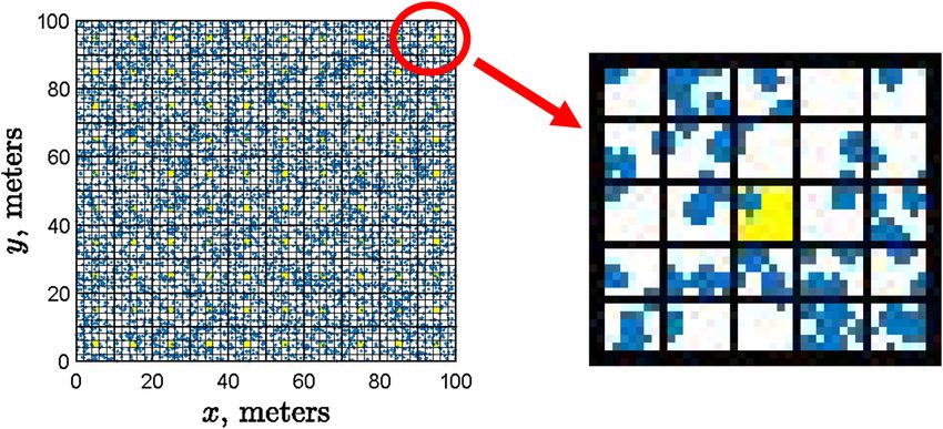
Figure 8. Simulating trap counts. Each bin in the 10 × 10 grid is additionally split into 25 cells, the central cell
(highlighted in yellow) being regarded as the trap’s catchment area. As an example, the right-hand side of the
figure shows the magnified structure of the top-right bin of the study domain. Blue dots show the position of
individual animals. The number of animals in the central cell is used as a proxy for the trap counts.
Evaluating trap counts. In the above, we have shown that our IBM model parameterized using field data
on individual slug movement produces a distinctly heterogeneous, patchy spatial distribution. The degree of
aggregation, both in terms of the Morisita index and Taylor’s aggregation index is higher than it would be due to
purely stochastic reasons. The emerging patchy structure is self-organized in the sense that it emerges not due
to the effect of external factors but due to an inherent property of the system such as the density dependent slug
movement.
The simulated spatial patterns exhibit properties similar to the distribution of slugs in the field, in par-
ticular showing similar values of the aggregation index, which in the field data was found18 to be in the range
1.09 < β < 1.52. There is, however, one difference: while the aggregation of slugs in the field is considered using
trap counts, in our simulations we calculated the total size of the slug population in each bin. Obviously, the
latter is considerably larger than the former, as in reality only a small fraction of the total population is caught
by traps. This explains the difference (almost by an order of magnitude) between numbers shown on the colour
bar in Fig. 1 (a typical example of field data) and the numbers shown on the colour bar in Figs. 2, 3, 4, 5 (simula-
tion results).
In order to resolve this discrepancy, one has to evaluate the trap counts arising from a given population
density distribution in the area around the trap. This is a difficult problem, as it depends on the trap design and
also requires a good understanding of fine details of animal behaviour. Reliable models to calculate trap counts
only exist for the basic case of a completely random Brownian movement (which is not the case that we consider
in this study) and for pitfall-type t raps42–44, i.e. the kind of trap where, once an animal is caught, it is removed
from the field. However, the design of refuge traps used in the related field study18,24 to which we endeavour to
link our results was different. Slugs typically remain in a refuge trap for a variable period of time, but they are
not removed from the field and can leave the trap at any point. Detailed modelling of trap counts arising for this
trap design (e.g. taking into account a variety of slug behavioural responses) requires a separate study and hence
lies beyond the scope of this paper. For the purposes of this paper, we use a different, semi-empirical approach
to evaluate trap counts. Namely, we take into account that the majority of animals caught by a trap over a given
exposition time come from a certain catchment a rea42,43,45, so that the closer is the position of a given animal
to the trap, the larger is the probability for this animal to enter the trap. Note that, for a simpler (Brownian)
movement pattern, the existence and effect of catchment area was earlier shown using rigorous mathematical
arguments43. We assume that, for a sufficiently small catchment area, all animals end up in the trap. In order to
simulate the catchment area, each of the bins in 10 × 10 grid is split to a number of ‘sub-bins’ or cells of a smaller
size (see Fig. 8). We then interpret the total number of animals in the central cell as the trap count.
The spatial distribution of trap counts simulated as described above in the case of 25 cells for each bin in the
10 × 10 grid (equivalent to the grid of traps used in the field) is shown in Fig. 9. Trap counts are calculated after
the initial distribution was allowed to evolve over t = 104 to ensure that a distinct patchy structure emerges. It is
readily seen that the simulated trap counts correspond well to those collected in the field; see Fig. 1 and also18,19
for more examples of field data (in particular, the supplementary material in18 contains data on 167 field visits).
A question arises here regarding whether the aggregation index is sensitive to the characteristics of the proxy
used for local slug abundance, i.e. using the total number of animals in each bin or only the ‘trap count’ in its
central cell. The relation between the mean and the variance of trap counts obtained in the case of 5 × 5 cells is
shown in Fig. 10a. We obtain that, in this case, the aggregation index is approximately 1.09, a slightly lower value
than in the case with no splitting (cf. Fig. 7), albeit clearly larger than one.
In order to check whether the results are sensitive to the size of the catchment area (i.e. to the number of cells
in each bin), we consider an intermediate case of a larger trap catchment area (i.e. splitting to a smaller number
of cells). Figure 10b shows the relation between the mean and the variance of trap counts obtained in the case of
3 × 3 cells. It is readily seen that the results are similar between the two cases and similar to the baseline case with
Scientific Reports | (2022) 12:2274 | https://doi.org/10.1038/s41598-022-05881-w 8
Vol:.(1234567890)www.nature.com/scientificreports/
a 100 8 b 1 8 c 100 8
80 0.8 80
6 6 6
60 0.6 60
4 4 4
40 0.4 40
2 2 2
20 0.2 20
0 0 0 0 0 0
0 20 40 60 80 100 0 0.2 0.4 0.6 0.8 1 0 20 40 60 80 100
Figure 9. The spatial distribution of simulated trap counts (the population size in the central cell, see details
in the text) obtained for N = 104 slugs for different parameters of density dependence: (a) d = 10, R = 1, (b)
d = 1, R = 1 and (c) d = 10, R = 2. Other parameters are as in Fig. 2.
a b
101
100
100
10-1
10-1 100 100 101
Figure 10. The trap count variance plotted against the mean trap count (shown on a log-log scale) calculated
using the central sub-bin in each of 100 large bins for two different number of sub-bins. (a) 5 × 5 cells:
log(v) = 1.091 log(m) + 0.4007, r 2 = 0.9739; (b) 3 × 3 cells: log(v) = 1.151 log(m) − 0.07845, r2 = 0.9636.
Slug movement parameters are the same as in Fig. 7. Before calculating the binned population numbers, the
initial spatial distribution was run for t = 104 time steps to ensure that the emergence of a fully developed
patchy structure.
no splitting (cf. Fig. 7). The aggregation index is consistently larger than one, being approximately between 1.09
and 1.17 for all cases considered, hence indicating a self-organized patchiness (irreducible to purely statistical
reasons) in a good agreement with the field data.
Discussion
For many species, their spatial population distributions are usually distinctly heterogeneous even in a relatively
uniform environment. A number of factors and processes have been suggested as a possible explanation for this
ubiquitous heterogeneity, e.g. see3,46 for a brief review, their applicability depending on the spatial and temporal
scales of the phenomenon. On a multi-generation time scale, formation of spatial patterns is often linked to the
interplay between the population dispersal and the local intra- and interspecific interactions5–7,10. On a shorter,
within-generation time scale, one well known mechanism behind heterogeneous spatial distribution of animal
species is the social behaviour resulting in the formation of mobile animal groups (swarms, flocks, etc.)14,15. A
fingerprint of this mechanism is a high correlation between the individual velocities of the group members16.
In this study, based on the field data collected in our recent 3-year project focused on distribution and move-
ment of the grey field s lug18,19,22–24, we identified a different, new mechanism resulting in a strongly heterogene-
ous ‘patchy’ spatial distribution. This mechanism neither relies on a correlation between individual velocities
nor results in such correlations. Patches of high animal abundance emerge as a result of a specific movement’s
density dependence, i.e. slowing down of individual movement when con-specifics are present nearby, because
of increasing rest times and a more uniform distribution of the turning angle increasing the path’s tortuosity. The
mechanism is investigated in detail using a novel individual-based model that is parameterized using the field
data. It is shown in simulations that the density dependent slug’s movement behaviour leads to formation of a
patchy population distribution. The emerging spatial distributions have the properties closely resembling those
observed in the field, in particular (i) exhibiting similar values of the aggregation index and (ii) showing the
similar rate of temporal changes whereby patches may persist in arable fields for long periods, many throughout
a cropping season.
Scientific Reports | (2022) 12:2274 | https://doi.org/10.1038/s41598-022-05881-w 9
Vol.:(0123456789)www.nature.com/scientificreports/
In a broader context, our findings fall into the widely accepted paradigm stating that ecological systems are
inherently multi-scale and a comprehensive understanding of a phenomenon occurring on a large scale often
requires understanding of processes acting on a much smaller s cale1. Our study provides new evidence of the
linkage between different scales. The field-scale patterns in the slug abundance (with a typical size on the order
of 10 m) are explained by relating them to individual slug movement that occurs on the spatial scale of about
hundred times smaller (on average, tens of c entimeters22).
A question arises about the generality of the new pattern formation mechanism. It immediately evokes
another question as to how typical is the situation where the presence of con-specifics inhibits the individual
movement of each animal, as it is the main prerequisite for our mechanism to act. This is an old problem, origi-
nally considered for humans in a broader context47,48 but more recently extended to animals. It appears that the
animal response is species-specific. While for some species, e.g. see49,50, the presence of con-specifics tends to
increase animal’s movement rate and its performance more generally (without any direct interference or collec-
tive movement), for others, e.g. some avian species51, it is exactly opposite. The existing studies only address a
handful of species; for many species, there is no information at all. However, patches of high animal abundance
are often observed in ground-dwelling invertebrate species, e.g. carabid b eetles52 and fl
atworms53,54. Although
any evidence about their social response to conspecifics is lacking, one can hypothesize that the heterogeneous
distributions observed for those species arise due to the same mechanism.
This paper aims to demonstrate that the small-scale density dependent slug movement can explain the
observed field-scale patterns in the slug distribution, hence relating the field data on two different spatial scales.
Correspondingly, the parameter values of our individual-based model used in simulations were chosen in the
range consistent with field observations. The distributions of step size and turning angle and the probability of
moving are obtained from the field data u nambiguously23; for the parameters where field data do not provide
their value with satisfactory precision, such as R and d, we check the effect of their variation over a reasonable
range. A question can arise here as to what are the properties of the model (e.g. the properties of the emerging
patterns, if any) in the case where all parameters are varied over a much broader range. This might help to shed
light on pattern formation mechanisms more generally. Investigation into this issue would reveal a detailed
structure of the 6-dimensional parameter space of the model. Although beyond the scope of this paper, it should
become a focus of future research.
Another question that our study leaves open is how slugs actually detect the presence of the con-specifics
in their perception range. One option is an olfactory mechanism as it was found to play a role in navigation
of another slug s pecies55, although there is no definitive evidence that it is employed by the grey field slug. An
alternative possibility which has been recorded for several slug s pecies56–58 is following the slime trail, although
this occurs less frequently (8% of trails) in D. reticulatum than in other species. Arguably, slug response to the
presence of con-specifics can be somewhat different depending on the perception details: for instance, slime
trail following may create a correlation in the movement direction (but not necessarily in the movement speed)
while detection over short distances through volatile chemicals is more isotropic and less likely to bring any cor-
relation. More biological evidence is needed to choose between these or other as yet unrecognised mechanisms.
Received: 23 September 2021; Accepted: 3 January 2022
References
1. Levin, S. A. The problem of pattern and scale in ecology. Ecology 73, 1943–1967 (1992).
2. Levin, S. A. Patchiness in marine and terrestrial systems: From individuals to populations. Philos. Trans. R. Soc. B 343, 99–103
(1994).
3. Grünbaum, D. The logic of ecological patchiness. Interface Focus 2, 150–155 (2012).
4. Levin, S. A. & Segel, L. A. Hypothesis for origin of planktonic patchiness. Nature 259, 659 (1976).
5. Hastings, A., Harisson, S. & McCann, K. Unexpected spatial patterns in an insect outbreak match a predator diffusion model. Proc.
R. Soc. Lond. B 264, 1837–1840 (1997).
6. Malchow, H., Petrovskii, S. V. & Venturino, E. Spatiotemporal Patterns in Ecology and Epidemiology: Theory, Models, and Simula-
tions (Chapman & Hall, 2008).
7. Meron, E. Nonlinear Physics of Ecosystems (CRC Press, 2015).
8. Turing, A. M. On the chemical basis of morphogenesis. Philos. Trans. R. Soc. Lond. B 237, 37–72 (1952).
9. Segel, L. A. & Jackson, J. L. Dissipative structure: An explanation and an ecological example. J. Theor. Biol. 37, 545–559 (1972).
10. Holmes, E. E., Lewis, M. A., Banks, J. E. & Veit, R. R. Partial differential equations in ecology: Spatial interactions and population
dynamics. Ecology 75, 17–29 (1994).
11. Getzin, S. et al. Bridging ecology and physics: Australian fairy circles regenerate following model assumptions on ecohydrological
feedbacks. J. Ecol. 109, 399–416 (2021).
12. Klausmeier, C. A. Regular and irregular patterns in semiarid vegetation. Science 284, 1826–1828 (1999).
13. Nathan, R. et al. A movement ecology paradigm for unifying organismal movement research. Proc. Natl. Acad. Sci. USA 105,
19052–19059 (2008).
14. Okubo, A. Dynamical aspects of animal grouping: Swarms, schools, flocks, and herds. Adv. Biophys. 22, 1–94 (1986).
15. Couzin, I. D., Krause, J., Franks, N. R. & Levin, S. A. Effective leadership and decision-making in animal groups on the move.
Nature 433, 513–516 (2005).
16. Couzin, I. D. & Krause, J. Self-organization and collective behavior in vertebrates. In Advances in the Study of Behavior Vol. 32 (eds
Slater, P. J. B. et al.) 1–75 (Academic Press, 2003).
17. Petrovskaya, N. B., Forbes, E., Petrovskii, S. V. & Walters, K. F. A. Towards the development of a more accurate monitoring pro-
cedure for invertebrate populations, in the presence of unknown spatial pattern of population distribution in the field. Insects 9,
29 (2018).
18. Forbes, E. et al. Stability of patches of higher population density within the heterogeneous distribution of the grey field slug (Der-
oceras reticulatum) in arable fields in the UK. Insects 12, 9 (2021).
Scientific Reports | (2022) 12:2274 | https://doi.org/10.1038/s41598-022-05881-w 10
Vol:.(1234567890)www.nature.com/scientificreports/
19. Forbes, E. et al. Sustainable management of slugs in commercial fields: Assessing the potential for targeting control measures. Asp.
Appl. Biol. 134, 89–96 (2017).
20. Glen, D. M., Milsom, N. F. & Wiltshire, C. W. Effects of seed-bed conditions on slug numbers and damage to winter wheat in a
clay soil. Ann. Appl. Biol. 115, 177–190 (1989).
21. Stephenson, J. W. Laboratory observations on the effect of soil compaction on slug damage to winter wheat. Plant Pathol. 24, 9–11
(1975).
22. Forbes, E. et al. Locomotor behaviour promotes stability of the patchy distribution of slugs in arable fields: Tracking the movement
of individual Deroceras reticulatum. Pest Manag. Sci. https://doi.org/10.1002/ps.5895 (2020).
23. Ellis, J. R., Petrovskaya, N. B., Forbes, E., Walters, K. F. A. & Petrovskii, S. V. Patterns of individual movement of the grey field slug
(Deroceras reticulatum) in an arable field. Sci. Rep. 10, 17970 (2020).
24. Forbes, E. Utilising the Patchy Distribution of Slugs to Optimise Targeting of Control: Improved Sustainability Through Precision
Application (PhD Thesis, Harper Adams University, Shropshire, UK) (2019).
25. Taylor, L. R. Aggregation, variance and the mean. Nature 189, 732–735 (1961).
26. Taylor, R. A. J. Taylor’s Power Law: Order and Pattern in Nature (Academic Press/Elsevier, 2019).
27. Turchin, P. Quantitative Analysis of Movement (Sinauer, 1998).
28. Codling, E. A., Plank, M. J. & Benhamou, S. Random walk models in biology. J. R. Soc. Interface 5, 813–834 (2008).
29. Wilson, R. P. et al. Turn costs change the value of animal search paths. Ecol. Lett. 16, 1145–1150 (2013).
30. Edelhoff, H., Signer, J. & Balkenhol, N. Path segmentation for beginners: An overview of current methods for detecting changes
in animal movement patterns. Mov. Ecol. 4, 21 (2016).
31. Jopp, F. & Reuter, H. Dispersal of carabid beetles—Emergence of distribution patterns. Ecol. Model. 186, 389–405 (2005).
32. Piou, C. et al. Simulating cryptic movements of a mangrove crab: Recovery phenomena after small scale fishery. Ecol. Model. 205,
110–122 (2007).
33. Schmitz, O. J. & Booth, G. Modelling food web complexity: The consequences of individual-based, spatially explicit behavioural
ecology on trophic interactions. Evol. Ecol. 11, 379–398 (1997).
34. Ellis, J. R. A Theoretical and Computational Study of Heterogeneous Spatio-temporal Distributions Arising from Density-dependent
Animal Movement with Applications to Slugs in Arable Fields (PhD Thesis, University of Birmingham, 2020).
35. Hui, C., Veldtman, R. & McGeoch, M. A. Measures, perceptions and scaling patterns of aggregated species distributions. Ecography
33, 95–102 (2010).
36. Morisita, M. Measuring of the dispersion of individuals and analysis of the distributional patterns. Mem. Fac. Sci. Kyushu Univ.
Ser. E 3, 65–80 (1959).
37. Kanevski, M. Analysis and Modelling of Spatial Environmental Data (EPFL Press, 2004).
38. Hurlbert, S. Spatial distribution of the montane unicorn. OIKOS 58, 257–271 (1990).
39. Amaral, M. K., Pellico Netto, S., Lingnau, C. & Figueiredo Filho, A. Evaluation of the Morisita index for determination of the
spatial distribution of species in a fragment of araucaria forest. Appl. Ecol. Environ. Res. 13, 361–372 (2015).
40. Hayes, J. J. & Castillo, O. A new approach for interpreting the Morisita index of aggregation through quadrat size. Int. J. Geo-Inf.
6, 296 (2017).
41. Taylor, L. R., Woiwod, I. P. & Perry, J. N. The density-dependence of spatial behaviour and the rarity of randomness. J. Anim. Ecol.
47, 383–406 (1978).
42. Petrovskii, S. V., Bearup, D., Ahmed, D. A. & Blackshaw, R. Estimating insect population density from trap counts. Ecol. Complex.
10, 69–82 (2012).
43. Petrovskii, S. V., Petrovskaya, N. B. & Bearup, D. Multiscale approach to pest insect monitoring: Random walks, pattern formation,
synchronization, and networks. Phys. Life Rev. 11, 467–525 (2014).
44. Bearup, D., Benefer, C. M., Petrovskii, S. V. & Blackshaw, R. Revisiting Brownian motion as a description of animal movement: A
comparison to experimental movement data. Methods Ecol. Evol. 7, 1525–1537 (2016).
45. Thomas, C. F. G., Parkinson, L. & Marshall, E. J. P. Isolating the components of activity-density for the carabid beetle Pterostichus
melanarius in farmland. Oecologia 116, 103–112 (1998).
46. Petrovskii, S. V. Pattern, process, scale, and model’s sensitivity: A comment. Phys. Life Rev. 19, 131–134 (2016).
47. Allport, F. H. Social Psychology (Houghton Mifflin, 1924).
48. Zajonc, R. B. Social facilitation. Science 149, 269–274 (1965).
49. Levine, J. M. & Zentall, T. R. Effect of a conspecific’s presence on deprived rats’ performance: Social facilitation vs distraction/
imitation. Anim. Learn. Behav. 2(2), 119–122 (1974).
50. Sekiguchi, Y. & Hata, T. Effects of the mere presence of conspecifics on the motor performance of rats: Higher speed and lower
accuracy. Behav. Processes 159, 1–8 (2019).
51. Overington, S. E., Cauchard, L., Morand-Ferron, J. & Lefebvre, L. Innovation in groups: Does the proximity of others facilitate or
inhibit performance?. Behaviour 146, 1543–1564 (2009).
52. Alexander, C. J., Holland, J. M., Winder, L., Woolley, C. & Perry, J. N. Performance of sampling strategies in the presence of known
spatial patterns. Ann. Appl. Biol. 146, 361–370 (2005).
53. Murchie, A. K., & Harrison, A. J. Mark-recappture of ‘New Zealand flatworms’ in grassland in Nothern Ireland. In Proceedings of
the Crop Protection in Nothern Britain (Dundee, Scotland, 25-26 February 2004), 63–67.
54. Petrovskaya, N. B., Petrovskii, S. V. & Murchie, A. K. Challenges of ecological monitoring: Estimating population abundance from
sparse trap counts. J. R. Soc. Interface 9, 420–435 (2012).
55. Gelperin, A. Olfactory basis of homing behavior in the giant garden slug, Limax maximus. Proc. Natl. Acad. Sci. USA 71, 966–970
(1974).
56. Cook, A. Homing by the slug Limax pseudoflavus (Evans). Anim. Behav. 27, 545–552 (1979).
57. Cook, A. Field studies of homing in the pulmonate slug Limax pseudoflavus (Evans). J. Moll. Stud. 46, 100–105 (1980).
58. Wareing, D. R. Directional trail following in Deroceras reticulatum (Muller). J. Moll. Stud. 52, 256–258 (1986).
Acknowledgements
This work was partially supported by AHDB through Project no. 21120078 (to E.F. and K.F.A.W.) and by EPSRC
through Project EP/T027371/1 (to S.P.). J.R.E. acknowledges support in the form of a Research Associateship
from the School of Mathematics, University of Birmingham. S.P. was supported by the RUDN University Strategic
Academic Leadership Program.
Author contributions
S.P. and N.P. designed the research; J.E. performed numerical simulations (as part of his PhD Programme under
the supervision of N.P.). Field data was provided by E.F. and K.F.A.W. All authors participated equally in the
discussion and interpretation of results. N.P. prepared the first draft of the manuscript, with contribution from
J.E. and K.F.A.W. S.P. prepared the final version of the manuscript.
Scientific Reports | (2022) 12:2274 | https://doi.org/10.1038/s41598-022-05881-w 11
Vol.:(0123456789)www.nature.com/scientificreports/
Competing interests
The authors declare no competing interests.
Additional information
Supplementary Information The online version contains supplementary material available at https://doi.org/
10.1038/s41598-022-05881-w.
Correspondence and requests for materials should be addressed to N.P.
Reprints and permissions information is available at www.nature.com/reprints.
Publisher’s note Springer Nature remains neutral with regard to jurisdictional claims in published maps and
institutional affiliations.
Open Access This article is licensed under a Creative Commons Attribution 4.0 International
License, which permits use, sharing, adaptation, distribution and reproduction in any medium or
format, as long as you give appropriate credit to the original author(s) and the source, provide a link to the
Creative Commons licence, and indicate if changes were made. The images or other third party material in this
article are included in the article’s Creative Commons licence, unless indicated otherwise in a credit line to the
material. If material is not included in the article’s Creative Commons licence and your intended use is not
permitted by statutory regulation or exceeds the permitted use, you will need to obtain permission directly from
the copyright holder. To view a copy of this licence, visit http://creativecommons.org/licenses/by/4.0/.
© The Author(s) 2022
Scientific Reports | (2022) 12:2274 | https://doi.org/10.1038/s41598-022-05881-w 12
Vol:.(1234567890)You can also read