A mathematical model of reward-mediated learning in drug addiction
←
→
Page content transcription
If your browser does not render page correctly, please read the page content below
Modeling the neurobiology of drug addiction

                                            A mathematical model of reward-mediated learning in drug addiction
                                                      Tom Chou1 and Maria R. D’Orsogna2
                                                      1) Department   of Computational Medicine, UCLA, Los Angeles, CA 90095-1766, USAa)
                                                      2) Department   of Mathematics, California State University at Northridge, Los Angeles, CA 91130-8313,
                                                      USA b)
                                                      (*Electronic mail: dorsogna@csun.edu)
                                                      (Dated: 24 May 2022)
                                                      Substances of abuse are known to activate and disrupt neuronal circuits in the brain reward system. We propose a
                                                      simple and easily interpretable dynamical systems model to describe the neurobiology of drug addiction that incorpo-
                                                      rates the psychiatric concepts of reward prediction error (RPE), drug-induced incentive salience (IST), and opponent
arXiv:2205.10704v1 [q-bio.NC] 22 May 2022

                                                      process theory (OPT). Drug-induced dopamine releases activate a biphasic reward response with pleasurable, positive
                                                      “a-processes” (euphoria, rush) followed by unpleasant, negative “b-processes” (cravings, withdrawal). Neuroadaptive
                                                      processes triggered by successive intakes enhance the negative component of the reward response, which the user com-
                                                      pensates for by increasing drug dose and/or intake frequency. This positive feedback between physiological changes
                                                      and drug self-administration leads to habituation, tolerance and eventually to full addiction. Our model gives rise to
                                                      qualitatively different pathways to addiction that can represent a diverse set of user profiles (genetics, age) and drug
                                                      potencies. We find that users who have, or neuroadaptively develop, a strong b-process response to drug consumption
                                                      are most at risk for addiction. Finally, we include possible mechanisms to mitigate withdrawal symptoms, such as
                                                      through the use of methadone or other auxiliary drugs used in detoxification.

                                            Drug abuse has been dramatically increasing worldwide                    addiction. Finally, our model can be used to explore detox-
                                            over the last twenty years. Despite attempts to implement                ification strategies.
                                            effective prevention programs, treatment options, and leg-
                                            islation, drug poisoning remains a leading cause of injury-
                                            related death in the United States, with a record 100,000
                                            fatal overdoses recorded in 2020. Understanding how an                   I.   INTRODUCTION
                                            addiction to illicit substances develops is of crucial impor-
                                            tance in trying to develop clinical, pharmaceutical, or be-
                                            havioral interventions. The neurobiological basis of drug                   Despite decades of medical, political, and legal efforts, sub-
                                            addiction is centered on disruptions to the dopamine sys-                stance abuse remains a major issue worldwide. The annual
                                            tem in the brain reward pathway of users, which lead to                  number of overdose deaths in the United States has risen from
                                            neuroadaptive changes and the need for larger or more                    about 20,000 in 2000 to over 70,000 in 20191, resulting in the
                                            frequent intakes to avoid withdrawal symptoms. Despite                   highest drug mortality rate in the world at an economic cost
                                            the many qualitative descriptions of the pathway to addi-                of at least $740 billion USD per year2 .
                                            tion, a concise mathematical representation of the process                  Our understanding of addiction, why and how it emerges, is
                                            is still lacking. We propose a unified, easily interpretable             still incomplete although several mechanisms of action have
                                            dynamical systems model that includes the concepts of                    been identified3,4 and modeled5,6 . Addictive substances hi-
                                            reward prediction error (RPE), drug-induced incentive                    jack the mesocorticolimbic pathways which govern our re-
                                            salience (IST) and opponent process theory (OPT). Specif-                sponse to primary rewards such as food, drink, and sex. Un-
                                            ically, we introduce a time-dependent reward function                    der normal conditions, primary rewards increase levels of
                                            associated with each drug intake. Physiological param-                   dopamine, the main neurotransmitter in the brain reward sys-
                                            eters evolve through neuroadaptation, consistently with                  tem. Dopamine-strengthened neuronal connections encode
                                            OPT, while user-regulated drug intake is dependent on                    information on the reward and its utility7,8 , while its release in
                                            the most recent reward prediction, consistent with RPE.                  the mesocorticolimbic pathways regulates incentive salience,
                                            Our model yields different distinct stages of the addiction              the want and seeking of rewards 9,10 . To optimize future re-
                                            process that are cycled through via a dynamical recursion.               sponses, dopaminergic neurons respond differently to rewards
                                            Individual-specific parameters may be tuned to represent                 that deviate from expectations11–13 . The reward prediction er-
                                            different drug potencies, age, or genetic predispositions.               ror (RPE) quantifies the discrepancy between a reward and its
                                            Rich features emerge, such as monotonically convergent                   prediction and plays a major role in learning: neural activity
                                            or damped oscillatory ("yo-yo") progression towards full                 increases if the reward is greater than expected (positive RPE)
                                                                                                                     and decreases otherwise (negative RPE)14–16 . The RPE em-
                                                                                                                     bodies reinforcement learning, a key concept in psychology
                                                                                                                     that has been modeled and applied to many contexts, includ-
                                            a)
                                              Also at Department of Mathematics, UCLA, Los Angeles, CA 90095-1555,   ing drug addiction5.
                                            USA                                                                         The effects of addictive drugs on the brain are similar to that
                                            b) Also at Department of Computational Medicine, UCLA, Los Angeles, CA
                                                                                                                     of primary rewards; drugs however amplify desires in abnor-
                                            90095-1766, USA                                                          mal ways. Viewed as rewards, cocaine, amphetamines, and
Modeling the neurobiology of drug addiction                                                                                             2

morphine act faster and increase dopamine levels two to ten         drug intake
times more than food or sex17–19 , exaggerating the brain’s
response to any drug-related cue. The operational mecha-
nisms of each drug type may be different, for example co-
caine blocks the reuptake of dopamine, whereas heroin binds
to mu-opioid receptors which directly stimulate the release of
dopamine. Other molecular targets of drugs of abuse include
the neurotransmitters endorphin and enkephalin (particularly        FIG. 1. Schematic of a- and b-processes. Drug use activates the
in the case of prescription opioids) and norepinephrine and         dopaminergic neurons which in turn activate the hedonic hotspots in
glutamate20,21 . Signaling between different neurotransmitter       the nucleus accumbens that mediate the pleasurable “a-processes”
types frequently leads to secondary effects. Whether directly       wa , leading to euphoria and bliss. Unpleasurable “b-processes” wb
or indirectly activated the most common feature of drug intake      may follow, accompanied by cravings and withdrawal symptoms.
is a dramatic increase in dopamine signaling in the nucleus ac-     The relative magnitude of the two wa,b experiences may vary among
                                                                    individuals and may depend on the stage of addiction. Dopamine-
cumbens (NAc)22 , which is the process we will focus on in our
                                                                    induced activity is modeled as D(t) = ∆e−δ t where ∆ is a proxy
modeling.                                                           for drug dosing and δ its typical degradation rate. The overall a-
   Incentive sensitization theory (IST) formalizes the concepts     process is activated by D(t) via the prefactor Γa , whereas the over-
illustrated above23. Another relevant psychological concept         all b-process is activated by the a-process via the prefactor Γb . The
is opponent process theory (OPT) whereby every emotional            activity of the a- and b-processes decay with rates α and β , respec-
experience, pleasant or unpleasant, is followed by a counter-       tively.
acting response to restore homeostasis. Within OPT, the con-
sumption of drugs induces an “a-process,” marked by eupho-
ria, rush, and pleasure, later compensated by a “b-process”         cally defined as the state in which the overall reward is nega-
marked by withdrawal symptoms, and craving24,25 . For be-           tive and the reward prediction error is below a given threshold.
ginning users, the pleasant a-process is more intense and lasts     These formulations allow us to predict the unfolding of the ad-
longer than the unpleasant b-process. Continued use leads to        diction process depending on the specific physiology and neu-
neuroadaptation, with the b-process appearing earlier and last-     roadaptive profile of the user. Specifically, we find that, given
ing longer. Tolerance and dependence set in26,27 as drug con-       the same drug, users who are more sensitive to neuroadaptive
sumption becomes predominantly unpleasant28. Examples               changes in the b-process (or who have an initially elevated b-
of drug-dependent neuroadaptation include the reduction of          process response) are the ones whose progression to addiction
postsynaptic D2 dopamine receptors29, neuronal axotomy30,           is faster than those who are less reactive. These more resilient
decreased dopamine neuron firing31 , increases in the number        users may also display reward prediction errors that oscillate
of AMPA receptors32, and activation of D1-like receptors33.         in value with each drug intake before permanently crossing
Central among the brain tissues responding to drug use is the       the threshold to addiction (“yo-yo” dynamics).
ventral tegmental area (VTA) whose dopaminergic neurons
project to the nucleus accumbens (NAc) shell and to the ven-
tral pallidum (VP), two of the brain’s pleasure centers asso-       MATHEMATICAL MODEL
ciated with the a-process. The neurobiological source of the
b-process has been identified with the subsequent activation        Dopamine release
of several stress circuits controlled by the extended amygdala
and the hypothalamus, disrupting the release of stress related         We begin by describing the time-dependent activity D(t)
hormones or peptides such as CRH, norepinephrine, dynor-            (e.g., firing rate) of dopaminergic neurons in the reward sys-
phin, hypocretin, leading to aversive feelings24,34–36 .            tem in response to the dopamine release that follows a single,
   How drugs impact the brain reward system has been                initial drug intake. Other rewards such as food, sex, etc. also
mathematically studied using dynamical systems 5,37–41 , real-      stimulate dopamine release, however, it is known that drug-
time neural networks 42,43 , temporal-difference reinforcement      induced dopamine release is an order of magnitude larger than
learning 44 , and model-free learning models 45 . While these       what stimulated by “natural” rewards17. Experimental mea-
models explain certain observed features of the addiction pro-      surements show a rapid rise in activity within a few minutes
cess, a simpler, yet explicit quantitative framework that unifies   of intravenous drug administration46,47 , followed by an expo-
concepts from RPE, IST, OPT, and allostasis is still lacking.       nential decay over one to five hours17. We propose
Here, we construct and analyze a proof-of-principle mathe-
matical model of the onset of drug addiction, resolved at the                                 D(t) = ∆e−δ t ,                         (1)
individual drug intake time scale. Neuroadaptation is repre-
sented by changes in physiological parameters consistent with       where ∆ is the magnitude of the dopamine response and 1/δ
RPE and OPT, informing changes to user behavior. These              is the effective dopamine residence time which includes the
changes induce further neuroadaptation, creating a feedback         clearance time of dopamine-stimulating drugs; typically δ ∼
loop that may lead to full addiction. We introduce measures to      0.2 − 1 hr−1. For simplicity we measure time in units of δ ,
quantify the overall reward resulting from a single drug intake     rescale t ′ → δ t, drop the prime notation, and set D(t) = ∆e−t .
and for the reward prediction error; addiction is mathemati-        Since dopamine release is triggered by drug intake we hence-
Modeling the neurobiology of drug addiction 3
(a) (b)
2
I 1.5 1.3
1 1
II
III 0.5 0.825
0 0.7
0 0.5 1 1.5 2
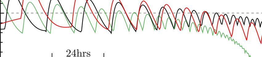
FIG. 2. (a) Three examples of time-dependent response w(t|θ ) associated with a single, isolated dopamine hit. We fix θ = {∆ = 1, α =
0.5, Γa = 1, β , Γb = 0.8} and plot Eq. 4 for three different values of β showing a response that is always positive (I: β = 1.5, orange), a
response that can become negative (II: β = 0.9, green), and one with a negative total reward (III: β = 0.45, blue). (b) Density plot representing
the values of the time t ∗ associated with the solution to the transcendental equation w(t ∗ |θ ) = 0 as a function of β and Γb for α = 0.5. The
white parameter region does not admit a finite solution to t ∗ (w(t|θ ) is always positive).
forth use ∆ as a proxy for drug dosage. Although more com- The wa,b (t) processes generate the brain reward system’s
plex pharmacokinetic models have been developed to con- perception of the drug. While further complex processing
nect drug dose to dopamine activity48 , the time dependence and filtering of wa,b (t) may be at play, we assume they
of dopamine activity qualitatively resembles a decaying expo- are summed to yield the dynamic, time-dependent response
nential except at very short times. w(t|θ ) = wa (t)+ wb (t) where θ = {∆, α , Γa , β , Γb } are the pa-
rameters associated with the reward perception process. Upon
solving Eqs. 2 and 3, we find the dynamic response w(t|θ ) fol-
Single-dose drug-induced a- and b-processes lowing a single, isolated dopamine release and/or drug intake
According to OPT and as described above, drug-induced
Γa ∆ Γb Γb
dopamine activity D(t) induces a pleasurable a-process, wa (t), w(t|θ ) = 1− e−t − 1 − e− α t
which in turn activates an unpleasant b-process, wb (t) (see α −1 β −1 β −α
b
Fig. 1). We propose a deterministic model for wa,b (t) that in- Γb
Γ −β t
corporates simple integrate-and-fire dynamics − − e . (4)
β −α β −1
The time-integrated net response
dwa (t)
= −α wa (t) + Γa D(t) (2)
dt
Γa ∆ Γb
Z ∞
dwb (t)
= −β wb (t) − Γb wa (t), (3) W (θ ) = w(t|θ )dt = 1− , (5)
dt 0 α β
where Γa and Γb represent the coupling of D(t) to wa (t), and associated with a single, isolated dopamine release and/or
of wa (t) to wb (t), respectively. The intrinsic decay rates of drug intake can be interpreted as a memory of the experience,
the a- and b-processes are denoted α and β . The effects of and can be used as a benchmark for future decision-making.
intermittent natural rewards that induce dopamine release can Note that the amplitude factor Γa in Eqs. 4 and 5 adjusts the
be incorporated by including an extra source to wa (t) in the “hedonic” scale of w(t|θ ) and W (θ ).
form of a periodic or a randomly fluctuating term. These In Figure 2(a), we plot w(t|θ ) for ∆ = 1, α = 0.5, Γa =
non-drug terms would be much smaller in magnitude than the 1, Γb = 0.8, and β = 1.5 (orange curve I), β = 0.9 (green
drug source D(t), since drug induced stimuli are much larger curve II), and β = 0.45 (blue curve III). These representa-
than non-drug ones17 . The periodic part may represent, say, tive response curves w(t|θ ) are: I, always positive; II, turning
eating at regular intervals, whereas the fluctuating part might negative with positive integral W (θ ) > 0; and III, turning neg-
describe all other non-drug, pleasurable experiences that oc- ative with negative integral W (θ ) < 0. Type I responses are
cur at random times. Thus, a stochastic model might yield typical of healthy, naïve users who for the most part experi-
a more complete description of the brain reward system and ence only the pleasurable a-process. For smaller β , larger Γb ,
its many inputs but we shall limit this study to the determin- and/or larger α (Γb < β < Γb + α ), w(t|θ ) exhibits a type II
istic response from well-defined drug intakes as presented in response which is negative at late times but yields a positive
Eqs. 2-3. net response W (θ ) > 0. For even smaller β and/or larger Γb ,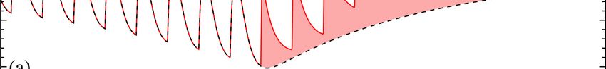
Modeling the neurobiology of drug addiction                                                                                                   4

      0.6
                                                                        where θi = {∆i , αi , Γai , βi , Γbi } are the parameters of the sys-
                                                                        tem following intake i. The doses ∆i and intake times Ti are
      0.4
                                                                        primarily user-controlled. We assume the other parameters
                                                                        {αi , Γai , βi , Γbi } evolve in a step-wise fashion due to dopamine-
      0.2
                               +               - +                      induced neuroadaptive changes, such as long term potentia-
                                                                        tion or other long-lasting physiological, tissue-level, or bio-
       0
                                                                        chemical processes. The total net response after the last dose
                                         -                  -           at time Tk can be defined as an integral over w(t|{θi≤k }) start-
     -0.2
                                                                        ing from Tk until the current time t. Thus, the net response
     -0.4                                                               associated with dose k is
                                                                                                             Z t
                                                                                   Wk (t|{θi≤k , Ti≤k }) =         w(t ′ |{θi≤k })dt ′ ,     (7)
                                                                                                              Tk
FIG. 3. Time-dependent response w(t) resulting from multiple drug
intakes at times T1 = 0 (not shown), T2 , T3 , and T4 . Each dopamine   where Tk < t < Tk+1 and Tk+1 is the time of the next dose, if it
release elicits an a- and b-process response which can be concate-      occurs. Using Eqs. 4 and 7, we find
nated (Eq. 6). The net reward Wk associated with dose k is defined
as the integral of w(t|{θi≤k }) from time Tk to Tk+1 and may depend
on θi≤k since the a- and b-processes triggered by previous drug in-                                 k
takes may not have fully dissipated. For small βi , b-processes re-        Wk (t|{θi≤k , Ti≤k }) = ∑ Ci (e−(Tk −Ti ) − e−(t−Ti ) ) +
lax slowly making the response to appear to reach a lower home-                                    i=1
ostatic value. The small β regime resembles the allostatic effect                                   k
on time scales . 1/β . In this limit, repeated drug doses succes-                                  ∑ Ciα (e−αi (Tk −Ti ) − e−αi(t−Ti ) ) +
sively drive the reward response negative pushing the user to ex-                                  i=1
perience increasingly intense withdrawal symptoms. In these plots,                                  k
∆ = 1, α = 0.2, Γa = 1, Γb = 0.2 and β1 = 0.3, β2 = 0.2, β3 = 0.1,                                       β
and β4 = 0.1 for intakes at 0, T, 2T and 3T , respectively. The RPE
                                                                                                   ∑ Ci (e−βi(Tk −Ti ) − e−βi(t−Ti ) ),      (8)
                                                                                                   i=1
is defined by the difference between two consecutive time-integrated
responses Wk −Wk−1 .                                                    where
                                                                                           Γai ∆i        Γbi

                                                                                      Ci ≡          1−          ,
the response is type III: the negative b-process overtakes the a-                          αi − 1      βi − 1
process and the overall experience is negative with W (θ ) < 0.                            Γai ∆i 1

                                                                                                        Γbi

                                                                                       α
Type II and type III responses are typical of moderate and ad-                       Ci ≡                     −1 ,                           (9)
dicted users, respectively. Figure 2(b) shows the density plot                             αi − 1 αi βi − αi
of the time t ∗ when the dynamic response w(t ∗ |θ ) = 0, as a                             Γai ∆i 1    Γbi        Γbi

                                                                                       β
                                                                                     Ci ≡                    −          .
function of β and Γb at α = 0.5. For β ≥ Γb + α there are no                               αi − 1 βi βi − 1 βi − αi
finite solutions t ∗ to w(t ∗ |θ ) = 0; in this regime the dynamic
response is always positive as represented by the type I curve          If drug intakes are well-separated (Ti+1 − Ti → ∞) with no
in Figure 2(a). For β < Γb + α , t ∗ is positive and finite and         residual effects from previous doses, the net response between
decreases as β decreases or Γb increases, indicating a stronger         Tk and Tk+1 is Wk (Tk+1 |{θi≤k , Ti≤k }) → Γak ∆k (1 − Γbk /βk )/αk ,
overall b-process. Examples are the type II and type III curves         the result given in Eq. 5.
in Figure 2(a).
   What we have described so far is a simple single-dose pic-
ture of the reward response. In the next section we build on            Reward prediction error (RPE) and behavioral changes
it to describe addiction as a progression of multiple drug in-
takes that induce neuroadaptive changes to the physiological               To construct the total time-dependent response for multi-
parameters, β and Γb , and behavioral changes to the user that          ple drug intakes w(t|{θi≤k }) in Eq. 6, we must describe the
shift the net response from type I to type III.                         evolution of the user-controlled variables {∆i , Ti } and of the
                                                                        neuroadaptive parameters {αi , Γai , βi , Γbi } as a function of the
                                                                        number of intakes i. In this section, we provide a mathemat-
Successive drug intakes                                                 ical description of the RPE, the difference between the ex-
                                                                        pected and received rewards associated to each drug intake.
   We now consider successive drug intakes i taken at times             The RPE is a key component of learning and decision-making;
Ti with the first dose taken at T1 = 0 and the most recent one          here it will be assumed to regulate the specific decision of the
at Tk . For finite Tk , the total time-dependent response is a          user to change (or not) the next drug dose ∆k+1 of intake k + 1.
superposition of the time-shifted responses in Eq. 4                       The expected response of a drug intake depends on the
                    k
                                                                        user’s prior history, experiences, and cues of upcoming re-
  w(t|{θi≤k }) = ∑ w(t − Ti |θi ), T1 ≡ 0, Tk < t < Tk+1 , (6)          wards. The expectation may be different from the actual, ob-
                   i=1                                                  tained response leading to an error, the RPE. For simplicity,
Modeling the neurobiology of drug addiction 5
we represent the RPEk following intake k, and just before in- yielding an apparent “allostatic” state49 . In the above recur-
take k + 1, as the difference between the most recent net re- sion Eq. 11, the drug doses ∆i may be assumed fixed or may
sponse Wk and the prior one Wk−1 evolve according to models that involve the RPE.
We now incorporate the ingredients described above into a
RPEk ≡ Wk (Tk+1 |{θi≤k , Ti≤k }) dynamical model that generates trajectories to addiction. In
−γk−1Wk−1 (Tk |{θi≤k−1 , Ti≤k−1 }) − Ck+1, (10) this model, the neuroadaptative evolution of the physiological
parameters induces changes to the reward responses, which in
weighted by a factor γk−1 < 1 that discounts the previous turn modify the RPE and lead to user behavioral changes such
net response Wk−1 and that may incorporate memory effects. as increases in drug dose or intake frequency to boost the plea-
RPEs that rely on responses associated with drug doses fur- surable a-process. Despite these user-controlled changes, the
ther in the past can also be used to reflect longer memory of evolving neurophysiological parameters may eventually lead
the reward37. The term Ck+1 is a history-independent cue as- to negative net responses and RPEs. We thus define addiction
sociated with the upcoming k + 1th intake. Examples of cues as a state marked by persistently negative RPEi < 0 and neg-
include seeing or smelling the drug, or preparing for its con- ative net responses Wi < 0 that arise for intakes at or greater
sumption. Without loss of generality, we assume Ck = 0 by than a critical number i ≥ k∗ .
shifting the baseline value of the RPE. An example of a nega-
tive RPE is shown in Fig. 3, where RPE3 < 0 indicating unmet
expectations from intake 3. As defined in Eq. 10, a positive Evolution of intake doses
RPEk arises if Wk > γk−1Wk−1 , raising expectations for future
intakes. This increased expectation may represent habitua- We first consider the case where the intake times Ti =
tion, whereby continued use generates a desire for greater net (i − 1)T are perfectly periodic with interval T and study the
responses. The value of RPEk will be used in the next section evolution of the most recent dose ∆k to the next one ∆k+1 .
to determine if a behavioral change – another drug intake at Although more intense dopamine activity may be stimulated
time Tk+1 and/or a change in dose ∆k+1 – is elicited. by a larger ∆k+1 (according to Eq. 4 for well spaced intakes),
the resulting net response Wk+1 may not necessarily be larger
than Wk since Wk+1 depends not only on dose, but also on
Neuroadaptation and parameter changes the neuroadaptive parameters {αk+1 , Γak+1 , βk+1 , Γbk+1 } over
which the user has no direct control. Thus, scenarios may
arise in which although the drug dose increases, the RPE re-
In addition to {∆, Ti }, the time-dependent response
mains negative and user expectations are not met. We assume
w(t|{θi≤k }) also depends on the physiological parameters
that if the RPE > 0 the user will not alter drug dose; how-
{αi , Γai , βi , Γbi }. Changes in these quantities can be driven by
ever, if RPE < 0 the user will increase it. To concretely model
neuroadaptive processes following each drug intake and can
this behavior and allow variable ∆k , we augment the recursion
depend on the specific characteristics (age, gender, constitu-
relations 11 as follows
tion, genetic makeup) of each user. These neuroadaptive pro-
cesses are complex and difficult to model, so we simplify mat- 1 x ≤ Rc
x
ters by assuming that {αi , Γai , βi , Γbi } change only in response ∆k+1 = ∆k + σ H(RPEk ), H(x) = R c Rc < x < 0
to each drug-induced dopamine release ∆i at Ti . To be con- 0 x ≥ 0,
sistent with OPT and observations, neuroadaptative changes (12)
should increase the effects of the negative b-process relative to where σ is the maximal dose-change and H(x) dictates how
those of the positive a-process as addiction progresses. This doses increase as a function of RPEk . We choose the simple
can be achieved through a decrease in βi and/or an increase form in Eq. 12 representing a graded switching function with
in Γbi . In principle, changes in αi arising from tolerance (that threshold Rc /2. We use the representation of RPEk given in
shortens the “high” and affects the relative strengths of the a- Eq. 10 in which for simplicity we set γk−1 = 1 and Ck+1 = 0.
and b-processes) can also be modeled, but since changes to Finally, note that the argument of H in Eq. 12, RPEk , de-
Γai ∆i /(αi − 1) only rescale w(t), we fix αi = α and Γai = Γa to pends on the drug intake period T and the dose ∆k through
constant values. Thus, we let ∆i drive neuroadaptive changes Wk (Tk+1 |{θi≤k , Ti≤k }), which makes the evolution Eq. 12 non-
in βi+1 and Γbi+1 according to the simplest rule consistent with linear.
OPT: In our model, changes to the neuroadaptive parameters
βi+1 , Γbi+1 at intake i + 1 carry a linear dependence on the
βi+1 = βi (1 − B∆i+1), Γbi+1 = Γbi (1 + G∆i+1). (11) dosage ∆i+1 , according to Eqs. 11. We adopted this choice
for simplicity; however more complex forms for the evolution
Here, B and G are parameter-change sensitivities that may de- of βi+1 , Γbi+1 and ∆i+1 can be used to study a wider range of
pend on i, βi , Γbi , and ∆i , but that we assume to be constant, scenarios.
with the caveat that B is small enough that for all values of i, Specifically, the parameters coefficients B, G in Eqs. 11
B∆i < 1. Equation 11 implies that βi and Γbi are represented could be modeled to be functions of intake number or time on
by piecewise constant values that change after each drug in- drugs, through forms that depend on the genetics of age of the
take. Note that after a sufficient number of intakes βi becomes user. Such refinements may be important especially if one is
very small and the negative response persists for a long time, interested in the long-term dynamics of drug consumption, orModeling the neurobiology of drug addiction 6
1
0.5
0
-0.5
T T T T T T T
0.75 4 0.5
(b) (c) (d)
3
0.5
2
0
1
0.25
0
0 -1 -0.5
1 5 10 15 20 25 30 1 5 10 15 20 25 30 1 5 10 15 20 25 30
FIG. 4. (a) The time-dependent response resulting from multiple drug intakes with varying ∆k for three scenarios. In Case 1 (solid black
curve), we set B = 0.05, G = 0 while in Case 2 (dashed green curve), B = 0, G = 0.05. Finally, in Case 3 (solid red curve), B = G = 0.05.
The interval between two consecutive intakes in these examples is T = Tk+1 − Tk = 6. The effects of neuroadaptation when both βk and Γbk
evolve are synergistic as Case 3 leads to addiction after significantly fewer intakes. (b) Evolution of the parameters βk (open circles, solid
curves) and Γbk (filled circles, dashed curves) for Cases 1, 2, and 3. (c) Evolution of the integrated response and intake doses ∆k (blue triangles,
Eq. 12) associated with intake k for each of the three cases. The evolution of ∆k is similar for Cases 1 and 2, while ∆k for Case 3 rises faster
and might describe a highly addictive drug that results in addiction after a smaller number of doses. The integrated responses Wk become
negative at about intake k ≈ 27, 26, and 16 for Cases 1, 2, and 3, respectively. (d) The RPEk as a function of the intake k exhibit oscillations
with increasing then decreasing amplitude before monotonically decreasing well below zero at intakes k ≈ 20, 18, and 10 for Cases 1,2, and
3, respectively. In all cases, the user experiences a “yo-yo” progression to addiction. Since in all cases, Wk becomes negative after the RPE,
addiction occurs when Wk < 0 at intakes k∗ ≈ 27, 26, and 16, respectively.
in comparing responses among different user types. For exam- We let the second dose ∆2 = 1 and generate {β2 , Γb2 } from
ple, it is well known that drugs of abuse can significantly im- Eq. 11 and W2 (T3 |{θi≤2 , Ti≤2 }) from Eq. 7, yielding RPE2 =
pact the still-maturing, and thus vulnerable, adolescent brain W2 (T3 |{θi≤2 , Ti≤2 }) − W1 (T2 |{θ1 , T1 }). The next dose ∆3 is
and cause severe, long-term damage50. Eqs. 11 can also be then determined through Eq. 12, and so on. To illustrate
modified to include saturation, or recovery of the baseline val- responses to multiple fixed-period intakes, we must specify
ues of βi+1 , Γbi+1 if the user stops using drugs. Other nonlin- the dimensionless time T between drug intakes relative to the
earities may be introduced to represent distinct neuroadaptive drug-induced dopamine mean residence times. In Fig. 4, we
regimes. These could be stages of more (or less) impactful assume the inter-intake period T to be six times the effective
changes once a given threshold of, say, drug dose, cumulative dopamine residence time 1/δ . Thus, if δ ≈ 0.25/hr, daily drug
drug dose, or reward value is reached51. These choices may dosing (once every 24hrs) corresponds to T = 6.
lead to non-trivial dynamics involving β , Γb , ∆ as well as the Figure 4(a) shows the total time-dependent response
RPE, and possibly lead to chaotic behaviors52, as proposed in w(t|{θi }) under three sets of parameters, B = 0.05, G = 0
the context of alcohol addiction53–55 . (Case 1, solid black curve), B = 0, G = 0.05 (Case 2, dashed
green curve), and B = G = 0.05 (Case 3, solid red curve). We
see that under neuroadaptation of both parameters β and Γb
RESULTS (Case 3), the transition to addiction occurs much faster (red
curve), with a shorter plateau in Wk and a quicker drop in
We now study the effects of multiple intakes utilizing the RPEk . In general, a larger Γb relative to Γa depresses the time-
full model given by Eqs. 7–9 and Eqs. 10–12. We set αi = dependent dynamical response w(t|{θi }) and the net response
0.3, Γai = 1, Rc = −0.05, σ = 0.1, initialize the system with W . Larger α and β lead to more transient responses that dis-
{β1 , Γb1 , ∆1 , RPE1 } = {0.5, 0.1, 1, 0}. Upon specifying B, G play less overlap between intakes provided T is fixed. Smaller
we can find the first net response W1 (T2 |{θ1 , T1 }) per Eq. 7. β leads to longer lasting b-processes that overlap across suc-Modeling the neurobiology of drug addiction 7
3
2
1
0
-1
-2
T T T T T T T T
0.5 16 3
(b) (c) (d)
0.4 12 2
0.3 8
1
0.2 4
0
0.1 0
0 -4 -1
1 5 10 15 20 25 30 35 1 5 10 15 20 25 30 35 1 5 10 15 20 25 30 35
FIG. 5. (a) The time-dependent response resulting from multiple drug intakes at times Ti = (i − 1)6 with user-adjusted ∆i for three additional
scenarios corresponding to different durations 1/α of the a-process. In Case 4 (black solid curve), we keep β1 = 0.5, Γa = 1, Γb1 = 0.1, σ = B =
0.05, G = 0 but assume a long-lasting a-process by setting α = 0.05. In Cases 5 (green dashed curve) and 6 (solid red curve) we use α = 0.2
and α = 0.7, respectively. The corresponding βk and Γbk for these cases are nearly indistinguishable, as shown in (b). The corresponding doses
(blue triangles) shown in (c) are also indistinguishable. The integrated responses Wk for these three cases reach long-lived plateaus of different
amplitudes. The associated RPEs are also qualitatively different, as shown in (d). In all cases, the RPEs hover around small values for many
intakes. Note while longer-lasting a-processes generate higher values of Wk , the corresponding RPEs decrease faster. Addiction in these three
cases occur at k∗ ≈ 33, 30, and 31 when Wk < 0 since RPEk < 0 occurs at k ≈ 11, 5 and 2.
cessive intakes. exhibits a smaller amplitude. These results indicate that the
In Fig. 5 we explore the effects of varying the duration sensitivity of the responses, Wk , and RPEk to changes in α are
nonlinear and involve a subtle interplay between the overlap
of the a-process by setting β1 = 0.5, σ = 0.05, Γa = 1, Γb1 =
0.1, B = 0.05, G = 0 and changing α . In Cases 4, (solid black of the a- and b-processes the amplitude Γb of the b-process,
and the definition of the RPE.
curves), 5 (dashed green curves), and 6 (solid red curves)
we set α = 0.05, 0.2, 0.7 to represent long-lasting, interme- The cases described above are illustrative of how differ-
diate, and short-lived a-processes, respectively. As shown in ent user-specific parameters (B, G, σ , α ), and initial conditions
Fig. 5(a), a smaller α results in more overlap of positive re- (β1 , Γb1 ) yield qualitatively different paths to addiction. Cases
sponses wa and as a result, more positive overall response 1,2, and 3 reveal the effects of higher neuroadaptive sensitivity
w(t|θi≤k ). Different values of α do not seem to apprecia- (Case 3, B = G = 0.05) whereby the onset of addiction is dra-
bly change the number of intakes at which w(t|θi≤k ) becomes matically faster. Cases 4,5, and 6 compare scenarios in which
negative. The evolution of βk and ∆k are nearly indistinguish- the trajectories of the neuroadaptive parameter βk and intake
able for all three cases as shown in Fig. 5(b) and (c). dose ∆k do not substantially differ but can nonetheless lead
to qualitative differences in the magnitudes of the integrated
It is worth noting that, as shown in Fig. 5(c), the net re- response Wk , the drop-off point of the RPEk , and the intake
sponses Wk in Cases 4,5,6 reach long-lasting plateaus before at which addiction occurs. The yo-yo behavior of RPEk is
starting to decrease, between intakes k = 30 and k = 35. The typically seen for users who are allowed to adjust their doses
corresponding RPEs shown in Fig. 5(d) fluctuate around zero through Eq. 12.
in all cases until relatively large intake numbers k are reached,
indicating “high-functioning” users. Eventually however the
RPEs decrease and become negative as well. However, the
quickest decent of the RPEk towards negative values is ob- Evolution of intake timing
served for the longest lived a-process, Case 4 for α = 0.05,
whereas the most stable RPEk arises for the shorted lived a- We now consider the case where drug doses are equal for all
processes, Case 6 for α = 0.7, although the associated Wk intakes ∆i ≡ ∆ = 1, but the user-controlled intake times Ti doModeling the neurobiology of drug addiction 8
0.5 10
(a) (b)
8
0 6
4
-0.5 2
0
30 40 50 60 70 80 0 10 20 30 40
FIG. 6. (a) Time-dependent response curves resulting from multiple drug intakes with varying Tk are generated using α = 0.5, Γa = 1, B = G =
0.01 and β1 = Γb1 = 0.5. Case 1T (solid black curve) assumes γk = γ = 0 and no memory before the last intake, while Cases 2T (solid black
curve) and 3T (dashed red curve) assume intermediate and strong memory, γk = γ = 0.5 and γk = γ = 1, respectively. Note that qualitatively,
the decreasing trend is nonmonotonic in the memory γk . (b) Time separations Tk+1 − Tk between two consecutive intakes for the three cases.
not define a periodic sequence. Since ∆ is constant, the recur- corresponds to 24 hrs. In Case 2T (dashed green curve), we
sion relations 11 are explicitly solved by βi = β1 (1 − B∆)i−1 set γk = 0.5 to describe a user who weights the net response of
and Γbi = Γb1 (1 + G∆)i−1 under the assumption B∆ < 1. These the previous intake, Wk−1 half as much as that relative to the
expressions represent exponential decreases and increases in current intake, Wk . In this case, full addiction occurs at intake
βi and Γbi , respectively. Similar to how drug doses were deter- k = 4 (not explicitly shown) at time t ≈ 20, about three days.
mined, we now assume that the user’s decision of when to next In Case 3T (solid red curve), γk = 1 and the user fully remem-
take drugs depends on the RPE defined in Eq. 10. Here, we set bers the response associated with the previous dose in his or
Ck+1 = 0 but keep the discount term γk−1 ≤ 1. We also assume her determination of the next intake. In this case the response
that the next k + 1th intake occurs when RPEk (t) declines to decreases more slowly than in Cases 1T and 2T. The decreases
the threshold value Rc , representing the onset of unpleasant occurs later than when γ = 0.5 but earlier than when γk = 0. In
effects after the high following intake k. Thus, Tk+1 can be Fig. 6(b) we plot Tk+1 − Tk for all three cases which show sub-
determined by the real root of RPEk (Tk+1 ) = Rc which, using tle differences in timing associated with the three qualitatively
the definition of RPEk reads different cases. In Case 3T, the slower decrease in successive
Tk s for large k results from the slower drop-off of w(t|θi≤k ) at
Wk (Tk+1 |{θi≤k , Ti≤k })−γk−1Wk−1 (Tk |{θi≤k−1 , Ti≤k−1 }) = Rc .
long times.
(13) Since by construction, RPEk (Tk+1 ) = Rc < 0 for all k, ad-
This equation must be solved on the decreasing branch of diction is reached at intake k∗ such that Wk∗ < 0. If the first
the RPEk curve as the user takes the next dose to alleviate i ≤ i∗ intakes are taken at fixed times Ti = (i − 1)T because
the decreasing net response. The user is “initialized” with Eq. 13 has not yet generated a real root, the first intake for
daily intakes (of period T = 6 in non-dimensional units) un- which Wk∗ < 0 occurs at k∗ ≈ i∗ + j∗ where j∗ is found by the
til a real solution arises from Eq. 13, indicating a user who lowest integer j such that
adjusts their intake timing to avoid unpleasant effects. If at
any time RPEk = Rc again exhibits no real solution, we sim-
j−2
ply add T to the last intake time Tk so that Tk+1 = Tk + T . Wi∗
In this case, the user is satisfied with the effects of the kth ∑ γ −ℓ > − Rc (14)
ℓ=1
intake and can return to his or her daily routine of drug con-
sumption. For concreteness, we set ∆k = Γa = 1, α = 0.1, B = for constant γk = γ . A related form can be easily derived when
G = 0.01, β1 = Γb1 = 0.5, and evaluate W1 (T2 = 6). We then γk depends on k. For Cases 1T, 2T, and 3T shown here, k∗ ≈
generate {β2 , Γb2 } according to the exponential solutions to 2, 4, 10, respectively. In general, we find that the iteration of
Eq. 11. The time of the third intake T3 is then found by solv- Eq. 13 continues until either the inter-intake times Tk+1 −Tk →
ing W2 (T3 |{θi≤2 , Ti≤2 }) − γ1W1 (T2 |{θ1 , T1 = 0}) = Rc , and so 0, or no positive real root can be found, indicating an RPE that
on. is permanently below the threshold value Rc and that the user’s
In Fig. 6 we consider three scenarios representing different expectation can never be met. The loss of the root is more
levels of memory of the previous intake reflected by differ- likely to arise when βk and Γb1 are small but always occurs
ent values of γk−1 in Eq. 10. In Case 1T (solid black curve), after W < 0 and RPE < 0 (addiction).
we set γk−1 = 0 to describe a user who does not remember The above examples show that the protracted use of drugs
the response from any previous dose and only uses the cur- leads to neuroadaptive decreases in β and more slowly de-
rent net response Wk (t) to determine the next intake at time caying b-processes. In the limiting case β → 0, the user ap-
Tk+1 . As shown in Fig. 6(a), the intakes become successively pears to be in an allostatic state, with near-permanently dam-
more frequent giving rise to a sharp decline in the dynamic aged brain circuits and altered reward response baseline lev-
response w(t|θi≤k ) after about t ≈ 65, about a week if T = 6 els. Note that a true allostatic state can be defined within ourModeling the neurobiology of drug addiction 9
3
0.5
2
0
1
-0.5
0
-1 (a) (b)
-1
T T T T T 0 10 20 30 40
FIG. 7. (a) Time-dependent response w(t|θ ) (black dashed curve) with the superimposed methadone contribution wM (t) (red solid curve).
The time-dependent response in the absence of methadone returns to the baseline over a timescale ∼ 1/β40 producing unpleasant withdrawal
symptoms during this time. Methadone treatment (+wM (t)) adds to the response reducing the negative effects of b-processes by an amount
indicated by the red shaded area. (b) βk , ∆k , Wk , and RPEk associated with the drug sequence prior to the administration of methadone.
model by replacing −β wb (t) in Eq. 3 with a term such as
−β (wb (t) + w∞ ). The infinite time response would then relax
to wb (∞) → −w∞ . This new baseline level may itself evolve k
M −δi M (t−T M )
after repeated intakes via neuroadaptive processes similar to wM (TkM < t < Tk+1
M
|∆M M M
i≤k , δi≤k , Ti≤k ) = ∑ ∆i e
i .
i=1
those represented by Eqs. 11. (15)
where the dimensionless decay rates δiM are measured rel-
ative to the overall dopamine clearance rate δ discussed in
Eq. 1. Eq. 15 is a succinct representation of the user per-
Mitigation through agonist intervention ception of methadone; 1/δiM represents an effective lifetime
that depends on the decay of methadone in the body and of
the effects of the associated reward. A more complex model
Our model provides a framework to study detoxification can be developed along the lines of Eq. 2. The lifetime of
strategies where dosing of substitutes, such as methadone in methadone in the body changes as treatment progresses, and
the case of heroin addiction, can be calibrated to alleviate ranges from initial values of 10 − 20hrs to 25 − 30hrs in the
withdrawal symptoms without producing euphoric effects56 . maintenance phase. In clinical settings, ∆M k also typically
We assume an “auxiliary" drug, such as methadone, operates increases57 ; for example, the first methadone doses range be-
on a related, but different, pathway of the brain reward sys- tween 10 − 30mg while later doses are increased to about
tem relative to the ones stimulating the a- and b-processes 60 − 120mg. Methadone dosage can also depend on the user’s
described in Eqs. 2 and 3. This auxiliary drug may generate history of opioid use.
a separate reward response which itself may evolve accord- In our model we apply 11 daily methadone doses, with
ing to neuroadaptation or interactions with other neural net- the drug administered at periodic intervals of T = 6 starting
works. We denote the additional reward response wM (t) so at time t = 246, a day after the last k = 40 heroin intake at
that, within the context of our model, the overall user percep- t = 240. We assume that the methadone doses follow the
tion is given by the sum wa + wb + wM . Positive values wM > 0 sequence ∆M i = {1, 1, 0.8, 0.6, 0.4, 0.2, 0.2, 0.2, 0.1, 0.1, 0.1}
shift the overall response towards the homeostatic baseline, and that neuroadaptation increases the methadone
reducing withdrawal symptoms. If neurocircuits are not per- timescale from about 10hrs to 27hrs leading to δiM =
manently damaged, our results imply that an ideal treatment {0.4, 0.4, 0.2, 0.2, 0.2, 0.15, 0.15, 0.15, 0.15, 0.15, 0.15}. Fig-
consists of applying a large enough wM > 0 that mitigates the ure 7 shows the methadone-induced response wM (t) (red
negative response wb over a timescale ∼ 1/βk , where βk is the curve) added to the drug-induced response (black dashed
value of the b-process decay rate at the time of last intake. curve).
To be concrete, we model a hypothetical heroin addiction Note that without methadone treatment, once heroin con-
via an intake sequence associated with α = 0.3, β1 = 0.5, Γa = sumption ceases after intake k = 40, the time-dependent re-
1, Γb = 0.1, B = 0.05, G = 0, σ = 0.05, Rc = −0.05, and T = 6. ward response (black dashed curve) resembles an allostatic
In Fig. 7, we show the response starting at t ≈ 200 correspond- load which returns to the baseline over a long timescale ∼
ing to approximately intake 33 (in this example, full addiction 1/β40 ≈ 50, over a week. The methadone-derived response
occurred at intake k∗ = 32). We assume the user subsequently wM (t) (red curve) alleviates much of the negative b-process
ceases heroin consumption at intake k = 40 where β40 ≈ 0.02 and associated withdrawal symptoms. The net time-integrated
and ∆40 ≈ 2.3. The user is then assumed to start a methadone reduction in withdrawal symptoms is represented by the red
maintenance treatment following a protocol of ∆M k doses at shaded area between the wa + wb and the wa + wb + wM curves
prescribed times TkM . We model the methadone response as as shown in Fig. 7.Modeling the neurobiology of drug addiction 10
Although methadone is used to treat addiction, it is an opi- diction or if the drug is highly addictive, as in the case of
oid agonist and can itself induce addiction through wM which methamphetamines, the parameters Rc and σ , and B and G
may also trigger its own b-processes. This is especially true that drive the evolution of the b-process will be larger and
if methadone is taken in an uncontrolled manner, and may ex- the number of intakes necessary to reach the addicted state
plain why often suboptimal doses are administered58. Thus, will be few. For more resistant users and/or slowly addictive
control of wM (t) is crucial in using methadone as a treatment. substances such as cannabinoids, Rc , σ , B, and/or G will be
An ideal protocol would calibrate doses and timing to allevi- smaller, leading to a more drawn-out addiction process that
ate the negative response as much as possible, but would also includes damped oscillatory progression of the RPE. We also
prevent the induction of methadone-associated b-processes, or find that reaching the addicted state will require less intakes if
other interactions with addictive pathways. One can also ex- the onset value of Γb /β > 1, implying an initially strong and
plore the consequences of irregular methadone intakes or non- persistent b-process. These results allow us to predict that the
adherence to specific detoxification protocols59. most at risk users are those who are most reactive to changes
in the b-process and (assuming that the brain processes all re-
wards through the same pathway) those who manifest elevated
DISCUSSION AND CONCLUSIONS b-process responses even prior to drug intaking. Although
there are not many studies connecting personality traits with
addiction61, our finding is consistent with reports of neurotic
We constructed a quantitative framework for the evolution
individuals being among the most at risk for drug addiction62.
of drug addiction based on concepts from IST, OPT and where
One of the main hallmarks of neuroticism in fact is for nega-
drug dosages depend on the RPE. Our goal was to develop
tive affects, such as the ones expressed by the b-process, to be
an explicit model that incorporates these key ingredients in a
more pronounced63,64 .
simple and clear way, without invoking a large number of pa-
rameters. Although many models that include action choice One simplification of our analysis is that we considered ei-
have been developed37,60 , our work assumes only one domi- ther variable doses ∆i administered at periodic intervals T , or
nant action (drug taking) that emerges from the background constant doses ∆ taken at non-uniformly spaced timings Ti . A
response to all other routine rewards. We are thus assuming more comprehensive study would allow for the RPE to dictate
that the response to these “normal” rewards has already been both dosages ∆i and timings Ti as a function of expectations
subtracted from the drug-specific response wa + wb . A much built on previous drug intakes, without fixing either a priori.
richer stochastic model can be developed by considering fluc- A number of refinements to our model can be straightfor-
tuating responses from routine rewards. wardly incorporated. For example, instead of a sequential
In our model, repeated intakes lead to overall negative re- response to drug intake, where wb is triggered by wa , one
ward responses due to neuroadaptive processes that lessen could consider a parallel response where the drug-induced
drug-induced pleasurable effects. To counterbalance this shift, dopamine surge triggers both wa and wb . Similarly we could
the user actively seeks higher rewards by increasing drug consider a networked response, with several pleasurable and
dose, intake frequency, or both. These behaviors create a feed- aversive neuronal centers being activated and/or stimulating
back loop that induce further neuroadaptive changes and that one another. Alternatively, one could consider a multicom-
eventually lead to an addicted state. Our model captures the ponent reward response that depends on neuronal sets differ-
well-known phenomenon of tolerance by allowing expecta- entially activated by multiple drugs. To study this case, one
tions to increase after a drug intake, which in turn leads the would need to derive a single-output reward response from
user to increase the dosage as an attempt to meet the new a high-dimensional multi-drug input. If the multiple drugs
expectation level. Mathematically this is represented by al- lead to neuroadaptive changes in the relaxation rates α and
lowing the RPE to fall below a critical threshold value. Our β , their effects on the rewards wa and wb would be multiplica-
model can also explain the increased frequency of drug intak- tive. Different drugs may have different in vivo clearance rates
ing by dictating that the user takes a new dose once the RPE and drive dopamine release with different durations leading to
reaches the critical threshold value. A more realistic descrip- different dopamine residence times 1/δ ( j) . They may also ac-
tion would define an objective function that allows the user to tivate different sets of neurons that contribute to the a- and
both increase drug dosage and to take it more often. b-processes wa and wb additively through the weights Γa and
How addiction unfolds depends on the specific physiology Γb . Thus, multiple drugs potentially administered at different
and neuroadaptive response of the user. Within our simple times, can contribute to the overall response both additively
mathematical model, the path to addiction depends on the and multiplicatively, leading to rich dynamical behavior of the
sequence of representative parameters that change with each brain reward system. The inclusion of broader action classes
drug intake i. These parameters represent neuroadaptive char- (or “policies”) can also be incorporated using a more formal
acteristics such as {αi , Γai , βi , Γbi } that appear in Eqs. 2 and 3 framework from reinforced learning38.
as well as user-controlled dosing ∆i and timing Ti that dictate Another possible approach would be to include continuous-
the evolution of the RPE. In our analyses, we fixed αi and time evolution of the parameters {α , Γa , β , Γb } or to include
Γai and proposed simple recursion relations for ∆i , βi , and Γbi more realistic forms for the RPE such as a convolution of
that evolve consistently with OPT. Specifically, this scheme a memory kernel with wa + wb as motivated from data37,44 .
represents b-processes becoming more prominent as drug ad- More complex nonlinear evolution of parameters could also
diction unfolds. If a user is genetically predisposed to ad- be considered which could give rise to sharper transitions intoModeling the neurobiology of drug addiction 11
an addictive state37 and to chaotic behaviors52,55 . Sharper 10 S. Jones and A. Bonci, “Synaptic plasticity and drug addiction,” Current
transitions would be partially mitigated by an RPE definition Opinion in Pharmacology 5, 20–25 (2005).
11 J. R. Hollerman and S. Wolfram, “Dopamine neurons report an error in
where current rewards are compared with averages over past
the temporal prediction of reward during learning,” Nature Neuroscience 1,
periods. Although we assumed a well-defined “deterministic” 304–309 (1998).
behavioral rule for changing drug dose and intake timing, pro- 12 J. Y. Cohen, S. Haesler, L. Vong, B. B. Lowell, and N. Uchida, “Neuron-
longed drug use can lead to dysfunction in decision-making type-specific signals for reward and punishment in the ventral tegmental
and unpredictable and random behavioral changes65, justify- area,” Nature 482, 85–88 (2012).
13 H. Hu, “Reward and aversion,” Annual Review of Neuroscience 39, 297–
ing nonlinear dynamics and/or stochasticity in the definition
324 (2016).
of an effective RPE. Note that this stochasticity applied to the 14 K. Oyama, I. Hernádi, T. Iijima, and K.-I. Tsutsui, “Reward prediction
RPE would be different from adding noise to D(t) and treat- error coding in dorsal striatal neurons,” Journal of Neuroscience 30, 11447–
ing Eqs. 2 and 3 stochastically (e.g, as a Langevin equation). 11457 (2010).
15 W. Schultz, “Behavioral theories and the neurophysiology of reward,” An-
One can also examine in more detail the intake-dependent ad-
nual Review of Psychology 57, 87–115 (2006).
ditive cue in Eq. 10 to predict how the RPE changes when 16 W. Schultz, “Dopamine reward prediction error coding,” Dialogues in clin-
moving from a controlled drug-taking environment (where ical neuroscience 18, 23–32 (2016).
cues such as location, paraphernalia, and accessibility are con- 17 G. D. Chiara and A. Imperato, “Drugs abused by humans preferentially in-
stant) to a more random one (where cues may vary in time crease synaptic dopamine concentrations in the mesolimbic system of freely
and across intakes). Cues can also trigger dopamine releases moving rats,” Proceedings of the National Academy of Sciences 85, 5274–
5278 (1988).
without any actual drug intaking66 and can lead to relapses af- 18 A. E. Kelley, “Ventral striatal control of appetitive motivation: role in inges-
ter long periods of abstinence when the memory of previous tive behavior and reward-related learning,” Neuroscience & Biobehavioral
intakes has subsided. Finally, our model can be generalized Reviews 27, 765–776 (2004).
19 K. Blum, A. L. C. Chen, J. Giordano, J. Borsten, T. J. H. Chen, M. Hauser,
to other forms of chemical or behavioral addictions, such as
alcoholism, gambling, or social-media addiction. T. Simpatico, J. Femino, E. R. Braverman, and D. Barh, “The addictive
brain: All roads lead to dopamine,” Journal of Psychoactive Drugs 44, 134–
143 (2012).
20 K. P. Cosgrove, “Imaging receptor changes in human drug abusers,” in Be-
ACKNOWLEDGMENTS havioral Neuroscience of Drug Addiction, Current topics in behavioral neu-
rosciences, edited by D. W. Self and H. J. S. Gottschalk (Springer, New
York, NY, 2010) Chap. 7, pp. 199–217.
The authors thank Xiaoou Cheng for insightful comments. 21 D. Martinez and R. Narendran, “Imaging neurotransmitter release by drugs
This research was supported by the Army Research Of- of abuse,” in Behavioral Neuroscience of Drug Addiction, Current topics
fice through grant W911NF-18-1-0345, the NIH through in behavioral neurosciences, edited by D. W. Self and H. J. S. Gottschalk
(Springer, New York, NY, 2010) Chap. 8, pp. 199–217.
grant R01HL146552 (TC), and the NSF through grant DMS- 22 D. Sulzer, “How addictive drugs disrupt presynaptic dopamine neurotrans-
1814090 (MD). mission,” Neuron 69, 628 –649 (2011).
23 T. E. Robinson and K. C. Berridge, “The neural basis of drug craving: An
incentive-sensitization theory of addiction,” Brain Research Reviews 18,
DATA AVAILABILITY STATEMENT 247–291 (1993).
24 G. F. Koob and M. Le Moal, “Drug Addiction, Dysregulation of Reward,
and Allostasis,” Neuropsychopharmacology 24, 97–129 (2001).
25 G. F. Koob and M. Le Moal, “Neurobiological mechanisms for oppo-
Data available on request from the authors. The data that
support the findings of this study are available from the corre- nent motivational processes in addiction,” Philosophical Transactions of the
Royal Society B: Biological Sciences 363, 3113–3123 (2008).
sponding author upon reasonable request. 26 O. George and G. F. Koob, “Individual differences in the neuropsy-
1 F.
chopathology of addiction,” Dialogues in clinical neuroscience 19, 217–229
B. Ahmad, L. M. Rossen, and P. Sutton, “Provisional drug overdose (2017).
death counts.” National Center for Health Statistics (2020). 27 C. T. Werner, A. M. Gancarz, and D. M. Dietz, “Mechanisms regulating
2 National Institute on Drug Abuse, “Trends and statistics. Costs of substance
compulsive drug behaviors,” in Neural Mechanisms of Addiction, edited by
abuse.” https://www.drugabuse.gov/drug-topics/trends-statistics/costs- M. Torregrossa (Academic Press, 2019) Chap. 10, pp. 137–155.
substance-abuse (2018). 28 T. E. Robinson and K. C. Berridge, “Addiction,” Annual Review of Psy-
3 A. D. Redish, S. Jensen, and A. Johnson, “A unified framework for ad-
chology 54, 25–53 (2003).
diction: vulnerabilities in the decision process,” The behavioral and brain 29 D. Seger, “Cocaine, metamfetamine, and MDMA abuse: The role and
sciences 31, 415–487 (2008). clinical importance of neuroadaptation,” Clinical Toxicology 48, 695–708
4 D. W. Self and E. J. Nestler, “Molecular mechanisms of drug reinforcement
(2010).
and addiction,” Annual Review of Neuroscience 18, 463–495 (1995). 30 D. Seger, “Neuroadaptations and drugs of abuse,” Toxicology Letters 196,
5
M. Keramati and B. Gutkin, “Imbalanced decision hierarchy in addicts S15 (2010).
emerging from drug-hijacked dopamine spiraling circuit,” PLoS ONE 8, 31 M. Diana, “The dopamine hypothesis of drug addiction and its potential
e61489 (2013). therapeutic value,” Frontiers in Psychiatry 2, 64 (2011).
6 M. Keramati and B. Gutkin, “Homeostatic reinforcement learning for in-
32 M. A. Ungless, J. L. Whistler, R. C. Malenka, and A. Bonci, “Single co-
tegrating reward collection and physiological stability,” eLife 3, e04811 caine exposure in vivo induces long-term potentiation in dopamine neu-
(2014). rons,” Nature 411, 583–587 (2001).
7 K. C. Berridge, “The debate over dopamine’s role in reward: The case for
33 Y. Dong, D. Saal, M. Thomas, R. Faust, A. Bonci, T. Robinson,
incentive salience,” Psychopharmacology 191, 391–431 (2007). and R. Malenka, “Cocaine-induced potentiation of synaptic strength in
8
N. D. Volkow, J. S. Fowler, G. J. Wang, R. Baler, and F. Telang, “Imaging dopamine neurons: Behavioral correlates in GluRA(-/-) mice,” Proceed-
dopamine’s role in drug abuse and addiction,” Neuropharmacology 56, 3–8 ings of the National Academy of Sciences of the United States of America
(2009). 101, 14282–14287 (2004).
9 K. C. Berridge and T. E. Robinson, “Parsing reward,” Trends in Neuro-
sciences 26, 507–513 (2003).You can also read