A machine learning method for real-time numerical simulations of cardiac electromechanics
←
→
Page content transcription
If your browser does not render page correctly, please read the page content below

A machine learning method for real-time numerical
                                                         simulations of cardiac electromechanics
                                                 Francesco Regazzoni1,∗ , Matteo Salvador1 Luca Dedè1 , Alfio Quarteroni1,2
                                                                1
                                                                   MOX-Dipartimento di Matematica, Politecnico di Milano, Milan, Italy
                                                      2
                                                          École Polytechnique Fédérale de Lausanne, Lausanne, Switzerland (Professor Emeritus)
arXiv:2110.13212v1 [math.NA] 25 Oct 2021

                                                                       ∗
                                                                           Corresponding author (francesco.regazzoni@polimi.it)

                                                                                               Abstract
                                                    We propose a machine learning-based method to build a system of differential equations that
                                                approximates the dynamics of 3D electromechanical models for the human heart, accounting for
                                                the dependence on a set of parameters. Specifically, our method permits to create a reduced-
                                                order model (ROM), written as a system of Ordinary Differential Equations (ODEs) wherein
                                                the forcing term, given by the right-hand side, consists of an Artificial Neural Network (ANN),
                                                that possibly depends on a set of parameters associated with the electromechanical model to
                                                be surrogated. This method is non-intrusive, as it only requires a collection of pressure and
                                                volume transients obtained from the full-order model (FOM) of cardiac electromechanics. Once
                                                trained, the ANN-based ROM can be coupled with hemodynamic models for the blood circu-
                                                lation external to the heart, in the same manner as the original electromechanical model, but
                                                at a dramatically lower computational cost. Indeed, our method allows for real-time numerical
                                                simulations of the cardiac function. Our results show that the ANN-based ROM is accurate with
                                                respect to the FOM (relative error between 10−3 and 10−2 for biomarkers of clinical interest),
                                                while requiring very small training datasets (30-40 samples). We demonstrate the effectiveness
                                                of the proposed method on two relevant contexts in cardiac modeling. First, we employ the
                                                ANN-based ROM to perform a global sensitivity analysis on both the electromechanical and
                                                hemodynamic models. Second, we perform a Bayesian estimation of two parameters starting
                                                from noisy measurements of two scalar outputs. In both these cases, replacing the FOM of car-
                                                diac electromechanics with the ANN-based ROM makes it possible to perform in a few hours of
                                                computational time all the numerical simulations that would be otherwise unaffordable, because
                                                of their overwhelming computational cost, if carried out with the FOM. As a matter of fact,
                                                our ANN-based ROM is able to speedup the numerical simulations by more than three orders
                                                of magnitude.

                                           Keywords: Cardiac Electromechanics, Machine Learning, Reduced Order Modeling, Global Sen-
                                           sitivity Analysis, Bayesian Parameter Estimation

                                           1    Introduction
                                           Numerical simulations of cardiac electromechanics are gaining momentum in the context of cardio-
                                           vascular research and computational medicine [12, 15, 44, 55, 59, 62, 64]. Cardiac in silico models
                                           are based on an anatomically detailed and biophysically accurate representation of the human heart,
                                           consisting of multiscale mathematical models of several physical processes, from the cellular to the
                                           organ scale, described by systems of differential equations. However, the clinical exploitation of

                                                                                                   1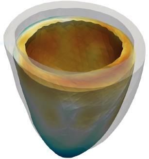
cardiac numerical simulations is seriously hampered by their overwhelming computational cost. As
a matter of fact, the simulation of a single heartbeat for an anatomically accurate patient-specific
model may require several hours of computational time even on a supercomputer platform.
    A promising approach to address this issue is to replace the computationally expensive car-
diac electromechanical model, say the full-order model (FOM), with a reduced version of it, called
reduced-order model (ROM), to be called any time new parameters come in. In the so-called offline
phase, the ROM is built from a database of numerical simulations that are previously obtained by
solving the FOM itself. Then, in the online phase, the ROM is used as a surrogate of the FOM, at
a dramatically reduced computational cost, for any new instance of the parameters. Clearly, this
procedure pays off if the computational gain of the online phase outweighs the cost of the offline
phase, or whenever the online phase requires real-time execution, which is often the case in the
clinical practice, where timeliness is a key factor.
    Recently, this framework has been applied in the context of cardiac modeling, primarily by
using machine learning algorithms, including Gaussian Process emulators (GPEs), Artificial Neural
Networks (ANNs), decision tree algorithms such as eXtreme Gradient Boosting (XGBoost) and K-
Nearest Neighbor (KNN) [7, 10, 11, 13, 31]. These emulators are trained to fit the map that links
the model parameters with a set of scalar outputs of interest, known as quantities of interest (QoIs),
which represent clinically meaningful biomarkers. This map is learned from a collection of numerical
simulations, obtained by sampling the parameter space, which can then be used as FOM surrogate.
    Replacing a FOM with a ROM is particularly advantageous in the so-called many-query settings,
i.e. when the forward model has to be solved many times for different parameter values. This is
the case, for example, of parameter calibration [6, 22] and sensitivity analysis [28, 43, 56, 67],
fundamental tools for a reliable use of computational models in the clinical practice. In fact, only
a few of the many parameters feeding cardiac electromechanical models can be directly measured,
while most of them must be estimated through indirect (possibly non-invasive) measurements, by
solving suitable (typically ill-posed) inverse problems [2]. It is therefore important to quantify how
much each parameter affects the outputs of the model and, vice versa, how uncertainty on measured
data reverberates on parameter uncertainty. These requirements are at the basis of the verification
and validation under uncertainty (VVUQ) paradigm [25, 36] and are often necessary to comply with
standards issued by health agencies and policy makers, such as the ASME V&V40 standard [1]
recognized by the FDA [14].
    In this paper, we propose a machine learning method to build ROMs of cardiac electromechanical
models. Our approach relies on the ANN-based method that we proposed in [47], which can learn
a time-dependent differential equation from a collection of input-output pairs. With respect to
existing approaches, we only surrogate the time-dependent pressure-volume relationship of a cardiac
chamber, while we do not reduce the model describing external circulation. The latter is indeed
either a low dimensional 0D windkessel or closed-loop circulation model comprised of few state
variables (up to two dozens), which does not require further reduction. In other terms, we derive
an ANN-based ROM for the computationally demanding 3D components, while we leave in FOM
version the lightweight ones. Unlike emulators, for which the online phase consists in evaluations
of the map linking model parameters to QoIs, with our approach the online phase consists instead
in numerical simulations, in which the ANN-based ROM of the electromechanical model is coupled
with the circulation model, at a very low computational cost. As a matter of fact, these numerical
simulations can be performed in real-time on a standard laptop.
    We consider two different test cases to prove the efficacy of our mathematical approach. We
perform variance-based global sensitivity analysis on both electromechanical and hemodynamic pa-
rameters and Bayesian estimation by means of the Markov Chain Monte Carlo (MCMC) method to
infer two parameters from noisy measurements of two scalar outputs.

                                                  2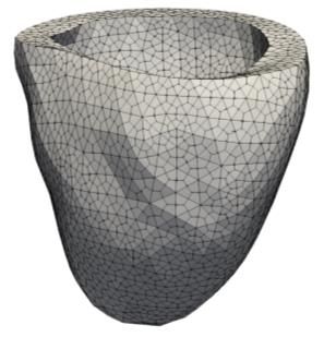
This paper is organized as follows. In Sec. 2 we present the proposed method and the models
used to produce the numerical results, which are presented and commented in Sec. 3. Then, in
Sec. 4, we critically discuss the obtained results and the pros and cons of the proposed method,
with respect to other methods available in the literature. Finally, we draw our conclusions and final
remarks in Sec. 5.
This manuscript is accompanied by https://github.com/FrancescoRegazzoni/cardioEM-learning,
a public repository containing the codes and the datasets necessary to reproduce the presented re-
sults.
2 Methods
We introduce our method in an abstract formulation for cardiac electromechanics. As a matter of
fact, our approach, thanks to its non-intrusive nature, can be applied to different electromechanical
models that are available in literature.
2.1 The full-order model (FOM)
Let us consider a generic model of cardiac electromechanics, that is a set of differential equations
describing physical processes involved in the heart function. We introduce the state vector y(t),
collecting the state variables associated with this multiphysics system. These may include the
transmembrane potential, gating variables, ionic concentrations, protein states, tissue displacement,
or simply phenomenological variables. In this paper, we focus on the single-chamber case of the
human heart (e.g. the left ventricle, that we call from now on LV), as the generalization to multiple
chambers is straightforward. By introducing a nonlinear differential operator L that encodes the
differential equations and boundary conditions associated with the electromechanical model, the
latter reads
∂y(t) = L(y(t), p (t), t; p ) for t ∈ (0, T ],
LV M
∂t (1)
y(0) = y0 ,
where pLV (t) denotes the LV endocardial pressure (here seen as an input), pM are the model pa-
rameters (possibly including, e.g., electrical conductivities, cell membrane conductances, protein
binding affinities, contractility, passive tissue properties) and y0 is the initial state. We denote by
PM ⊆ RNM the space of parameters such that pM ∈ PM , being NM the number of parameters.
We notice that the right-hand side of (1) depends on t, as heartbeats are paced by externally applied
stimuli that we assume to have a period of duration THB , which is fixed a priori.
The 3D cardiac electromechanical model (1), henceforth denoted by M3D , must be coupled with
a closure relationship assigning the pressure pLV (t). One possible option is to couple the M3D model
with a 0D model for the external circulation (see e.g. [3, 21, 50]), thus obtaining a system in the
form of
∂y(t)
= L(y(t), pLV (t), t; pM ) for t ∈ (0, T ],
∂t
dc(t)
= f (c(t), pLV (t), t; pC ) for t ∈ (0, T ],
dt (2)
0D 3D
VLV (c(t)) = VLV (y(t)) for t ∈ (0, T ],
y(0) = y0 ,
c(0) = c0 ,
3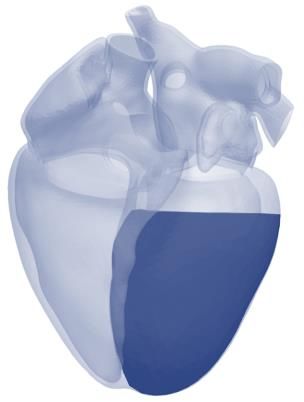
Left Ventricle                          Heart geometry
                                                                              mesh

                                                                                     Simulation results
                                                                                           110                                 100

                                                                                           activation time [ms]

                                                                                                                              active stress [kPa]
                                                                                             0                                   0
                                                                               pressures                            volumes

Figure 1: The M3D -C model. The parameters pC and pM (left) are associated with the C and M3D
respectively. The two mathematical models are coupled via the variables pLV and VLV . Their union
constitutes the model M3D -C. The model M3D -C that we consider to produce the numerical results
of this paper is shown in the center of the figure. For more details on the M3D -C model and for
the definition of the parameters pC and pM , see Sec. 2.6. The 3D Finite Element model requires
a computational mesh, obtained from the patient’s heart geometry (top right). The output of the
numerical simulations (bottom right) consists in spatially distributed fields (such as activation time,
active tension and tissue displacement) and in 0D transients (such as pressures and volumes).

where c(t) are the state variables of the circulation model (pressures, volumes and fluxes in the
circulatory network) and pC ∈ PC ⊆ RNC is a vector of NC parameters (e.g. vascular resistances
and conductances). The mechanical and hemodynamic models are coupled through the geometric
                            3D            0D
consistency relationship VLV   (y(t)) = VLV  (c(t)), where the left-hand and right-hand sides represent
the LV volume predicted by the M3D and by the C models, respectively. The LV pressure pLV
is determined as a Lagrange multiplier that enforces the consistency relationship. An alternative
approach is to adopt different closure relationships in the different phases of the heartbeat [19, 30]
with suitable preload and afterload models, such as windkessel models [65]. These relationships link
                                                                          3D
the changes in LV pressure pLV with its volume, obtained as VLV = VLV        (y). In both cases, should
the M3D be coupled to a closed-loop circulation model or to an afterload-preload relationship, we
denote by M3D -C the resulting coupled model. In Fig. 1 we show an M3D -C model in which C
consists of a the lumped-parameter closed-loop model of [50], which is employed to produce the
numerical results of Sec. 3.
    We remark that the closure relationships never directly involve the state y of the model M3D ,
                                   3D
but only the LV volume VLV = VLV      (y). This is a key observation since it suggests that a ROM that
is able to surrogate the relationship between pLV and VLV , albeit agnostic of the state y, can replace
the M3D model in its coupling to the C model. In what follows, we present our strategy to build an
ANN-based ROM of the M3D model, denoted by MANN , which can be coupled with the C model
resulting in the MANN -C coupled model, that will surrogate the M3D -C model.

                                                  4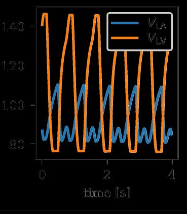
2.2 The reduced-order model (ROM)
To setup a ROM surrogating the M3D model of Eq. (1), we employ the machine learning method that
we proposed in [47]. This method is designed to learn a differential equation from time-dependent
input-output pairs, by training an Ordinary Differential Equation (ODE) model, whose right-hand
side is represented by an ANN. In this work, we define our ANN-based ROM MANN as
dz(t) = N N z(t), p (t), cos( 2πt ), sin( 2πt ), p ; w
LV THB THB M b for t ∈ (0, T ],
dt (3)
z(0) = z0 ,
where z(t) ∈ RNz is the reduced state and N N : RNz +NM +3 → RNz is a fully connected ANN. The
ANN input consists indeed of Nz state variables, NM scalar parameters, the pressure pLV , and the
two periodic inputs cos(2πt/THB ) and sin(2πt/THB ) (whose role will be clarified later), for a total
of Nz + NM + 3 input neurons. The vector w b ∈ RNw encodes the weights and biases of the ANN,
that need to be suitably trained. We remark that, among the arguments of the ANN, we have not
introduced the time variable t, but rather cos(2πt/THB ) and sin(2πt/THB ), that are the coordinates
of a point cyclically moving along a circumference with period THB . In this way, the ROM encodes
by construction the periodicity associated with the heartbeat pacing. This expedient allows for the
use of the ROM also for time spans longer than those shown during the training phase. Moreover,
by introducing the parametric dependence (i.e. on pM ) within the ANN, the latter is not specific
to a particular parameter setting.
In this work, according to [47], we adopt an output-inside-the-state approach, that is we train
the model so that the LV volume coincides with the first state variable. More precisely, the LV
ANN
volume predicted by the MANN model is by definition VLV (z(t)) := z(t) · e1 , where e1 is the first
Nz
element of the canonical basis of R . Therefore, the first ROM state variable has a clear physical
interpretation (i.e. it coincides with the LV volume), while the other ROM states are latent variables
with no immediate physical interpretation, providing however a compact representation of the full-
3D
order state y(t). Coherently with this choice, we define the initial state as z0 = (VLV (y0 ), 0)T . The
remaining initial states are set, without loss of generality, to zero (this choice does not reduce the
space of candidate models, as proved in [47]).
Here we need to determine the optimal value of the weights w, b such that the MANN model
reproduces the outputs of the M3D model as accurately as possible. With this goal, we generate
a training set, by sampling the parameter space PM × PC with Ntrain sample points. For each
sample, we perform a simulation with the M3D -C model until time Ttrain , and we record the LV
pressure and volume transients. The training set is thus given by
piC , piM , piLV (t), VLV
i
(t) t ∈ [0, Ttrain ], for i = 1, . . . , Ntrain .
We remark that, due to the non-intrusive nature of our method, there is no need to retain the
FOM states y(t). Finally, we train the ANN weights w b by minimizing the discrepancy between the
training data and the model outputs, that is by considering the following constrained optimization
problem
"N #
Xtrain Z Ttrain
i ANN i 2 2
w
b = argmin |VLV (t) − VLV (z (t))| dt + β|w|
w∈RNw i=1 0
such that, for each i = 1, . . . , Ntrain :
(4)
i
dz (t)
= N N zi (t), piLV (t), cos( T2πt ), sin( T2πt ); piM ; w
for t ∈ (0, Ttrain ],
dt
HB HB
i
z (0) = z0 ,
5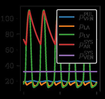
parameter space                                                                             training
                                                                                                  dataset
                                parameter space sampling

                                                                 pLV [mmHg]
                              (training dataset generation)

                                                                                           VLV [mL]

                                                                 pLV [mmHg]
                                                                                                             training

                                                    simulation
                                                                      VLV [mL]

                                                                              surrogates

Figure 2: Training pipeline of the MANN model. First, we sample the parameter space PM × PC
(top left figure) and, for each parameter instance (pM , pC ), we simulate some heartbeats through
the M3D -C model (center figure). Finally, from the training set obtained by collecting the resulting
pressure and volume transients (top right figure), we train the ANN-based model MANN (bottom
right figure), according to Eq. (4).

where β > 0 is a regularization hyperparameter. We remark that the optimization problem (4) is
not a standard machine learning problem of data fitting. Indeed, the ANN appears at the right-hand
side of a differential equation that acts as a constraint under which the loss function is minimized.
To train this model, we use the algorithm proposed in [47], which envisages approximating the
differential equation by the Forward Euler method, the loss function by the trapezoidal method, and
then computing the gradients by solving the adjoint equations. The parameters are then optimized
by means of the Levenberg-Marquardt method [35]. The training pipeline is summarized in Fig. 2.
    Once the ANN has been trained (that is, the optimal weights w     b have been determined), the
MANN model can be used as a surrogate of the M3D model, also for different combinations of the
parameters than those contained in the training set. Moreover, it can be coupled with the closure
relationships C, thus obtaining the MANN -C model. For example, by considering the case of a

                                                        6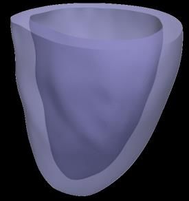
pressure-volume transients
simulation extraction
or
Figure 3: Parameters-to-QoIs computation using either the M3D or the MANN model. Given a
parameter instance (pM , pC ), either the M3D or the MANN model can be coupled with the C model
to obtain pressure and volume transients, from which a set of QoIs are extracted. See Tabs. 1, 2
and 3 for the definition of pM , pC and q, respectively.
closed-loop circulation model, as in (2), its reduced counterpart MANN -C reads
dz(t)
= N N z(t), pLV (t), cos( T2πt ), sin( 2πt
THB ); pM ; w
b for t ∈ (0, T ],
dt HB
dc(t)
= f (c(t), pLV (t), t; pC ) for t ∈ (0, T ],
dt (5)
0D ANN
VLV
(c(t)) = VLV (z(t)) for t ∈ (0, T ],
z(0) = z0 ,
c(0) = c0 .
As matter of fact, the M3D model has the same input-output structure of the model being surrogated,
that is MANN . Hence, the latter can be employed in replacement of the former in approximating
the outputs associated with a given set of parameters (pM , pC ), as shown in Fig. 3.
2.3 Hyperparameters tuning
Like any machine learning algorithm, our method depends on a set of hyperparameters, that is
variables that are not trained (they are not part of the vector w),b but are used to control the
training process. These include ANN architecture hyperparameters (namely the number of layers
Nlayers and the number of neurons per layer Nneurons ), the regularization factor β and the number
7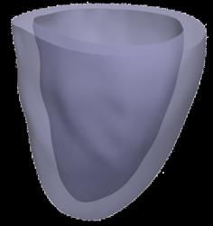
of reduced states Nz . To tune the hyperparameters, we rely on a k-fold cross-validation procedure.
Specifically, after splitting the training set into k = 5 non-overlapping subsets, we cyclically train
the model by excluding one subset that is used as validation set. Finally, we evaluate the average
validation errors and we select the hyperparameters setting that attains the lowest validation error
and better generalization properties (see Appendix A.4 for more details).

2.4    Global sensitivity analysis
To assess how much each parameter contributes to the determination of a QoI, e.g. a biomarker
of clinical interest, we perform a global sensitivity analysis. This is typically done by sampling the
parameter space and by computing suitable indicators, such as Borgonovo indices [43], Sobol indices
[24, 56], Morris elementary effects [34], ANCOVA indices [67] and Kucherenko indices [28]. In this
work, we perform a variance-based sensitivity analysis, which relies on a probabilistic approach. We
compute Sobol indices to quantify the sensitivity of a QoI (say qj ) with respect to a parameter
(say pi ). Specifically, the so-called first-order Sobol index (denoted by Sij ) indicates the impact on
the j-th QoI (i.e. qj ) of the i-th parameter (i.e. pi ) when the latter varies alone, according to the
definition
                                                Varpi [Ep∼i [qj |pi ]]
                                         Sij =                         ,
                                                     Var [qj ]
where p∼i indicates the set of all parameters excluding the i-th one. The first-order Sobol index Sij ,
however, only accounts for the variations of the parameter pi alone, averaged over variations in the
other parameters, and thus does not account for the interactions among parameters. Conversely, it
is possible to assess the importance of a parameter in determining a QoI, also accounting for the
                                                                                        T
interactions among parameters, by resorting to the so-called total-effect Sobol index Sij , defined as

                       T      Ep∼i [Varpi [qj |p∼i ]]     Varp∼i [Epi [qj |p∼i ]]
                      Sij =                           =1−                         .
                                    Var [qj ]                  Var [qj ]
The latter index quantifies the impact of a given parameter when it varies alone or together with
other parameters [56].
    To compute an estimate of the Sobol indices, we use the Saltelli method [24, 53], that makes
use of Sobol quasi-random sequences to approximate the integrals that need to be computed. In
practice, this method requires evaluating the model for a large number of parameters, and then
processing the obtained QoIs to provide an estimate of the Sobol indices.
    In this paper we perform a variance-based global sensitivity analysis simultaneously with respect
to the circulation model parameters pC and the electromechanical model parameters pC (that is, we
set p = (pM , pC )). To this end, we use model MANN -C as a surrogate for model M3D -C to perform
the evaluations required by the Saltelli method. As we will see in Sec. 3, using MANN -C instead
of M3D -C entails a huge computational gain. In addition, for each parameter setting we simulate
a certain number of heartbeats to achieve a limit cycle (i.e. a periodic solution), and we calculate
QoIs with respect to the last cycle, which is the most significant one (as it removes the effects
of incorrect initializations of the state variables). We remark that the need to simulate a certain
number of heartbeats to overpass the transient phase (that typically lasts from 5 to 15 cycles, see
Appendix A.2) makes the use of a reduced cardiac electromechanical model even more necessary.

2.5    Parameter estimation under uncertainty
The patient-specific personalization of a cardiac electromechanical model requires, besides the usage
of a geometry derived from imaging data, the estimation of the parameters associated with the

                                                    8
mathematical model (or at least the most important ones), starting from clinical measurements.
Very often, only a few scalar quantities are available for this purpose; moreover, the resolution of
this inverse problem (i.e. estimating p from q) should account for the noise that unavoidably affects
the measurement of q and that reflects in uncertainty on p.
Bayesian methods, such as MCMC [6] and Variational Inference [22], permit to address these
issues within a rigorous statistical framework, by providing the likelihood, expressed as a probability
distribution of the parameters values, given the observed QoIs (denoted by qobs ). Unlike methods
that provide point estimates, either based on gradient-descent [35] or genetic [23] optimization
algorithms, Bayesian methods are able to provide a probability distribution on the parameter space,
encoding the credibility of each parameter combination. The credibility computation accounts for
the uncertainty on measurements (associated with measurement noise and encoded in the noise
covariance matrix Σ), as well as a prior distribution on parameters (denoted by πprior (p)), that is
previous knowledge or belief about the parameters. By denoting the parameters-to-QoIs map by
F : p 7→ q, we have qobs = F(p) + , where ∼ N (·|0, Σ) denotes the measurement error (that
we assume for simplicity to be distributed as a Gaussian random variable). Bayes’ theorem states
that the posterior distribution of parameters, that is the degree of belief of their value after having
observed qobs , is given by
1
πpost (p) = N (qobs |F(p), Σ) πprior (p),
Z
where the normalization constant Z is defined as
Z
Z= N (qobs |F(b
p), Σ) dπprior (b
p).
P
In practice, the computation of πpost may be challenging from the computational viewpoint, because
of the need to approximate the integral that defines Z. The MCMC method permits to approximate
the distribution πpost with a relatively small computational effort. Similarly to the Saltelli method
that we use for sensitivity analysis, also the MCMC method requires a large number of model
evaluations, for different parameter values. Moreover, this method is non intrusive, that is it only
requires evaluations of the map F : p 7→ q. Therefore, we can employ for this purpose the MANN -C
model as a surrogate for the M3D -C model, which drastically reduces the necessary computational
time.
Moreover, we remark that the Bayesian framework permits to rigorously account for the approx-
imation error introduced by replacing the high fidelity model M3D -C by its surrogate MANN -C.
Indeed, if we denote by Fe the approximated parameters-to-QoIs map represented by the surrogate
model MANN -C, we have F(p) = F(p) e + ROM , where ROM is the ROM approximation error. It
follows qobs = F(p)
e + ROM + exp , where exp is the experimental measurement error. Since the
two sources of error can be assumed independent, the covariance of the total error = ROM + exp
satisfies Σ = ΣROM + Σexp , where ΣROM is the ROM approximation error covariance (which can
be estimated by evaluating the ROM on a testing set) and Σexp is the experimental error covariance
(that depends on the measurement protocol at hand). This permits to take into account in the
estimation process the error introduced by the surrogate model.
To assess the capability of our ROM to accelerate the estimation of parameters for multiscale
cardiac electromechanical models, we perform the following test. First, we perform a simulation with
the M3D -C model, from which we derive a set of QoIs (qobs ). Then, by employing the MANN -C
model as a surrogate of the M3D -C model, we obtain a Bayesian estimate of the parameters, that
we validate against the values used to generate qobs .
9Parameter Baseline Unit Description
aXB 160.0 MPa Cardiomyocytes contractility
σf 76.43 mm s−1 Electrical conductivity along fibers
α 60.0 degrees Fibers angle rotation
C 0.88 kPa Passive stiffness
Table 1: Parameters pM of the M3D model considered in this work and associated baseline values.
2.6 The cardiac electromechanical model
As mentioned above, due to its non-intrusive nature, our method is not limited to a specific cardiac
electromechanical model, but can be applied to virtually any electromechanical model as long as
pressure and volume transients are available for the training procedure. In this section, we briefly
introduce the specific model used to produce the numerical results of this paper.
We consider a LV geometry processed from the Zygote 3D heart model [27] endowed with a
fiber architecture generated by means of the Bayer-Blake-Plank-Trayanova algorithm [4, 42]. Before
starting the simulations, we recover the reference unstressed configuration through the algorithm that
we proposed in [50]. To model the action potential propagation, we employ the monodomain equation
[8], coupled with the ten Tusscher-Panfilov ionic model [60]. We model the microscale generation
of active force through the biophysically detailed RDQ20-MF model [46], that is coupled, within
an active stress approach, with the elastodynamics equations describing tissue mechanics. On the
other hand, the passive behavior of the tissue is modeled through a quasi-incompressible exponential
constitutive law [61]. We model the interaction with the pericardium by means of spring-damper
boundary conditions at the epicardium, while we adopt energy-consistent boundary conditions [48]
to model the interaction with the part of the myocardium beyond the artificial ventricular base. To
model blood circulation, that is C, we rely on the 0D closed-loop model presented in [50], consisting of
a compartmental description of the cardiac chambers, systemic and pulmonary, arterial and venous
circulatory networks, based on an electrical analogy. The different compartments are modeled as
RLC (resistance, inductance, capacitance) circuits, while cardiac valves are described as diodes.
Among the parameters associated with the M3D model, in this work we focus on the four ones
reported in Tab. 1. Similarly, we report in Tab. 2 the parameters associated with the C model.
We report in Tab. 3 the list of all the QoIs, computed from the solution of the M3D -C model, and
outputs of interest that are used through this paper. The last column of the table indicates which
variables are used for cross-validation during the training phase (see Sec. 2.3), those that are used
for sensitivity analysis purposes (see Sec. 2.4) and those that are used to run Bayesian parameter
estimations (see Sec. 2.5).
To numerically approximate this multiphysics and multiscale model, we adopt the segregated
approach proposed in [51], by which the subproblems are solved sequentially. For space discretiza-
tion, we rely on bilinear Finite Elements defined on hexahedral meshes, adopting a different spatial
resolution for the electrophysiological and the mechanical variables. For time discretization, we
employ a staggered scheme, where different time steps are used according to the specific subprob-
lem. Moreover, to avoid the numerical oscillations arising from the mechanical feedback on force
generation (that are commonly cured by recurring to a monolithic scheme [30, 40]), we use the
stabilized-staggered scheme that we proposed in [52]. This numerical model requires, on a 32 cores
computer platform, nearly 4 hours of computational time to simulate a heartbeat. More details on
the numerical discretization and the computational platform employed to generate the training data
10Parameter Baseline Unit Description
tot
Vheart 400.15 mL Initial blood pool volume of the heart
act act act
ELA , ERA , ERV 0.07, 0.06, 0.55 mmHg mL−1 LA/RA/RV active elastance
pass pass pass
ELA , ERA , ERA 0.18, 0.07, 0.05 mmHg mL−1 LA/RA/RV passive elastance
contr contr contr
TLA , TRA , TRV 0.14, 0.14, 0.20 s LA/RA/RV contraction time
rel rel rel
TLA , TRA , TRV 0.14, 0.14, 0.32 s LA/RA/RV relaxation time
V0,LA , V0,RA , V0,RV 4.0, 4.0, 16.0 mL LA/RA/RV reference volume
tav av
L , tR 0.16, 0.16 s Left/Right atrioventricular delay
Rmin , Rmax 0.0075, 75006.2 mmHg s mL−1 Valve minimum/maximum resistance
SYS SYS
RAR , RVEN 0.64, 0.32 mmHg s mL−1 Systemic arterial/venous resistance
PUL PUL
RAR , RVEN 0.032, 0.036 mmHg s mL−1 Pulmonary arterial/venous resistance
SYS SYS
CAR , CVEN 1.2, 60.0 mL mmHg−1 Systemic arterial/venous capacitance
PUL PUL
CAR , CVEN 10.0, 16.0 mL mmHg−1 Pulmonary arterial/venous capacitance
SYS SYS
LAR , LVEN 0.005, 0.0005 mmHg s2 mL−1 Systemic arterial/venous inductance
LPUL PUL
AR , LVEN 0.0005, 0.0005 mmHg s2 mL−1 Pulmonary arterial/venous inductance
Table 2: Parameters pC of the C model considered in this work and associated baseline values (LA
= left atrium; RA = right atrium; RV = right ventricle).
Parameter Unit Description Usage
Left Atrium
min max
VLA , VLA mL End-systolic and end-diastolic volume GSA
min max
pLA , pLA mmHg Minimum and maximum pressure GSA
Left ventricle
VLV (t) mL Volume transient X-validation
pLV (t) mmHg Pressure transient X-validation
min max
VLV , VLV mL End-systolic and end-diastolic volume X-validation, GSA
min max
pLV , pLV mmHg Minimum and maximum pressure X-validation, GSA
max min
SVLV mL Stroke volume (VLV − VLV ) X-validation, GSA
Right Atrium
min max
VRA , VRA mL End-systolic and end-diastolic volume GSA
pmin max
RA , pRA mmHg Minimum and maximum pressure GSA
Right ventricle
min max
VRV , VRV mL End-systolic and end-diastolic volume GSA
min max
pRV , pRV mmHg Minimum and maximum pressure GSA
max min
SVRV mL Stroke volume (VRV − VRV ) GSA
Systemic arterial circulation
pmin max
AR,SYS , pAR,SYS mmHg Minimum and maximum pressure GSA, MCMC
Table 3: List of QoIs used through this paper, either for cross-validation (X-validation), global
sensitivity analysis (GSA) or MCMC based Bayesian parameter estimation (MCMC).
11used in this paper are available in Appendix A.1.
2.7 Software libraries
The cardiac electromechanics simulations considered in this paper are performed by means of the
lifex library1 , a high-performance C++ platform developed within the iHEART project2 . To train
the ANN-based models, we employ the open source MATLAB library model-learning3 , that im-
plements the machine learning method proposed in [47] and used in this paper. Sensitivity analysis
is carried out through the open source Python library SALib4 [20]. Finally, for the MCMC based
Bayesian parameter estimation we rely on the open source Python library UQpy5 [37]. To employ the
ANN-based models trained with the MATLAB library model-learning within the Python environ-
ment of SALib and UQpy, we exploit pyModelLearning, a Python wrapper for the model-learning
library, which is available in its GitHub repository6 .
Both the MATLAB codes that are used to train the ANN-based ROMs and the datasets that per-
mit to reproduce the numerical results are publicly available in the online repository accompanying
this manuscript7 .
3 Results
3.1 Trained models
To generate the pressure and volume transients needed to train an ANN-based ROM, we sample
the parameter space PM × PC with a Monte Carlo approach, even if more sophisticated sampling
strategies – such as Latin Hypercube Design – can be considered as well. For simplicity, in this stage
we only consider a subset of the parameters pC , selected as the most significant ones, on the basis of
a preliminary variance-based global sensitivity analysis, obtained with a version of the closed-loop
model in which the LV is also represented by a 0D circuit element (see Appendix A.3).
We consider two scenarios. First, we study the variability with respect to a single parameter,
namely the active contractility. Thus, we set pM = [aXB ]. Under this setting, we generate 30
numerical simulations through the M3D -C model to train a ROM, henceforth denoted by Msingle ANN .
For this ROM, the remaining parameters (i.e. σf , α and C) are kept constant (more precisely, equal
to the baseline values of Tab. 1). Then, we consider the full parametric variability (that is, we
set pM = [aXB , σf , α, C]), we generate 40 training samples and we train a second ROM, denoted
by Mfull
ANN . All the numerical simulations included in the training set are 5 heartbeats long. The
optimal sets of hyperparameters, tuned through the algorithm of Sec. 2.3, are reported in Tab. 4. In
both the considered cases, training an ANN-based model takes approximately 18 hours on a single
core standard laptop.
Once trained, the two ROMs (Msingle full
ANN and MANN ) can be coupled with the circulation model C,
single full
thus obtaining the models MANN -C and MANN -C, according to Eq. (5). These two models represent
two surrogates of the M3D -C model, capable of approximating its output at a dramatically reduced
1
https://lifex.gitlab.io
2
iHEART - An Integrated Heart Model for the simulation of the cardiac function, European Research Council
(ERC) grant agreement No 740132, P.I. Prof. A. Quarteroni
3
https://model-learning.readthedocs.io/
4
https://salib.readthedocs.io/
5
https://uqpyproject.readthedocs.io/
6
https://github.com/FrancescoRegazzoni/model-learning
7
https://github.com/FrancescoRegazzoni/cardioEM-learning
12Trained model Parameters Training set size Hyperparameters
pM Ntrain Nz Nlayers Nneurons β
Msingle
ANN [aXB ] 30 2 1 8 0
Mfull
ANN [aXB , σf , α, C] 40 1 1 12 0.01
Table 4: Optimal sets of hyperparameters for the two trained models Msingle full
ANN and MANN .
computational cost. As a matter of fact, numerical simulations with either the Msingle
ANN or the MANN
full
model take nearly one second of computational time per heartbeat on a single core standard laptop.
To test the accuracy of the Msingle full
ANN -C and MANN -C models with respect to the M3D -C model,
we consider a testing dataset, by taking unobserved samples in the parameter space PM × PC . For
both models, we consider 15 testing simulations of the same duration of the ones included in the
training set. In addition, to test the reliability of the ROMs over a longer time horizon than the one
considered in the training set, we include in the testing set 5 simulations of double length (i.e. 10
heartbeats). Then, we compare the simulations obtained with the two ROMs (Msingle full
ANN and MANN )
with the ones obtained with the M3D -C model for the same parameters pM and pC .
The accuracy of the two ROMs is summarized Tabs. 5 and 6. Specifically, in Tab. 5 we report
metrics regarding the ability of the ROMs to correctly predict the function of the LV, that is the
chamber surrogated by the ANN-based model. Specifically, we report the relative errors in L2 norm
(i.e. the mean square errors) associated with pressure and volume transients (pLV and VLV ) and
the relative errors on some biomarkers of clinical interest (maximum and minimum pressures and
volumes). For the latter, we also report the coefficient of determination R2 . We notice that both
model Msingle full
ANN -C and model MANN -C are able to surrogate model M3D -C with remarkably good
accuracy. Model MANN -C features slightly larger errors than model Msingle
full
ANN -C; this is not surprising
since model Mfull
ANN -C explores a much larger parametric space than model Msingle
ANN -C (four parameters
instead of one). Interestingly, the errors obtained over a long time horizon are very similar to those
obtained for simulations of the same duration as those used to train the ANNs. This demonstrates
the reliability of the ROMs in long-term simulations. Similarly, in Tab. 6 we report the errors and
R2 coefficients associated with the RV output (for simplicity, we here consider only 5 heartbeats long
simulations). The accuracy obtained in reproducing the RV function is even better than that for the
LV, coherently with the fact that the RV is included in the C model and thus it is not surrogated
by the ANN-based model.
In Figs. 4 and 5 we compare 10 heartbeats long transients obtained with the Msingle ANN -C and
full
MANN -C models, respectively, to those obtained with the M3D -C model. All these transients were
not used to train the ANN-based models (that is, they belong to the testing set). In Fig. 6 we show
the LV biomarkers predicted by the Msingle full
ANN -C and MANN -C models versus those predicted by the
M3D -C model.
3.2 Coupling the electromechanical reduced-order model with different
circulation models
To generate the data used to train the MANN model, we employ the M3D -C coupled model (that
is, we couple the M3D model with the circulation model C). However, the ANN-based ROM MANN
surrogates the M3D model regardless of its coupling with a specific circulation model. In fact, thanks
to Eq. (5), the trained MANN model can be coupled with circulation models that are different from
135 heartbeats
pLV (t) VLV (t) pmin
LV pmax
LV
min
VLV max
VLV
relative error 0.0336 0.0090 0.0097 0.0046 0.0139 0.0035
Msingle
ANN -C vs M3D -C R2 99.691 99.864 99.896 99.948
relative error 0.0620 0.0285 0.0517 0.0272 0.0471 0.0127
Mfull
ANN -C vs M3D -C R2 94.370 95.302 95.942 97.061
10 heartbeats
pLV (t) VLV (t) pmin
LV pmax
LV
min
VLV max
VLV
relative error 0.0293 0.0071 0.0113 0.0037 0.0096 0.0031
Msingle
ANN -C vs M3D -C R2 99.924 99.980 99.851 99.944
relative error 0.0631 0.0265 0.0442 0.0147 0.0382 0.0122
Mfull
ANN -C vs M3D -C R2 92.227 99.957 99.229 99.063
Table 5: Testing errors and R2 coefficients on the LV outputs obtained with the two models Msingle
ANN
and Mfull
ANN , for 5 heartbeats long (top) and 10 heartbeats long (bottom) simulations.
5 heartbeats
pRV (t) VRV (t) pmin
RV pmax
RV
min
VRV max
VRV
relative error 0.0048 0.0035 0.0015 0.0027 0.0028 0.0004
Msingle
ANN -C vs M3D -C R2 [%] 100.000 99.993 99.998 100.000
relative error 0.0069 0.0040 0.0029 0.0079 0.0072 0.0069
Mfull
ANN -C vs M3D -C R2 [%] 99.994 99.807 99.819 99.997
Table 6: Testing errors and R2 coefficients on the RV outputs obtained with the two models Msingle
ANN
and Mfull
ANN , for 5 heartbeats long simulations.
14M3D -C 40
140
Msingle
ANN -C 35
120
30
100
pRV [mmHg]
pLV [mmHg]
25
80 20
60 15
40 10
20 5
0
40 60 80 100 120 140 160 50 75 100 125 150 175 200
VLV [mL] VRV [mL]
160
140
VLV [mL]
120
100
80
60
40
150
pLV [mmHg]
100
50
0
0 1 2 3 4 5 6 7 8
time [s]
Figure 4: Pressure and volume transients obtained with the MsingleANN -C (dashed lines), compared to
those obtained with the M3D -C model (solid lines). The different colors correspond to different
samples of the testing set. For the sake of clarity, only three samples are shown in the first row.
15M3D -C 50
140
Mfull
ANN -C
120
40
100
pRV [mmHg]
pLV [mmHg]
30
80
60 20
40
10
20
0
40 60 80 100 120 140 160 50 100 150 200 250
VLV [mL] VRV [mL]
175
150
VLV [mL]
125
100
75
50
150
125
pLV [mmHg]
100
75
50
25
0 1 2 3 4 5 6 7 8
time [s]
Figure 5: Pressure and volume transients obtained with the Mfull ANN -C (dashed lines), compared to
those obtained with the M3D -C model (solid lines). The different colors correspond to different
samples of the testing set. For the sake of clarity, only three samples are shown in the first row.
16Model M3D -C vs Msingle
ANN -C
pmin
LV [mmHg] pmax
LV [mmHg]
min
VLV [mL] max
VLV [mL]
25
180 180
5 heartbeats 5 heartbeats 120 5 heartbeats 5 heartbeats
10 heartbeats 10 heartbeats 10 heartbeats 10 heartbeats
20 160 105 165
140 90 150
15
120 75 135
10 100 60
120
45
5 80 105
30
5 10 15 20 25 80 100 120 140 160 180 30 45 60 75 90 105 120 105 120 135 150 165 180
Model M3D -C vs Mfull
ANN -C
pmin
LV [mmHg] pmax
LV [mmHg]
min
VLV [mL] max
VLV [mL]
25
180 180
5 heartbeats 5 heartbeats 120 5 heartbeats 5 heartbeats
10 heartbeats 10 heartbeats 10 heartbeats 10 heartbeats
20 160 105 165
140 90 150
15
120 75 135
10 100 60
120
45
5 80 105
30
5 10 15 20 25 80 100 120 140 160 180 30 45 60 75 90 105 120 105 120 135 150 165 180
Figure 6: LV biomarkers obtained with the Msingle full
ANN -C and MANN -C models versus those obtained
with the M3D -C model in the testing set. The different marker colors are associated with 5 heartbeats
and 10 heartbeats long simulations, respectively.
17pLV (t) VLV (t) pmin
LV pmax
LV
min
VLV max
VLV
Msingle
ANN -C
0
vs M3D -C 0
relative error 0.0459 0.0518 0.0065 0.0004 0.0080 0.0009
Mfull
ANN -C
0
vs M3D -C 0 relative error 0.0510 0.0219 0.0116 0.0027 0.0110 0.0063
Table 7: Testing errors on the LV outputs obtained with the two models Msingle full
ANN and MANN coupled
0
with the C model for 5 heartbeats long simulations.
the one used to generate the training data. We remind that predictions are reliable only if pressure
and volume values are inside the ranges explored during the training phase.
We demonstrate the flexibility of our approach by coupling the MANN model with a pressure-
volume closure relationship that is different from the closed-loop circulation model C used during the
training phase (see Sect. 2.6). Specifically, we consider a circulation model C 0 with a windkessel type
relationship during the ejection phase and a linear pressure ramp during the filling phase [48]. In
spite of the different nature of the two circulation models (the one used during the training and the
one used during the testing), the ANN-based ROM trained with the C model proves to be reliable
also when it is coupled with the C 0 model. Indeed, as shown in Tab. 7, the results obtained by
the MANN -C 0 coupled model approximate those of the M3D -C 0 coupled model with an excellent
accuracy. These errors are indeed comparable to the ones obtained by surrogating the MANN -C
model with the M3D -C model (see Tab. 5).
3.3 Global sensitivity analysis
Once we have verified that models Msingle full
ANN -C and MANN -C are able to reproduce the outputs of
model M3D -C with high accuracy, we use them to perform a global senstivity analysis. The aim is
to determine which of the parameters of the circulation model (pC ) and the electromechanical model
(pM ) contribute the most to the determination of a list of outputs of interest, the so-called QoIs
T
(see Tab. 3). For this purpose, we compute the Sobol indices Sij and Sij , as described in Sec. 2.4.
When replacing model M3D -C with a ROM, we can only estimate sensitivity indices with respect
to the parameters pM that were considered during the training phase. On the other hand, we can
compute sensitivity indices with respect to all parameters pC of the circulation model, even those
that were not varied during training. It would even be possible – at least in principle – to consider a
circulation model different from the one used to generate the training data. In fact, as pointed out in
Sec. 2.2, the model Msingle full
ANN and MANN surrogate the models M3D independently of the circulation
model to which it is coupled with.
We only report the results obtained by means of the most complete ROM, that is Mfull ANN -C. The
T
results are shown in Figs. 7 and 8, respectively. First, we notice that the Sij and Sij indices have only
small differences from each other. This means that the interaction among the different parameters
is less significant, in the determination of the QoIs, than the variation of the individual parameters.
Furthermore, we note that, as expected, the QoIs associated with a given chamber or compartment
are mostly determined by the parameters associated with the same region of the cardiovascular
network. However, there are some important exceptions. Indeed, the venous resistance of the
SYS
systemic circulation RVEN has a strong impact on the right heart (RA and RV), i.e. the part
SYS
of the network located immediately upstream. In addition, the systemic arterial resistance RAR
significantly impacts the maximum LV pressure. In fact, this parameter is known to contribute in
the determination of the so-called afterload [58]. We also note that total circulating blood volume
tot
Vheart has a major impact on almost all biomarkers. Conversely, the parameters associated with
18the pulmonary circulation network have a minimal impact. In addition, parameters describing the
resistance of opened and closed valves also have a very little impact. This is an interesting result,
since it shows that these parameters, chosen as a very low and very high value respectively (since for
reasons of numerical stability they cannot be set equal to zero and infinity), have virtually no impact
(at least within the ranges considered here) on the output quantities of biomechanical interest.
Regarding individual compartments, we note that variability can be explained by only a few
parameters. Specifically, atria are mainly influenced by passive stiffness and atrioventricular delay,
whereas for the RV the most relevant parameters are active and passive stiffness. As expected, the
biomarkers associated with the LV – the only chamber included in the M3D model – are mainly
influenced by the parameters pM . Among these, the most influential one is the active contractility
aXB , followed the fibers orientation α and, to a lesser extent, the passive stiffness C. Finally, the
electrical conductivity σf has a minimal impact on the biomarkers under consideration.
It is important to note that Sobol indices are affected by the amplitude of the ranges in which the
parameters are varied. In particular, the wider the range associated with a parameter, the greater
the associated Sobol indices will be, as the parameter in question potentially generates greater
variability in the QoI. Therefore, the results shown here are valid for the specific ranges we used,
which are reported in Appendix A.5.
3.4 Bayesian parameter estimation
In this section we present a further practical use of the cardiac electromechanics ROM presented
in this paper. In particular, we show that the ROM can be used to enable Bayesian parameter
estimation for the M3D -C model, which, due to the prohibitive computational cost, would not be
affordable without the use of a ROM.
First, we consider a prescribed value for the parameter vector p = (pM , pC ) (specifically, we
employ the values reported in Tabs. 1 and 2) and we run a simulation using the M3D -C model.
Based on the output of this simulation, we consider a couple of QoIs, consisting of minimum and
maximum arterial pressure (i.e. we set q = (pmin max
AR,SYS , pAR,SYS )). The choice of these two QoIs is
motivated by the fact that they are two variables that can be measured non invasively, and in fact
they are often monitored in clinical routine. We reconstruct the value of a couple of parameters,
SYS
namely the active contractility aXB and the systemic arterial resistance RAR , assuming known and
keeping fixed the values of the remaining parameters. Indeed, we aim at demonstrating that the
ROM we propose is suitable for estimating parameters of both the M3D model (such as aXB ) and
of the C model (such as RAR SYS
). Specifically, in this section we rely on the Msingle
ANN -C model.
To mimic the presence of measurement errors, we artificially add to the exact values of the QoIs
pmin max
AR,SYS and pAR,SYS a synthetic noise, with increasing magnitude. Specifically, we add an artificial
2
noise by sampling from independent Gaussian variables with zero mean and with variance σexp . We
2 2 2 2 2
consider three cases: σexp = 0 (i.e. no noise), σexp = 0.1 mmHg and σexp = 1 mmHg .
As described in Sec. 2.5, we use the MCMC method to derive a Bayesian estimate of the parame-
ters value from (possibly noisy) measurements of the minimum and maximum arterial pressure. For
both unknown parameters we employ a non-informative prior, that is a uniform distribution on the
SYS
ranges used to train the ROM (aXB ∈ [80, 320] MPa and RAR ∈ [0.4, 1.2] mmHg s mL−1 ). According
to Sec. 2.5, we set Σ = ΣROM + Σexp , where the experimental measurement error covariance is given
2
by Σexp = σexp I2 (I2 being the 2-by-2 identity matrix) and where the ROM approximation error co-
variance is estimated from its statistical distribution on the validation set as ΣROM = 0.2 mmHg2 I2 .
More details on the MCMC setup are available in Appendix A.6.
SYS
In Fig. 9 we show the posterior distribution πpost on the parameters pair (aXB , RAR ) obtained
for the three noise levels considered. We identify with a red line the 90% credibility region, that
19p m YS
S
Y
A x
x
A x
V x
A n
n
A n
V n
A x
x
A x
V x
R x
p mV
L ma
LVma
R ma
R ma
L in
LV in
R in
R in
A in
LV
,S
,S
L mi
LVmi
R mi
R mi
L a
LV a
R a
R a
A a
R
pm
pm
pm
pm
pm
pm
pm
pm
A
R
A
V
SV
SV
V
V
V
V
V
V
V
V
act
ELA 0.01 0.00 0.00 0.00 0.00 0.00 0.00 0.00 0.00 0.00 0.00 0.00 0.00 0.00 0.00 0.00 0.00 0.00 0.00 0.00
0.8
pass
ELA 0.23 0.26 0.00 0.00 0.00 0.00 0.00 0.00 0.00 0.00 0.00 0.00 0.00 0.00 0.00 0.00 0.01 0.00 0.00 0.00
contr
TLA 0.00 0.00 0.00 0.00 0.00 0.00 0.00 0.00 0.00 0.00 0.00 0.00 0.00 0.00 0.00 0.00 0.00 0.00 0.00 0.00
rel
TLA 0.00 0.00 0.00 0.00 0.00 0.00 0.00 0.00 0.00 0.00 0.00 0.00 0.00 0.00 0.00 0.00 0.00 0.00 0.00 0.00
tav
L 0.03 0.00 0.00 0.13 0.01 0.04 0.00 0.02 0.02 0.00 0.00 0.00 0.00 0.00 0.00 0.00 0.00 0.00 0.01 0.02
V0,LA 0.00 0.00 0.00 0.00 0.00 0.00 0.00 0.00 0.00 0.00 0.00 0.00 0.00 0.00 0.00 0.00 0.00 0.00 0.00 0.00
0.7
C 0.03 0.02 0.04 0.03 0.01 0.05 0.05 0.05 0.06 0.00 0.00 0.00 0.00 0.01 0.00 0.00 0.01 0.01 0.02 0.05
α 0.03 0.02 0.07 0.04 0.14 0.03 0.08 0.10 0.13 0.00 0.00 0.00 0.00 0.01 0.00 0.00 0.02 0.01 0.05 0.10
σf 0.00 0.00 0.00 0.00 0.02 0.00 0.01 0.01 0.01 0.00 0.00 0.00 0.00 0.00 0.00 0.00 0.00 0.00 0.01 0.01
aXB 0.10 0.07 0.15 0.09 0.51 0.16 0.18 0.22 0.26 0.00 0.00 0.00 0.00 0.02 0.00 0.00 0.04 0.04 0.10 0.22 0.6
act
ERA 0.00 0.00 0.00 0.00 0.00 0.00 0.00 0.00 0.00 0.04 0.03 0.05 0.01 0.00 0.00 0.01 0.00 0.00 0.00 0.00
pass
ERA 0.00 0.00 0.00 0.00 0.00 0.00 0.00 0.00 0.00 0.17 0.21 0.05 0.01 0.00 0.00 0.04 0.00 0.00 0.00 0.00
contr
TRA 0.00 0.00 0.00 0.00 0.00 0.00 0.00 0.00 0.00 0.00 0.00 0.00 0.00 0.00 0.00 0.00 0.00 0.00 0.00 0.00
rel
TRA 0.00 0.00 0.00 0.00 0.00 0.00 0.00 0.00 0.00 0.00 0.00 0.00 0.00 0.00 0.00 0.00 0.00 0.00 0.00 0.00
0.5
tav
R 0.00 0.00 0.01 0.00 0.00 0.01 0.01 0.00 0.00 0.42 0.18 0.35 0.54 0.00 0.01 0.03 0.01 0.02 0.00 0.00
V0,RA 0.00 0.00 0.00 0.00 0.00 0.00 0.00 0.00 0.00 0.00 0.00 0.00 0.00 0.00 0.00 0.00 0.00 0.00 0.00 0.00
act
ERV 0.01 0.01 0.01 0.01 0.00 0.00 0.00 0.00 0.00 0.02 0.01 0.03 0.02 0.37 0.15 0.13 0.01 0.00 0.00 0.00
pass
ERV 0.00 0.00 0.00 0.00 0.00 0.01 0.00 0.00 0.01 0.15 0.12 0.22 0.16 0.02 0.03 0.42 0.01 0.02 0.00 0.00
contr
TRV 0.4
0.00 0.00 0.00 0.00 0.00 0.00 0.00 0.00 0.00 0.00 0.02 0.00 0.00 0.00 0.00 0.00 0.04 0.00 0.00 0.00
rel
TRV 0.00 0.00 0.00 0.00 0.00 0.00 0.00 0.00 0.00 0.00 0.03 0.00 0.00 0.00 0.00 0.06 0.00 0.00 0.00 0.00
V0,RV 0.00 0.00 0.00 0.00 0.00 0.00 0.00 0.00 0.00 0.00 0.00 0.00 0.00 0.06 0.03 0.00 0.00 0.00 0.00 0.00
SYS
RAR 0.02 0.01 0.03 0.01 0.10 0.02 0.04 0.23 0.08 0.00 0.00 0.00 0.00 0.00 0.00 0.00 0.00 0.01 0.53 0.24
SYS
CAR 0.00 0.00 0.00 0.00 0.01 0.00 0.00 0.05 0.01 0.00 0.00 0.00 0.00 0.00 0.00 0.00 0.00 0.00 0.13 0.05
0.3
SYS
RVEN 0.07 0.09 0.10 0.09 0.01 0.09 0.09 0.02 0.09 0.10 0.30 0.18 0.15 0.10 0.51 0.16 0.24 0.82 0.00 0.02
SYS
CVEN 0.00 0.00 0.00 0.00 0.00 0.00 0.00 0.00 0.00 0.00 0.00 0.00 0.00 0.00 0.00 0.00 0.00 0.00 0.00 0.00
LSYS
AR 0.00 0.00 0.00 0.00 0.00 0.00 0.00 0.00 0.00 0.00 0.00 0.00 0.00 0.00 0.00 0.00 0.00 0.00 0.00 0.00
LSYS
VEN 0.00 0.00 0.00 0.00 0.00 0.00 0.00 0.00 0.00 0.00 0.00 0.00 0.00 0.00 0.00 0.00 0.00 0.00 0.00 0.00
PUL
RAR 0.00 0.00 0.00 0.00 0.00 0.00 0.00 0.00 0.00 0.00 0.00 0.00 0.00 0.00 0.00 0.00 0.00 0.00 0.00 0.00 0.2
PUL
CAR 0.00 0.00 0.00 0.00 0.00 0.00 0.00 0.00 0.00 0.00 0.00 0.00 0.00 0.01 0.00 0.00 0.00 0.00 0.00 0.00
PUL
RVEN 0.00 0.00 0.01 0.00 0.00 0.01 0.00 0.00 0.01 0.00 0.00 0.00 0.00 0.00 0.00 0.00 0.00 0.00 0.00 0.00
PUL
CVEN 0.00 0.00 0.00 0.00 0.00 0.00 0.00 0.00 0.00 0.00 0.00 0.00 0.00 0.00 0.00 0.00 0.00 0.00 0.00 0.00
LPUL
AR 0.00 0.00 0.00 0.00 0.00 0.00 0.00 0.00 0.00 0.00 0.00 0.00 0.00 0.00 0.00 0.00 0.00 0.00 0.00 0.00 0.1
LPUL
VEN 0.00 0.00 0.00 0.00 0.00 0.00 0.00 0.00 0.00 0.00 0.00 0.00 0.00 0.00 0.00 0.00 0.00 0.00 0.00 0.00
Rmin 0.00 0.00 0.00 0.00 0.00 0.00 0.01 0.00 0.00 0.01 0.01 0.01 0.01 0.00 0.00 0.01 0.03 0.00 0.00 0.00
Rmax 0.00 0.00 0.00 0.00 0.00 0.00 0.00 0.00 0.00 0.00 0.00 0.00 0.00 0.00 0.00 0.00 0.00 0.00 0.00 0.00
tot
Vheart 0.39 0.45 0.53 0.52 0.15 0.53 0.49 0.27 0.31 0.04 0.07 0.06 0.05 0.32 0.24 0.11 0.55 0.03 0.14 0.26
0.0
Figure 7: First-order Sobol indices Sij computed by exploiting the Mfull ANN -C model. Each row
corresponds to a parameter of either the electromechanical model (i.e. pM , see Tab. 1) or the
circulation model (i.e. pC , see Tab. 2). Each column corresponds to a QoI (i.e. q, see Tab. 3). Both
parameters and QoIs are split into a number of groups, separated by a black solid line. Specifically,
from left to right, we list QoIs referred to LA, LV, RA, RV and systemic circulation. Similarly, from
top to bottom, we list parameters associated with LA, LV, RA, RV, systemic circulation, pulmonary
circulation, valves and blood total volume.
20p m YS
S
Y
A x
x
A x
V x
A n
n
A n
V n
A x
x
A x
V x
R x
p mV
L ma
LVma
R ma
R ma
L in
LV in
R in
R in
A in
LV
,S
,S
L mi
LVmi
R mi
R mi
L a
LV a
R a
R a
A a
R
pm
pm
pm
pm
pm
pm
pm
pm
A
R
A
V
SV
SV
V
V
V
V
V
V
V
V
act
ELA 0.01 0.00 0.00 0.01 0.00 0.00 0.00 0.00 0.00 0.00 0.00 0.00 0.00 0.00 0.00 0.00 0.00 0.00 0.00 0.00
pass
ELA 0.26 0.28 0.00 0.01 0.00 0.00 0.00 0.00 0.00 0.00 0.00 0.00 0.00 0.00 0.00 0.00 0.01 0.00 0.00 0.00 0.8
contr
TLA 0.00 0.00 0.00 0.00 0.00 0.00 0.00 0.00 0.00 0.00 0.00 0.00 0.00 0.00 0.00 0.00 0.00 0.00 0.00 0.00
rel
TLA 0.00 0.00 0.00 0.00 0.00 0.00 0.00 0.00 0.00 0.00 0.00 0.00 0.00 0.00 0.00 0.00 0.00 0.00 0.00 0.00
tav
L 0.04 0.01 0.01 0.16 0.01 0.04 0.00 0.02 0.03 0.00 0.00 0.00 0.00 0.01 0.00 0.00 0.00 0.00 0.01 0.02
V0,LA 0.00 0.00 0.00 0.00 0.00 0.00 0.00 0.00 0.00 0.00 0.00 0.00 0.00 0.00 0.00 0.00 0.00 0.00 0.00 0.00
0.7
C 0.04 0.03 0.05 0.04 0.02 0.07 0.06 0.05 0.07 0.00 0.00 0.00 0.00 0.01 0.00 0.00 0.02 0.01 0.02 0.05
α 0.05 0.03 0.08 0.04 0.15 0.04 0.09 0.10 0.13 0.00 0.00 0.00 0.00 0.02 0.00 0.00 0.02 0.02 0.05 0.10
σf 0.01 0.01 0.01 0.00 0.02 0.01 0.01 0.01 0.02 0.00 0.00 0.00 0.00 0.00 0.00 0.00 0.00 0.00 0.01 0.01
aXB 0.11 0.08 0.17 0.11 0.52 0.18 0.19 0.24 0.29 0.00 0.00 0.00 0.00 0.04 0.00 0.00 0.05 0.05 0.11 0.23
act
ERA 0.00 0.00 0.00 0.00 0.00 0.00 0.00 0.00 0.00 0.04 0.03 0.04 0.01 0.00 0.00 0.01 0.00 0.00 0.00 0.00
0.6
pass
ERA 0.00 0.00 0.00 0.00 0.00 0.00 0.00 0.00 0.00 0.18 0.21 0.07 0.02 0.00 0.00 0.04 0.00 0.00 0.00 0.00
contr
TRA 0.00 0.00 0.00 0.00 0.00 0.00 0.00 0.00 0.00 0.01 0.01 0.01 0.04 0.00 0.00 0.00 0.00 0.00 0.00 0.00
rel
TRA 0.00 0.00 0.00 0.00 0.00 0.00 0.00 0.00 0.00 0.00 0.00 0.01 0.00 0.00 0.00 0.00 0.00 0.00 0.00 0.00
tav
R 0.01 0.01 0.01 0.01 0.00 0.01 0.01 0.00 0.01 0.44 0.19 0.38 0.57 0.01 0.02 0.04 0.02 0.03 0.00 0.00 0.5
V0,RA 0.00 0.00 0.00 0.00 0.00 0.00 0.00 0.00 0.00 0.00 0.00 0.00 0.00 0.00 0.00 0.00 0.00 0.00 0.00 0.00
act
ERV 0.00 0.00 0.00 0.00 0.00 0.00 0.00 0.00 0.00 0.02 0.02 0.04 0.03 0.39 0.16 0.15 0.01 0.00 0.00 0.00
pass
ERV 0.00 0.01 0.01 0.01 0.00 0.01 0.01 0.00 0.00 0.16 0.12 0.22 0.17 0.02 0.03 0.43 0.01 0.02 0.00 0.00
contr
TRV 0.00 0.00 0.00 0.00 0.00 0.00 0.00 0.00 0.00 0.00 0.01 0.00 0.00 0.00 0.00 0.00 0.04 0.00 0.00 0.00
0.4
rel
TRV 0.00 0.00 0.00 0.00 0.00 0.00 0.00 0.00 0.00 0.00 0.03 0.00 0.00 0.00 0.00 0.06 0.00 0.00 0.00 0.00
V0,RV 0.00 0.00 0.00 0.00 0.00 0.00 0.00 0.00 0.00 0.00 0.00 0.00 0.00 0.07 0.03 0.00 0.00 0.00 0.00 0.00
SYS
RAR 0.02 0.02 0.04 0.02 0.10 0.03 0.04 0.23 0.09 0.00 0.00 0.00 0.00 0.01 0.00 0.00 0.01 0.02 0.54 0.24
SYS
CAR 0.00 0.00 0.01 0.00 0.01 0.00 0.01 0.06 0.01 0.00 0.00 0.00 0.00 0.00 0.00 0.00 0.00 0.00 0.13 0.06
SYS 0.3
RVEN 0.08 0.11 0.11 0.11 0.02 0.11 0.10 0.03 0.11 0.10 0.30 0.19 0.15 0.11 0.51 0.16 0.25 0.83 0.00 0.03
SYS
CVEN 0.00 0.00 0.00 0.00 0.00 0.00 0.00 0.00 0.00 0.00 0.00 0.00 0.00 0.00 0.00 0.00 0.00 0.00 0.00 0.00
LSYS
AR 0.00 0.00 0.00 0.00 0.00 0.00 0.00 0.00 0.00 0.00 0.00 0.00 0.00 0.00 0.00 0.00 0.00 0.00 0.00 0.00
LSYS
VEN 0.00 0.00 0.00 0.00 0.00 0.00 0.00 0.00 0.00 0.00 0.00 0.00 0.00 0.00 0.00 0.00 0.00 0.00 0.00 0.00
PUL
RAR 0.00 0.00 0.00 0.00 0.00 0.00 0.00 0.00 0.00 0.00 0.00 0.00 0.00 0.00 0.00 0.00 0.00 0.00 0.00 0.00 0.2
PUL
CAR 0.00 0.00 0.00 0.00 0.00 0.00 0.00 0.00 0.00 0.00 0.00 0.00 0.00 0.01 0.00 0.00 0.00 0.00 0.00 0.00
PUL
RVEN 0.00 0.00 0.01 0.00 0.00 0.01 0.00 0.00 0.00 0.00 0.00 0.00 0.00 0.00 0.00 0.00 0.00 0.00 0.00 0.00
PUL
CVEN 0.00 0.00 0.00 0.00 0.00 0.00 0.00 0.00 0.00 0.00 0.00 0.00 0.00 0.00 0.00 0.00 0.00 0.00 0.00 0.00
LPUL
AR 0.00 0.00 0.00 0.00 0.00 0.00 0.00 0.00 0.00 0.00 0.00 0.00 0.00 0.00 0.00 0.00 0.00 0.00 0.00 0.00
0.1
LPUL
VEN 0.00 0.00 0.00 0.00 0.00 0.00 0.00 0.00 0.00 0.00 0.00 0.00 0.00 0.00 0.00 0.00 0.00 0.00 0.00 0.00
Rmin 0.00 0.00 0.00 0.00 0.00 0.00 0.01 0.00 0.00 0.01 0.01 0.01 0.02 0.00 0.00 0.01 0.03 0.00 0.00 0.00
Rmax 0.00 0.00 0.00 0.00 0.00 0.00 0.00 0.00 0.00 0.00 0.00 0.00 0.00 0.00 0.00 0.00 0.00 0.00 0.00 0.00
tot
Vheart 0.42 0.48 0.56 0.54 0.16 0.54 0.52 0.27 0.32 0.04 0.08 0.07 0.06 0.33 0.24 0.13 0.56 0.04 0.13 0.27
0.0
T
Figure 8: Total-effect Sobol indices Sij computed by exploiting the Mfull
ANN -C model. For a description
of the figure see caption of Fig. 7.
21You can also read