On Utility and Privacy in Synthetic Genomic Data* - arXiv
←
→
Page content transcription
If your browser does not render page correctly, please read the page content below

On Utility and Privacy in Synthetic Genomic Data*
                                                               Bristena Oprisanu                             Georgi Ganev                                Emiliano De Cristofaro
                                                                       UCL                                   UCL and Hazy                              UCL and Alan Turing Institute
                                                         bristena.oprisanu.10@ucl.ac.uk                georgi.ganev.16@ucl.ac.uk                         e.decristofaro@ucl.ac.uk

                                            Abstract                                                                        with the need to protect individuals’ privacy. Genomic data
                                                                                                                            contains sensitive information related to heritage, predispo-
arXiv:2102.03314v3 [q-bio.GN] 18 Jan 2022

                                            The availability of genomic data is essential to progress in                    sition to diseases, phenotype traits, etc., making it hard to
                                            biomedical research, personalized medicine, etc. However, its                   anonymize [23]. Hiding “sensitive” portions of the genome
                                            extreme sensitivity makes it problematic, if not outright impos-                is not effective, as they can still be inferred via high-order cor-
                                            sible, to publish or share it. As a result, several initiatives have            relation models [54].1
                                            been launched to experiment with synthetic genomic data, e.g.,                     As a result, genomics researchers have begun to investi-
                                            using generative models to learn the underlying distribution of                 gate the possibility of releasing synthetic datasets rather than
                                            the real data and generate artificial datasets that preserve its                real/anonymized data [52]. This follows a general trend in
                                            salient characteristics without exposing it.                                    healthcare; for instance, the National Health Service (NHS) in
                                               This paper provides the first evaluation of both utility and                 England has recently concluded a project focused on releasing
                                            privacy protection of six state-of-the-art models for generat-                  synthetic Emergency Room (“A&E”) records [45]. Basically,
                                            ing synthetic genomic data. We assess the performance of the                    the idea is to use generative models to learn to generate sam-
                                            synthetic data on several common tasks, such as allele popu-                    ples with the same characteristics—more precisely, with very
                                            lation statistics and linkage disequilibrium. We then measure                   close distributions—as the real data. In other words, rather
                                            privacy through the lens of membership inference attacks, i.e.,                 than releasing data of actual individuals, entities share artifi-
                                            inferring whether a record was part of the training data. Our                   cially generated data so that the statistical properties of the
                                            experiments show that no single approach to generate synthetic                  original data are preserved, but minimizing the risk of mali-
                                            genomic data yields both high utility and strong privacy across                 cious inference of sensitive information [15].
                                            the board. Also, the size and nature of the training dataset
                                            matter. Moreover, while some combinations of datasets and                       Generative Models and Genomics. In particular, previous
                                            models produce synthetic data with distributions close to the                   work has experimented with both statistical and generative
                                            real data, there often are target data points that are vulnerable               models. Samani et al. [54] propose an inference model based
                                            to membership inference. Looking forward, our techniques                        on the recombination rate, which can also be used to generate
                                            can be used by practitioners to assess the risks of deploying                   new synthetic genomic samples. Yelmen et al. [71] use Gen-
                                            synthetic genomic data in the wild and serve as a benchmark                     erative Adversarial Models (GANs) and Restricted Boltzmann
                                            for future work.                                                                Machines (RMBs) to mimic the distribution of real genomes
                                                                                                                            and capture population structures. Finally, Killoran et al. [36]
                                                                                                                            use ad-hoc training techniques for GANs and architectures for
                                                                                                                            computer vision tasks.
                                            1     Introduction                                                              Technical Roadmap. Prior work on synthetic genomic data
                                            Progress in genome sequencing has paved the way towards                         (Section 3) has not evaluated the privacy guarantees they pro-
                                            preventing, diagnosing, and treating several diseases and con-                  vide and only evaluated utility from the shallow point of view
                                            ditions. Much of this progress is dependent on the avail-                       of the statistical fidelity provided by the generative model. To
                                            ability of genomic data. Consequently, numerous initiatives                     address this gap, we introduce a novel evaluation methodol-
                                            have been established to support and encourage genomic data                     ogy and perform a series of experiments geared to quantify
                                            sharing. For example, the International HapMap Project [42]                     both the utility and the privacy of six state-of-the-art models
                                            helped identify common genetic variations and study their                       used to generate human genomic synthetic data.
                                            involvement in human health and disease, while the 1000                            Our analysis unfolds along two main axes:
                                            Genomes Project [1] created a catalog of human variation and
                                            genotype data. Funding agencies, e.g., the National Institutes                    1. Utility. We focus on several, very common computa-
                                            of Health (NIH), increasingly often make data sharing a re-                          tional tasks on genomic data, measuring how well gen-
                                            quirement to fund grant applications [46].                                           erative models preserve summary statistics (e.g., allele
                                               Data sharing in genomics is crucial to enable progress in                         frequencies, population statistics) or linkage disequilib-
                                            Precision Medicine [21]. However, this inherently conflicts                          rium (see Section 4). We also compute the Kologorov-
                                                                                                                                 Smirnov(KS) test on the main metrics discussed as a non-
                                            * Published in the Proceedings of the 29th Network and Distributed System
                                            Security Symposium (NDSS 2022).                                                 1 For   a thorough review of privacy threats in genomics, please see [4, 44, 67].

                                                                                                                        1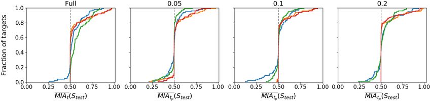
parametric test.                                                     The genotype consists of the alleles that an organism has for a
                                                                            particular characteristic.
    2. Privacy. We mount membership inference attacks [29],
       having an attacker infer whether a target record was part            SNPs and SNVs. About 99.5% of the genome is shared
       of the real data used to train the model producing the syn-          among all humans; the rest differs due to genetic variations.
       thetic dataset, as opposed to releasing the real dataset (see        Single nucleotide polymorphisms (SNPs) are the most com-
       Section 5). In the process, we also introduce a novel                mon type of genetic variation. They occur at a single position
       attack where the adversary only has partial information              in the genome and at least 1% of the population. SNPs are
       for a target individual (Section 5.2). We choose to study            usually biallelic and can be encoded by {0, 1, 2}, with 0 de-
       MIA as it is one of the most studied attacks mounted for             noting a combination of two major (i.e., common) alleles, 2
       both genomics data and machine learning, however, it has             a combination of two minor alleles, and 1 a combination of a
       never been studied in the context of synthetic genomic               major and a minor allele (which is also referred to as a het-
       data.                                                                erozygous SNP). Single nucleotide variants (SNVs) are single
                                                                            nucleotide positions in the genomic DNA at which different
Main Findings. Overall, our evaluation shows that there is                  sequence alternative exists [17].
no single approach for generating genomic synthetic data that
                                                                            Recombination Rate (RR). Recombination is the process of
performs well across the board, both in terms of utility and
                                                                            determining the frequency with which characteristics are in-
privacy. Among other things, we find that:
                                                                            herited together. The RR is the probability that a transmitted
     • A high-order correlation model specifically build for ge-            haplotype constitutes a new combination of alleles different
       nomic data (Recomb) has the best utility metrics for small           from that of either parental haplotype [14].
       datasets but does so at the cost of privacy, even against
                                                                            Genome-Wide Association Studies (GWAS). GWAS are
       weaker adversaries who only have partial information
                                                                            hypothesis-free methods for identifying associations between
       available.
                                                                            genetic regions and traits. A typical GWAS looks for common
     • The RBM model has a better performance with increasing               variants in several individuals, both with and without a trait,
       dataset sizes, both in terms of utility and privacy, as tar-         using genome-wide SNP arrays [16, 43].
       gets get stronger privacy protection when synthetic data
       is generated using a larger training set.
                                                                            2.2    Membership Inference Attacks
     • Releasing synthetic datasets does not provide robust pro-            Genomics. A well-understood privacy threat in genomics is
       tection against membership inference attacks. We find                determining whether the data of a target individual is part of
       cases where releasing the synthetic dataset sometimes of-            an aggregate genomic dataset or mixture. This is known as a
       fers better protection against membership inference at-              membership inference attack (MIA) [29, 66, 74]. The ability
       tacks. However, because of the randomness introduced                 to infer the presence of an individual’s data in a dataset consti-
       by the generative models, one cannot meaningfully pre-               tutes an inherent privacy leak whenever the dataset has some
       dict a target’s susceptibility to privacy attacks without fix-       sensitive attributes. For instance, if a mixture includes DNA
       ing the training set and quantifying the respective privacy          from patients with a specific disease, learning that a person is
       loss/gain for all targets in the set.                                part of that mixture exposes their health status.
                                                                               In general, genomic data contains extremely sensitive infor-
                                                                            mation about individuals; hence, MIAs against genomic data
2      Preliminaries                                                        prompt severe privacy threats, including denial of life/health
In this section, we introduce background information about                  insurance, revealing predisposition to diseases, ancestry, etc.
genomics, and tools used to generate synthetic data, then, we
                                                                            Machine Learning. MIAs have also been studied in the con-
present the privacy metrics and datasets used in our evaluation.
                                                                            text of machine learning to infer whether or not a target data
                                                                            point was used to train a target model. This has been done both
2.1      Genomic Primer                                                     for discriminative [11, 30, 38, 41, 51, 53, 55] and generative
Genomes and Genes. The genome represents the entirety of                    models [11, 24, 26]. Inferring training set membership might
an organism’s hereditary information. It is encoded in DNA:                 yield serious privacy violations. For instance, if a model for
each DNA strand comprises four chemical units, called nu-                   drug dose prediction is trained using data from patients with
cleotides, represented by the letters A, C, G, and T. The hu-               a certain disease, or synthetic health images are produced by
man genome consists of approximately 3 billion nucleotides                  a generative model trained on patients’ images, learning that
packaged into thread-like structures called chromosomes. The                data of a particular individual was part of the training set leaks
genome includes both the genes and the non-coding sequences                 information about that person’s health. Overall, MIAs are also
of the DNA. The former determine specific traits, character-                used as signals that access to a target model is “leaky” and can
istics, or control activity within an organism. We refer to the             be a gateway to additional attacks [24]. This is the main reason
group of genes inherited from a single parent as a haplotype.               we choose MIA as our leading privacy metric while deferring
An allele is a different variation of a gene; any individual in-            the quantification of other attacks (e.g., attribute inference or
herits two alleles for each gene, one from each of their parents.           reconstruction attacks) to future work.

                                                                        2
2.3 Privacy Gain (PG) from Synthetic Data SNPs from chromosome 13 from the following datasets:
Release
Our main privacy evaluation metric is denoted as Privacy Gain 1. CEU Population (HapMap). Samples from 117 Utah res-
(PG), first proposed in [59]. The PG quantifies the privacy idents with Northern and Western European ancestry, re-
advantage obtained by a target t, vis-à-vis an MIA adversary, leased in phase 2 of the HapMap project.
when a synthetic dataset is published instead of the real data.
2. CHB Population (HapMap). Samples from 120 Han Chi-
MIA Training (Algorithm 1). The adversary is trained as nese individuals from Beijing, China.
follows. First, we take a reference dataset (which may or may
not overlap with the real data used to generate the synthetic 3. 1,000 Genomes. Samples from 2,504 individuals from 26
dataset) and use it to generate a synthetic dataset (lines 1–6). different populations released from phase 3 of the 1000
This dataset is labeled as 0, i.e., it does not include the target Genomes project.
record (line 7). The target record is added to the dataset (line
8), and synthetic data is generated from the new dataset, which
includes the target record; this dataset is labeled as 1 (lines 3 Synthetic Data Approaches in
10-13). These models are referred to as generative shadow
models. Finally, the adversary uses the synthetic datasets to Genomics
train a classifier (line 14), which distinguishes whether or not In this section, we provide an overview of the state-of-the-art
the target was used to train a generative model. models for generating synthetic genomic data. In particular,
PG Estimation (Algorithm 2). We estimate the PG for a fixed we discuss the Recombination model presented by Samani et
target record and input dataset as follows. First, the algorithm al. [54], the RBM and GAN models proposed by Yelmen et
takes the target training set and generates ns synthetic datasets al. [71], and the WGAN model from Killoran et al. [36]. We
without the target record (lines 1–4). Then, the target record also introduce and consider two other “hybrid” models.
is added to the training set, and ns of synthetic datasets are Recombination Model (Recomb). Samani et al. [54] pro-
generated from this dataset (lines 5–9). Then, the adversary pose the use of a recombination model as an inference method
trains their attack model MIATrain (line 10). Finally, the PG for quantifying individuals’ genomic privacy. This statisti-
for a target t is computed as P Gt = 1−M IA2t (Stest ) , where cal model is based on a high-order SNV correlation that re-
M IAt (Stest ) = Si ∈Stest Pr[M IA t (Si )=1]
P
2∗ns (lines 11–12). lates linkage disequilibrium patterns to the underlying recom-
Put simply, the PG quantifies the difference between the bination rate. [54] shows how to use this method to generate
probability that an attacker correctly identifies that the target synthetic samples and perform Principal Component Analysis
record belongs to the real dataset and that that the attacker cor- (PCA). The recombination model yields a distribution closer
rectly identifies that the target record was used in training a to the real data than models using only linkage disequilibrium
generative model that outputs a synthetic dataset. and allele frequencies. The model uses a “genetic map,” which
PG Values. The PG ranges between 0, when publishing the includes the recombination rate. This is provided with the
synthetic dataset leads to the same privacy loss as publishing dataset for the HapMap datasets, but not for the 1000 genomes
the real dataset (i.e., M IAt (Stest ) = 1) and 0.5, when publish- data. For the latter, we use the scripts from [47] to generate the
ing the synthetic dataset perfectly protects the target from MIA genomic map.
(i.e., M IAt (Stest )=0). This means that P G = 0.25 when the Restricted Boltzmann Machines (RBMs). RBMs [58] are
probability of the adversary inferring whether or not a target is generative models geared to learn a probability distribution
part of the training set used to generate the synthetic dataset is over a set of inputs. RBMs are shallow, two-layer neural nets:
the same as random guessing (i.e., M IAt (Stest ) = 0.5). the first is known as the “visible” (on input) layer and the sec-
Dimensionality Reduction. To reduce the effects of high di- ond as the hidden layer. The two layers are connected via a
mensionality, the attacker first maps the synthetic data to a bipartite graph, i.e., every node in the visible layer is con-
lower feature space. This helps detect the influence of the nected to every node in the hidden one, but no two nodes in the
target record on the training dataset. We experiment with same group are connected, allowing for more efficient training
four different feature sets, as done in [59]: namely, a naive algorithms. The learning procedure consists of maximizing
feature set, which encodes the number of distinct categories the likelihood function over the visible variables of the model.
plus the most and least frequent category for each attribute, a The RBM models re-create data in an unsupervised manner
histogram, which computes the frequency counts for each at- through many forward and backward passes between the lay-
tribute, a correlation, which encodes pairwise correlations be- ers, corresponding to sampling from the learned distribution.
tween attributes, and an ensemble feature set, which combines The output of the hidden layer passes through an activation
all the previously mentioned feature sets. function, which becomes the input for the former.
As mentioned, Yelmen et al. [71] use RBMs to generate syn-
thetic genomic data. In our evaluation, we follow the same
2.4 Datasets RBM settings as [71]. More specifically, we use a ReLu acti-
Our evaluation uses data from two projects: HapMap [42] and vation function, with the visible layer having the same size as
the 1000 Genome Project [1]. More specifically, we use 1,000 the input we considered (1,000 features) and with the number
3Algorithm 1 MIATrain [59] Algorithm 2 MIAGain [59]
Input: A generative model GM(), the target record t, a reference Input: A generative model GM(), the target record t, the target train-
t
dataset R of size n, the number of synthetic test sets ns of size ing set Rout of size n, the size m of the synthetic dataset, the
m, and the number k of shadow models. number ns of synthetic test sets, a reference dataset Ra , the num-
Output: M IAt () ber k of shadow models.
1: for i = 1, · · · , k do
2: Ri ∼ Rn Output: P Gt
t
3: fi ∼ GM(Ri ) 1: fout ∼ GM(Rout )
4: for j = 1, · · · , ns do 2: for i = 1, · · · , ns do
m
5: Sjm ∼ fi 3: Si ∼ fout
6: Strain ← Strain ∪ Sjm 4: Stest ← Stest ∪ Si
t t
7: ltrain ← ltrain ∪ 0 5: Rin ← Rout ∪t
t
8: Ri0 ← Ri ∪ t 6: fin ∼ GM(Rin )
9: fi0 ∼ GM(Ri0 ) 7: for i = 1, · · · , ns do
m
10: for j = 1, · · · , ns do 8: Si ∼ fin
11: Sjm ∼ fi0 9: Stest ← Stest ∪ Si
12: Strain ← Strain ∪ Sjm 10: M IAt () ← MIATrain(GM(), t, Ra , n, m, ns , k)
P
13: ltrain ← ltrain ∪ 1 11: M IAt (Stest ) = Si ∈Stest Pr[M IAt (Si ) = 1]/2ns
14: M IAt ()←Classifier(Strain , ltrain ) 12: P Gt ← (1 − M IAt (Stest ))/2
of hidden nodes set to 100. The learning rate is set to 0.01, the Wasserstein GAN (WGAN). Killoran et al. [36] propose an
batch size to 32, and we iterate over 2,000 epochs. alternative GAN model by treating DNA sequences as a hybrid
Generative Adversarial Networks (GANs). A GAN is an between natural language and computer vision data. The se-
unsupervised deep learning model consisting of two neural quences are one-hot encoded, the GAN is based on a WGAN
networks, a generator and a discriminator, which “compete” architecture trained with a gradient penalty [22], and both
against each other. During training, the generator’s goal is to the generator and discriminator use convolutional neural net-
produce synthetic data, and the discriminator evaluates them works [37] and a residual architecture [25], which includes
against real data samples to distinguish the synthetic from the skip connections that jump over some layers. The authors also
real samples. The training objective is to learn the data dis- propose a joint method combining the GAN model with an ac-
tribution so that the data samples produced by the generator tivation maximization design [40, 57, 73] to tune the sequences
cannot be distinguished from real data by the discriminator. to have desired properties. However, we do not include the
We use the GAN approach also proposed by Yelmen et joint model in our evaluation, as we focus on a range of statis-
al. [71], mirroring their experimental settings. That is, the gen- tics instead of a single desired property.
erator model consists of an input layer with latent dimension In our evaluation, we use the WGAN model with the default
set to 600 and two hidden layers, of sizes 512 and 1,024, re- parameters from the implementation in [35]. The generator
spectively. The discriminator consists of an input layer with a consists of an input layer with a dimension of the latent space
size equal to the number of SNPs evaluated (1,000) and two set to 100, followed by a hidden layer with a size 100 times
hidden layers of sizes 512 and 256, respectively, and an output the length of the sequence (1,000), which is then reshaped to
layer of size 1. The output layer for the generator uses tanh as (length of the sequence, 100), followed by 5 resblocks. Finally,
an activation function, and the output layer for the discrimina- there is a 1-D convolutional layer followed by the output layer,
tor uses the sigmoid activation function. We compile both the which uses softmax. The discriminator has a very similar ar-
generator and discriminator using the Adam optimization and chitecture but in a different order – i.e., it starts with the input
binary cross-entropy as the loss function. layer to which the one-hot sequences are fed, that is followed
by the 1-D convolutional layer, then the 5 resblocks, followed
Recombination RBM (Rec-RBM). To overcome issues
by the reshape layer and the output layer of size 1. We per-
caused by low numbers of training samples, we propose a hy-
form 5 discriminator updates for every generator update. Both
brid approach between the Recomb and the RBM models. We
the generator and discriminator use Adam optimization, and
use the former to generate extra samples, which we then use,
their learning rates are set to 0.0001, while a gradient penalty
together with the real data samples, to train the RBM model
adjusts the loss as mentioned. We use a batch size of 64. For
with the same parameters as before. We do so to explore
more details please refer to Appendix A.
whether having more data points to train the model improves
the utility of the synthetic data.
Recombination GAN (Rec-GAN). Like Rec-RBM, we use
the Recomb model to generate extra training samples for the
4 Utility Evaluation
GAN model, using the same parameters as before. Again, This section presents a comprehensive utility evaluation of the
we want to study whether having a larger dataset available for synthetic data generated by the models introduced in Section 3.
training improves the synthetic data output’s overall utility. We look at common summary statistics used in genome-wide
4Samples
Real
Recomb
RBM
GAN
Rec-RBM
Rec-GAN
WGAN
0 200 400 600 800 1000
(a) CEU
Samples
Real
Recomb
RBM
GAN
Rec-RBM
Rec-GAN
WGAN
0 200 400 600 800 1000
(b) CHB
Samples
Real
Recomb
RBM
GAN
Rec-RBM
Rec-GAN
WGAN
0 200 400 600 800 1000
(c) 1000 Genomes
Figure 1: Major allele frequencies for synthetic data generated by the models, plotted against the real data.
association studies, aiming to assess the accuracy loss due to 4.1 Allele Statistics
the use of synthetic datasets. We choose summary statistics
Major Allele Frequency (MAF). In population genetics, the
as our main utility evaluation metrics since prior work shows
major allele frequency (MAF) is routinely used to provide
that they provide a good starting point for assessing the utility
helpful information to differentiate between common and rare
of synthetics genomic data [7, 48]. While high(er) granular-
variants in the population, as it quantifies the frequency at
ity may be required in some biomedical applications, if most
which the most common allele occurs in a given population.
generative models do not accurately replicate the high-level
We start our utility analysis by comparing MAFs in the syn-
statistics of the real data, then it is extremely unlikely they
thetic data vs. the real data.
would provide reasonable accuracy on single sequences. More
In Fig. 1, we plot the MAF at each position for the real
specifically, we analyze how well data generated by the gener-
datasets and the synthetic samples, over the CEU and CHB
ative models preserve allele frequencies, population statistics,
populations, and the 1000 Genomes dataset. For CEU/CHB
and linkage disequilibrium. We also compute the KS two-
(Fig. 1a–1b),the Recomb and WGAN replicate best the allele
sample test [27] for the goodness of fit on the most relevant
frequencies in the real data. On the other hand, GAN and Rec-
metrics in each subsection for each real dataset vs. the syn-
GAN fail to do so, and in fact, the generated samples seem
thetic data.
random. Even though not as close to the real frequencies as
Recomb, the RBM model performs better than the GAN and
Rec-GAN models. In fact, RBM further improves when com-
bined with Recomb (see Rec-RBM).
For 1000 Genomes (Fig. 1c), Recomb’s MAF distribution
5null hypothesis for Recomb, RBM and Rec-RBM.
Models CEU CHB 1000 Geno
D p-value D p-value D p-value Alternate Allele Correlation (AAC). To evaluate whether the
real and synthetic data are genetically different, in Appendix
MAF
Fig. 12, we plot the alternate allele correlation (AAC). The
Recomb 0.04 0.36 0.03 0.53 0.008 0.99 more similar the two populations are, the closer the SNPs
RBM 0.47Heterozygous
50 Population
Real
Percent calls
40
Recomb
30
RBM
20 GAN
10
Rec-RBM
Rec-GAN
0
0 100 200 300 400 500 600 700
WGAN
Sample index
(a) CEU Population
Heterozygous
50
Population
40 Real
Percent calls
30
Recomb
RBM
20 GAN
10
Rec-RBM
Rec-GAN
0
0 100 200 300 400 500 600 700
WGAN
Sample index
(b) CHB Population
Heterozygous
50 Population
Real
Percent calls
40
Recomb
30 RBM
20 GAN
Rec-RBM
10
Rec-GAN
0
0 100 200 300 400 500 600 700
WGAN
Sample index
(c) 1000 Genomes Population
Heterozygous
8
Population
7
Real
Percent calls
6
5 Recomb
4 RBM
3 Rec-RBM
2 WGAN
1
0
0 100 200 300 400 500
Sample index
(d) 1000 Genomes Population
Figure 2: Percentage of heterozygous variants in each sample in the dataset for CEU, CHB populations, and the 1000 Genomes dataset.
However, when computing the KS statistic, we find that we erozygous samples relatively similar to the real data. For this
cannot reject the null hypothesis only for those two models dataset, the only model for which we cannot reject the null
for the CEU datasets, and we reject the null hypothesis for all hypothesis is the RBM.
synthetic datasets generated from the CHB dataset. Fixation Index (FST ). Another way to assess how different
For the GAN and RBM, the percentage of heterozygous are groups of populations from each other is to use the fix-
samples decreases, suggesting that both models produce more ation index [28]. It provides a comparison of differences in
homozygous variants. Moreover, even though for the major allele frequency, with values ranging from 0 (not different) to
allele frequencies, Rec-RBM produces variants with statistics 1 (completely different/no alleles in common). In Fig. 3, we
closer to the real data, the percentage of heterozygous variants compare the FST values for the real data against the synthetic
turns out to be the lowest for both populations. By contrast, samples. For illustration purposes, we also include FST of the
Rec-GAN produces a higher percentage of heterozygous vari- real data against itself, which obviously yields FST = 0.
ants than GAN, even though the major allele frequencies are Recomb is once again the closest to the real data, which
not aligned with the original samples. With the 1000 Genomes confirms the alignment from Fig. 1 of the allele frequencies of
(Fig. 2c), the % of heterozygous samples in the real data is the synthetic recombination data with the real data. The FST
lower across all samples. Once again, and in line with previ- value for the synthetic data produced by RBM is, for both CEU
ous results, GAN and the Rec-GAN significantly deviate from and CHB populations, less than 0.10; however, the hybrid Rec-
the %s of heterozygous samples found in the real data. In fact, RBM model further reduces this value to less than 0.04, and so
in Fig. 2d, we remove the GAN and the Rec-GAN models does WGAN. For both populations, data generated by GAN
in order to take a closer look at the other models; with more and Rec-GAN has the highest FST , although, for the CHB
data samples, the samples generated yield percentages of het- population, the latter increases it, and for the CEU population
7Real vs Real tion – i.e., those alleles do not occur randomly with respect
Real vs Recomb
0.4 Real vs RBM to each other. In Genome-Wide Association Studies, LD al-
Real vs GAN lows researchers to optimize genetic studies, e.g., by prevent-
Real vs Rec-RBM
0.3 Real vs Rec-GAN ing genotyping SNPs that provide redundant information [9].
Real vs WGAN In Fig. 4, we plot the r2 value for LD based on the Rogers-
Huff method [50]. This ranges from 0 (there is no LD between
FST
0.2
the 2 SNPs) to 1 (the SNPs are in complete LD, i.e., the two
SNPs have not been separated by recombination and have the
0.1
same allele frequencies).
For CEU and CHB populations, RBM generates samples
0.0 that display a stronger LD than the real data. With more train-
CEU CHB 1000 Genomes ing samples, Rec-RBM yields a weaker LD but still stronger
Figure 3: Fixation index values (FST ) for the CEU and CHB popu- than the real data for both models. On the other side of the
lations, and the 1000 Genomes dataset. spectrum, for Rec-GAN, the LD for the synthetic data is the
weakest. For the 1000 Genomes, we find a stronger LD be-
tween the real samples than with the other two datasets. RBM
reduces it. Finally, for the 1000 genomes, Recomb, RBM, and
generates samples that are almost indistinguishable from the
Rec-RBM all have FST close to the real data. While still hav-
real data in terms of LD. The LD in the synthetic datasets gen-
ing a low FST , WGAN has a slightly higher value. Whereas,
erated by Recomb, Rec-RBM, and WGAN have lower correla-
with GAN and Rec-GAN, FST significantly deviates from the
tions than RBM, with GAN and Rec-GAN both failing to pre-
real data, even with the increased number of samples of this
serve the LD. In this case, the non-parametric KS test yields
dataset.
more surprising results for both the CEU and CHB popula-
Euclidean Genetic Distance (EGD). Since the fixation index tions. We find that we cannot reject the null hypothesis for
does not easily allow for pairwise comparisons among popu- samples generated by Recomb, GAN and WGAN. This im-
lations, in Appendix Fig. 14, we plot the Euclidean Genetic plies that, even though the GAN model does not preserve well
Distance (EGD) between the samples in each dataset. EGD is the allele frequencies or the population statistics, it manages to
routinely used as a measure of divergence between populations preserve the correlations between alleles.
and shows the number of differences, or mutations, between For the 1000 Genomes data, the only generative models that
two populations; a distance of 0 means there is no difference yields samples which cannot be rejected under the null hypoth-
in the results, i.e., there is an exact match. From Fig. 14a–14b, esis is the RBM.
where the EGD on the diagonal is 0, we observe that, for both
CEU and CHB populations, the synthetic samples generated
by GAN are closer to each other than by the other models.
4.4 Takeaways
Rec-GAN generates samples with EGD close to 0, suggesting Our utility evaluation shows that there are only a handful
that there are very few differences between them and samples of cases where generative models produce synthetic genomic
with a distance of around 30. As for the other population statis- data with high utility on popular tasks.
tics, Recomb generates samples that match the differences ob- The Recomb model, which is based on high-order SNV cor-
served in the real data the closest for both populations. For relations, generates synthetic data preserving most statistical
RBM, the samples generated have fewer differences than the properties displayed by the real data, even when few samples
real data. Perhaps more interestingly, Rec-RBM yields sam- are available. We get better utility when the genetic map is
ples with a higher divergence than the real data; this can be a included with the data rather than generated from the existing
consequence of the low percentage of heterozygous samples data. This conclusion is also supported by the fact that we can-
found in the synthetic samples generated by this model (recall not reject the null hypothesis for this model for most statistics
Fig. 2). The samples from WGAN match some of the differ- analyzed (with the exception of the percentage of heterozy-
ences observed in the real data, but the model also yields a few gous samples for the CHB).
samples with a higher divergence. With RBM, more training samples improve the quality of
Finally, for the 1000 Genomes (Fig. 14c), all samples in the the synthetic data, as evidenced by the difference between the
real data have closer EGDs between each other. In fact, the HapMap populations and the 1000 Genomes dataset.
samples generated by RBM yield a similar pattern in the EGD We also find that when few samples are available for train-
distances. Although Recomb, Rec-RBM, and WGAN do too, ing, the hybrid Rec-RBM model approach helps improve the
they exhibit a lower distance, on average, between samples. As quality of samples compared to just RBM, but the samples are
for CEU/CHB populations, GAN and Rec-GAN models fail to not as close to the real data as for Recomb. This is clear from
capture the differences between samples. the utility of the synthetic data on the two smaller HapMap
datasets. For the 1000 genomes, it is not surprising that Rec-
RBM’s performance is worse than RBM since Recomb does
4.3 Linkage Disequilibrium (LD) Analysis not generate as “useful” samples as for the other two datasets.
Linkage disequilibrium (LD) captures the non-random associ- Finally, the GAN and the Rec-GAN models generate sam-
ation of alleles at two or more positions in a general popula- ples with the lowest utility, regardless of the number of sam-
8(a) CEU
(b) CHB
(c) 1000 Genomes
Figure 4: Pairwise Linkage Disequilibrium for Real vs. Synthetic Samples.
ples available for training. However, even though the allele thetic datasets, with a split of 50 sets generated from a training
and population statistics are now well preserved, our non- set including the target and 50 sets generated without. Finally,
parametric test showcases that the correlations between alleles we report the PG for each test and each target as the average
are preserved for the LD. In contrast to the other GAN models PG across all synthetic datasets tested.
studied, the data generated by WGAN preserves most statisti-
cal properties of the real data.
Overall, our analysis exposes the limitations, in terms of sta-
5.1 Privacy Gain Under Membership
tistical utility, of using generative machine learning models to Inference Attack
produce synthetic genomic data. Threat Model. We assume that the adversary has access to the
target, to the synthetic datasets, as well as public datasets with
similar distribution to the original data (which may or may not
5 Privacy Evaluation include the target) for training his shadow models. The goal
Next, we quantify the privacy provided by synthetic data by of the adversary is to identify whether the target sequence was
evaluating its vulnerability to Membership Inference Attacks used for training the model that generated the synthetic dataset.
(MIAs). More precisely, we compute the Privacy Gain, PG, This could lead to the leakage of additional information about
obtained by releasing a synthetic dataset instead of the real the target, as for example if a synthetic dataset of cancer pa-
data (see Section 2.3). Recall that if the synthetic data does not tients is released and the adversary can identify that the target
hide nor give any additional information to an MIA attacker, is part of the training set, it would lead to exposing the cancer
P Gt , for a target record t, should have a value of around 0.25. status of the target.
We present experiments for both a “standard” MIA and a We use three adversarial classifiers: K-Nearest Neighbor
novel attack, which we denote as MIA with partial informa- (KNN), Logistic Regression (LogReg), and Random Forest
tion. The latter essentially assumes that the adversary only has (RandForest). We use four feature sets, as described in Sec-
access to partial data from the target sequence. We exclude tion 2.3: Naive ( FNaive ), Histogram ( FHist ), Correlations
GAN and Rec-GAN from the evaluation since they yield poor ( FCorr ), and an Ensemble feature set ( FEns ).
utility performance, so there is not really any point in evaluat- 5.1.1 HapMap Populations
ing their privacy.
Throughout our evaluation, we randomly choose 10 targets In Fig. 5, we report the PG value for targets randomly chosen
from each dataset across 10 test runs. In each run, we fix the from the two HapMap populations.
target and sample a new training cohort. We train the attack KNN. For CEU, using KNN (Fig. 5a, left), we find that over
classifier using 5 shadow models, using 100 synthetic training 74% of the targets in the synthetic dataset generated by Re-
sets for each of them. We then compute the PG on 100 syn- comb have a PG lower than the random baseline (0.25) for
9KNN LogReg RandForest
0.5
0.4
0.3
PGt
0.2
0.1
0.0
Recomb RBM Rec-RBM WGAN Recomb RBM Rec-RBM WGAN Recomb RBM Rec-RBM WGAN
(a) CEU Population
KNN LogReg RandForest
0.5
0.4
0.3
PGt
0.2
0.1
0.0
Recomb RBM Rec-RBM WGAN Recomb RBM Rec-RBM WGAN Recomb RBM Rec-RBM WGAN
(b) CHB Population
Figure 5: Privacy Gain (PG) of different models over the two HapMap populations.
the Ensemble, Correlations, and Histogram feature sets. With 0.25. Moreover, for the Rec-RBM and WGAN-generated data,
RBM, there are between 84% and 88% of the targets, depend- no target consistently has a lower PG than the random guess
ing on the feature set, that have a PG of 0.25; in other words, baseline across all test runs.
for these targets, the adversary’s probability of inferring their For CHB (Fig. 5b, middle), with synthetic data generated by
presence in the training set is the same as random guessing. Recomb, the average PG is below the random baseline (0.25)
However, between 10% and 15% of the targets have no PG for 99% of the targets in the Histogram feature set, 97% for
at all, whereas there are between 1% and 4% of the targets, Correlations, and 96% for Ensemble. For RBM, 79% of the
depending on the feature set, for which the synthetic data per- targets in the Histogram feature set have a PG below 0.25. Un-
fectly protects the target from MIA (PG=0.5). With Rec-RBM, der the Ensemble feature set, 84% of the targets have PG below
at least 59% of the targets have a PG of 0.25 under the four fea- 0.25. For synthetic data generated by Rec-RBM, we find that
ture sets. With WGAN, at least 48% of the targets have a PG 54% of the targets from the Histogram and Ensemble feature
of 0.25, depending on the feature set. sets have PG lower than 0.25, and 46% have PG over 0.25.
For the CHB population (Fig. 5b, left), we find that over For the Naive and Correlations feature sets, respectively, 45%
60% of the targets generated by the Recomb, with all features, and 47% of the targets have PG lower than the random guess
have PG below the random guess baseline. With RBM, be- baseline. For WGAN-generated data, the Correlations feature
tween 89% and 97% of targets have PG of exactly 0.25 across set yields most targets (55%) with PG0.5 0.5
0.4 0.4
0.3 0.3
PGt
PGt
0.2 0.2
0.1 0.1
0.0 0.0
RandForest LogReg KNN RandForest LogReg KNN
(a) Random Target (b) Outlier target
Figure 6: Privacy Gain (PG) of RBM over the 1000 Genomes dataset.
have a PG of 0.25, meaning that those targets are protected gain than in the random target case. For the Naive feature set,
from MIA. For the synthetic samples generated by Rec-RBM, PG is below the random baseline in only 3 of the test runs.
54% of the targets from the Histogram and Ensemble feature For the Correlations and Histogram feature sets, all test runs
sets and 47 and 45% of the targets from the Correlations and yield PG of 0.25 or above. With LogReg, 4 out of 10 of the
Naive, respectively, have PG lower than 0.25. Finally, for the test runs for the Naive, Histogram, and Correlations feature
WGAN, we find that between 44% and 53% of the targets have sets yield PG below 0.25. For Ensemble, this happens for 6
PG>0.25 across all four feature sets. To give a better idea of test runs. Finally, with KNN, across all feature sets, PG for all
different trade-offs between utility and privacy, we also plot test runs is 0.25, i.e., the synthetic data does not disclose any
the PG vs. the FST (see Section 4.2) for all the models pre- membership information regarding the outlier.
sented in Appendix D. While there are differences across classifiers/feature sets,
5.1.2 1000 Genomes Population the PG is centered around 0.25 for all test runs in the outlier
target setting. This evident from Figure 6b, which implies that,
For this dataset, we focus our analysis on the RBM model, as across all test runs, the accuracy of the MIA is not much better
it generated synthetic data closest to the real data across all than random guessing.
utility metrics evaluated.
Random Target. In Figure 6a, we plot the PG for the synthetic 5.1.3 Takeaways
data generated by RBM for randomly chosen targets. With the The different combinations of datasets, attack classifiers, and
RandForest MIA classifier, we observe that 56%, 75%, 92%, feature sets yield varied results with respect to privacy. This
and 50% of the targets have PG higher than the random guess is due to two main reasons: first, not all classifiers have the
baseline (PG≥0.25) for, respectively, Naive, Histogram, Cor- same accuracy on tasks for the same dataset, as shown in pre-
relations, and Ensemble feature sets. The high percentage of vious work [3]. Second, the features that the generative model
targets that have a PG≥0.25 for the Correlations suggests that preserves after training will “reflect” in the synthetic data;
the impact of a single target in the training dataset of the RBM thus, this will impact the PG based on the feature extraction
on the correlations of the synthetic dataset is minimal. method. On the HapMap populations, while the utility experi-
Then, with the LogReg classifier, we find a high variation ments show that Recomb-generated synthetic data is “closest”
in PG, similar to the HapMap populations in the case of Rec- to the real data, it does so with a significant privacy loss. The
RBM. Under the Naive feature set, half of the targets have PG RBM-generated synthetic data is the most vulnerable under
gain below the random guess baseline. Similarly, 43%, 45%, the LogReg classifier, with at least 70% of the targets across
and 43% of targets have a PG lower than 0.25 for, respectively, both populations and all feature sets having PG below the ran-
the Correlations, Histogram, and Ensemble feature sets. Fi- dom guess baseline. This suggests that, with few data samples
nally, for the KNN classifier, over 94% of the targets have a available for training, the RBM model is likely to overfit and
PG of 0.25 across all feature sets. is thus susceptible to MIAs.
Outlier Target. To better understand whether or not, with For Rec-RBM and WGAN, the attacker cannot reliably pre-
more training data, a target’s signal in the synthetic dataset dict membership, i.e., extra samples from the Recomb model
is diluted, we also test an “extreme” outlier case. That is, we in the training of the Rec-RBM dilute the target’s signal in the
craft an outlier target that has only minor alleles at all posi- training data. However, for both models, we still find combi-
tions. While we are aware that this case would be sporadic in nations of targets and training sets for the attack classifier for
a real-world scenario, our goal is to observe whether and how which PG is significantly lower than the random guess base-
much this impacts PG. To this end, in Figure 6b, we plot the line; i.e., the synthetic data will still expose membership infor-
PG of this outlier case across 10 test runs. mation about the respective targets. On the 1000 Genomes, PG
With RandForest, we find that PG is below 0.25 for 8 of the values have a higher variation overall when the target is chosen
10 test runs under the Ensemble feature set. In fact, this is the randomly from the dataset than for the two smaller HapMap
only combination between attack classifier and feature set for datasets. The results for RBM confirm our hypothesis that the
which a greater percentage of the targets have a lower privacy target’s influence is diluted within larger datasets. Once again,
11this does not mean that MIAs are not possible for Rec-RBM target is part of the real dataset versus the target being part of
and WGAN; it depends on the combination of the target, train- the training set used to generate the synthetic dataset.
ing set, attack classifier, and feature set. As a result, PG now ranges between -0.5 and 0.5, where
However, with an “extreme” outlier (i.e., a target with minor 0.5 means that having the real dataset R and the partial in-
alleles at all positions), the synthetic data generated by RBM formation t0 about the target allows the adversary to infer the
does not have a big impact on PG. In this case, the PG is actu- membership of t in R, while the synthetic dataset reduces
ally close to the random guess baseline across all test runs. the adversary’s chance of success (i.e. M IAtp (Rt ) = 1 and
We find that targets get very different levels of privacy pro- M IAtp (Stest ) = 0). A negative PG value means that publish-
tection, based on the combination of target and training set ing the synthetic data, instead of the real data, improves the
used to generate the synthetic data. For a privacy mechanism adversary’s chance to correctly infer membership of the tar-
to provide good privacy protection, it needs to be predictable, get t (i.e. M IAtp (Rt ) < M IAtp (Stest )). If publishing the
i.e., all targets should have a privacy gain above the random synthetic data does not increase nor decrease the adversary’s
guess baseline, which our evaluation shows it is not the case inference powers, we should have PG=0 (i.e. M IAtp (Rt ) =
for the data generated by the models we have evaluated. M IAtp (Stest )).
Experiments. From the experiments presented in Section 5.1,
5.2 Privacy Gain under Membership Inference we find that the attack classifier that yields the lowest PG is
Attack with Partial Information Logistic Regression; thus, we only experiment with that one
Next, we introduce a novel attack, which we denote as MIA to ease presentation. In the following, we present the results
with Partial Information (MIA-PI). Basically, we only give the of the MIA-PI experiments for the CEU population, focusing
attacker access to a fraction of SNVs from the target sequence, on the Recomb and RBM models (as mentioned, with a Lo-
chosen at random. The attacker then uses the Recombination gReg attack classifier). We do so as these two models yield the
model from [54] as an inference method to predict the rest of lowest PG in Section 5.1.
the sequence. Compared to the previous attack, the adversary Recomb. In Figure 7, we plot the Cumulative Distribution
trains their (attack) classifier using the sequence inferred from Function (CDF) of the accuracy of the attack for Recomb when
the partial data. Thus, the PG formula also needs to be adjusted the adversary has access to the full sequence vs. partial infor-
to account for how likely an adversary is to identify a target mation, specifically, a ratio of 0.05, 0.1, and 0.2 of the total
from partial information. SNVs from the target sequence. Interestingly, even when only
Threat Model. We assume that, similar to the MIA attack, the 0.05 of the target SNVs are available to the attacker, for 90%
adversary has access to the synthetic dataset, as well as public and 91% of the targets from the Histogram and respectively
datasets with similar distribution to the original data (which Ensemble feature sets, the attacker’s accuracy is still above the
may or may not include the target) for training his shadow random guess baseline (50% accuracy). Our intuition is that
models. In contrast with the previous MIA, the adversary does many targets are vulnerable to the attack, even with little par-
not obtain access to the full sequence of the target, but only to tial information, since we use the Recomb model not only for
a percentage of the SNPs from the target sequence (as for ex- the attack but also as an inference method to predict the rest of
ample, the victim undertakes some specific genomic tests and the sequence.
the adversary learns that information about the victim from To explore how much of the MIA-PI vulnerability is due to
the outcome of those tests), as well as public knowledge about the release of synthetic datasets, and not only by how much
genomic data. The goal of the adversary is to identify if the information the attacker has available, in Figure 8, we plot the
partial target sequence was part of the training set which gen- CDF of the PG with MIA-PI. In line with the accuracy results,
erated the synthetic data. we find that the PG is greater than 0 for at least 88% of the
targets for all ratios of partial information tested in the case
PG for MIA-PI. Assuming the attacker has partial informa- of the Correlations feature set. However, for the other three
tion t0 as a fraction of the SNVs from t, they first use the Re- feature sets, releasing the synthetic dataset instead of the real
comb model, as an inference algorithm, to predict the rest of data decreases the privacy gain (i.e., PGFigure 7: Accuracy of the Membership Inference Attack with access Figure 9: Accuracy of the Membership Inference Attack with access
to full and partial information (0.05, 0.1, and 0.2 ratio) for Recomb. to full and partial information (0.05, 0.1, and 0.2 ratio) for RBM.
1.0 0.05 0.1 0.2 0.05 0.1 0.2
1.0
Fraction of targets
0.8
Fraction of targets
0.8
0.6 0.6
0.4 0.4
0.2 0.2
0.0 0.0
0.50 0.25 0.00 0.25 0.50 0.50 0.25 0.00 0.25 0.50 0.50 0.25 0.00 0.25 0.50 0.50 0.25 0.00 0.25 0.50 0.50 0.25 0.00 0.25 0.50 0.50 0.25 0.00 0.25 0.50
PGt PGt PGt PGt PGt PGt
Figure 8: Privacy Gain (PG) for synthetic samples from Recomb. Figure 10: Privacy Gain (PG) for synthetic samples generated by
RBM.
to the full sequence.
RBM. In Figure 9, we plot the CDF for the accuracy of the tion of an autoencoder with a GAN model, called medGAN,
attack for the RBM model for both full and partial informa- to generate high-dimensional multi-label discrete data. ADS-
tion about the target record available to the attacker. Across all GAN [72] uses a quantifiable definition for “identifiability”
feature sets, there is an increase in the accuracy of the attack combined with the discriminator’s loss to minimize the prob-
with more information available to the attacker, as is expected. ability of patient’s re-identification, while CorGAN [61] com-
We also look at CDF for the PG in the case of partial informa- bines convolutional GANs and convolutional autoencoders to
tion available to the attacker in Figure 10. Once again, under capture the correlations between adjacent medical features.
the Naive feature set, increasing the partial information avail- Biswal et al. [8] use variational autoencoder to synthesize se-
able to the attacker negatively correlates with the percentage quences of discrete EHR encounters and encounter features.
of targets with a negative PG. Under all other feature sets, for Other initiatives focus on synthetic data modeled on pri-
most targets, releasing the synthetic dataset instead of the real mary care data [45, 63, 64, 68]. Researchers have also ex-
data yields a positive PG, meaning that releasing the synthetic plored generating synthetic health patient data to detect cancer
dataset instead of the real dataset improves the PG. and other diseases, e.g., RDP-CGAN [62] combines convo-
lutional GANs and convolutional autoencoders, both trained
Takeaways. We find that not even decreasing the attacker’s with Rényi differential privacy [39].
power by only giving him partial information from the tar-
Specific to genomes is the work presented in Section 3 [36,
get sequence mitigates privacy for the Recomb-generated syn-
54, 71], which we have evaluated in terms of their utility–
thetic data. This is likely because, using the Recomb model
privacy tradeoffs.
as both generative and inference model, the adversary’s power
is increased since the feature set extracted from the synthetic Privacy in Genomics. Researchers have focused on study-
data will be closer to the feature set for the predicted target. ing and mitigating privacy risks in genomics. One of the first
However, in this case, for RBM, we see an increase in the attacks on genomic data is the Membership Inference Attack
privacy gained by releasing synthetic data instead of real data. proposed by Homer et al. [29], showing that an adversary can
This implies that, even if the RBM is likely to overfit when few infer the presence of an individual’s genotype within a com-
samples are available for training, it does so on the predicted plex DNA mixture. This attack has been improved by Wang
sequence of the target rather than on the full sequence and thus et al. [66] using correlation statistics of a few hundred SNPs.
decreases the accuracy of the MIA. Then, Im et al. [32] show that the summary information from
Overall, not even with partial data from the target sequence, genome-wide association studies, such as regression coeffi-
we obtain privacy gain values constantly better than random cients, can also reveal an individual’s participation within the
guessing, which, as mentioned before, indicates that synthetic respective study. Membership inference has also been shown
data is not really a reliable privacy defense. possible in the context of the Beacon network [49, 56, 65], a
federated service that answers queries of the form “does your
data have a specific nucleotide at a specific genomic coordi-
nate?”.
6 Related Work Chen et al. [12] study the effects of differential privacy pro-
In this section, we review related work on synthetic data, ge- tection against membership inference attack on machine learn-
nomic privacy, and MIAs against machine learning models. ing for genomic data. However, their study is focused on
Synthetic Data Initiatives. In recent years, researchers privacy leakage via providing access to trained classification
have focused on generating synthetic electronic health records models, whereas we study the privacy leakage from sharing
(EHR), aiming to facilitate research in and adoption of ma- synthetic datasets.
chine learning in medicine. Choi et al. [13] use a combina- MIAs against Machine Learning Models. MIAs have long
13been studied in the context of machine learning. Shokri et dataset; also, we measured a decrease in the number of targets
al. [55] present the first attack against discriminative models, exposed to membership inference.
aiming to identify whether a data record was used in train- We also introduced a new “MIA with partial information,”
ing, using an approach based on shadow models. Hui et which shed light on the fact that not even decreasing the ad-
al. [30] also propose an attack against discriminative models, versary’s power by limiting their knowledge of the target to
which probes the target model and infers membership directly partial information fully mitigates the privacy loss. Finally,
from the probes instead of shadow models. Hayes et al. [24] our modular evaluation framework paves the way for practi-
present the first MIA against generative models like GANs; tioners, scientists, and researchers to easily build on our work
they use a discriminator to output the data with the highest and assess the risks of deploying synthetic genomic data in the
confidence values as the original training data. Hilprecht et wild, for a wide range of applications, and serve as a bench-
al. [26] study MIAs against both GANs and Variational Au- mark for techniques proposed in the future.
toEncoders (VAEs), while Chen et al. [11] propose a generic Limitations & Future Work. Our evaluation focuses on ex-
MIA model against GANs. isting generative methods for synthetic genomic data; thus, we
Stadler et al. [59] recently evaluate MIAs in the context of have not engaged in fine-tuning the (hyper-)parameters of the
synthetic data and show that even access to a single synthetic models evaluated. Moreover, one might argue that the tech-
dataset output by the target model can lead to privacy leak- niques we evaluate were not designed with privacy in mind,
age. We re-use their framework for quantifying the privacy unlike previous work on differentially private generative mod-
gain when a synthetic dataset is released instead of the real els for images or clinical data [2, 6, 10]. That is, it is not en-
dataset. However, not only do we do so for a specific con- tirely surprising that they yield small privacy gains. However,
text (namely, genomics), but we also measure utility (while to the best of our knowledge, no differentially private genera-
they only study privacy). In fact, there are several distinguish- tive model has been proposed for genomic data, which is the
ing characteristics between “generic” synthetic data and ge- focus of our study.
nomic data, which makes the evaluation significantly differ- In fact, prior work has shown that, for precision medicine
ent, if not harder; paramount among these is the fact that all applications, the high dimensionality of the data tends to be
features found in genomic sequences are correlated with each a major limitation, resulting in poor utility for differentially
other, unlike with generic datasets. Finally, we introduce and private mechanisms [5, 20, 34, 69, 70]. Differentially private
measure a novel attack whereby the attacker only has access to techniques for GWAS are also known to yield poor accuracy
partial genomic information about the target. as the number of features is large, relative to the number of
patients in a study [33]. Nonetheless, we plan to experiment
with the possible adaptation of differentially private models to
7 Conclusion genomic data and evaluate them in future work.
This paper presented an in-depth measurement of state-of-the- Finally, future work should search for, and experiment with,
art methods to generate synthetic genomic data. We did so vis- genomics use cases that have more data points, possibly rely-
à-vis their utility, with respect to several common analytical ing on further collaborations with biomedical researchers. We
tasks performed by researchers and the privacy protection they also intend to extend our privacy evaluation to understand how
provide compared to releasing real data. much the privacy loss stemming from releasing (synthetic)
datasets affects the relatives of those included in the training
High-quality synthetic data must accurately capture the re-
set of the corresponding generative models [31, 60].
lations between data points; however, this can enable attackers
to infer sensitive information about the training data used to Acknowledgments. This work was supported by a Google
generate the synthetic data. This was illustrated by the perfor- Faculty Award on “Enabling Progress in Genomic Research
mance of the Recomb model on the HapMap datasets: while via Privacy Preserving Data Sharing.”
it achieves the best utility, it does so at the cost of significantly
reducing privacy.
References
Discussion. Overall, we found that there is no single method
that outperforms the others for all metrics and all datasets. [1] 1000 Genomes Project Consortium. A global reference for hu-
While this is perhaps not surprising, we are the first to present man genetic variation. Nature, 526(7571), 2015.
a systematic, re-usable methodology to analyze all kinds of [2] G. Acs, L. Melis, C. Castelluccia, and E. De Cristofaro.
Differentially private mixture of generative neural networks.
methods to generate synthetic genomic data. For instance, this
IEEE Transactions on Knowledge and Data Engineering,
allows us to be the first to show that, unlike what previously
31(6):1109–1121, 2018.
suggested in previous work, models based on a simple GAN
[3] D. R. Amancio, C. H. Comin, D. Casanova, G. Travieso, O. M.
architecture (i.e., GAN and Rec-GAN) are not a good fit for Bruno, F. A. Rodrigues, and L. da Fontoura Costa. A systematic
genomic data. In fact, these provide low (the lowest) utility comparison of supervised classifiers. PloS one, 9(4), 2014.
across the board. Our methodology also allowed us to shed [4] E. Ayday, E. De Cristofaro, J.-P. Hubaux, and G. Tsudik. Whole
light on the influence of the size of the training dataset, es- genome sequencing: Revolutionary medicine or privacy night-
pecially in the case of generative models. For example, util- mare? Computer, 48(2), 2015.
ity improves wit more samples in the hybrid Rec-RBM for the [5] C.-A. Azencott. Machine learning and genomics: precision
smaller HapMap datasets, and the RBM for the 1000 Genomes medicine versus patient privacy. Philosophical Transactions of
14You can also read