A connectome and analysis of the adult Drosophila central brain - eLife
←
→
Page content transcription
If your browser does not render page correctly, please read the page content below
RESEARCH ARTICLE

                                    A connectome and analysis of the adult
                                    Drosophila central brain
                                    Louis K Scheffer1†*, C Shan Xu1†, Michal Januszewski2†, Zhiyuan Lu1,3†,
                                    Shin-ya Takemura1†, Kenneth J Hayworth1†, Gary B Huang1†,
                                    Kazunori Shinomiya1†, Jeremy Maitlin-Shepard4, Stuart Berg1, Jody Clements1,
                                    Philip M Hubbard1, William T Katz1, Lowell Umayam1, Ting Zhao1,
                                    David Ackerman1, Tim Blakely2, John Bogovic1, Tom Dolafi1,
                                    Dagmar Kainmueller1‡, Takashi Kawase1, Khaled A Khairy1§, Laramie Leavitt2,
                                    Peter H Li2, Larry Lindsey2, Nicole Neubarth1#, Donald J Olbris1, Hideo Otsuna1,
                                    Eric T Trautman1, Masayoshi Ito1,5, Alexander S Bates6, Jens Goldammer1,7,
                                    Tanya Wolff1, Robert Svirskas1, Philipp Schlegel6, Erika Neace1,
                                    Christopher J Knecht1, Chelsea X Alvarado1, Dennis A Bailey1,
                                    Samantha Ballinger1, Jolanta A Borycz3, Brandon S Canino1, Natasha Cheatham1,
                                    Michael Cook1, Marisa Dreher1, Octave Duclos1, Bryon Eubanks1, Kelli Fairbanks1,
                                    Samantha Finley1, Nora Forknall1, Audrey Francis1, Gary Patrick Hopkins1,
                                    Emily M Joyce1, SungJin Kim1, Nicole A Kirk1, Julie Kovalyak1, Shirley A Lauchie1,
                                    Alanna Lohff1, Charli Maldonado1, Emily A Manley1, Sari McLin3,
*For correspondence:                Caroline Mooney1, Miatta Ndama1, Omotara Ogundeyi1, Nneoma Okeoma1,
schefferl@janelia.hhmi.org (LKS);   Christopher Ordish1, Nicholas Padilla1, Christopher M Patrick1, Tyler Paterson1,
plazas@janelia.hhmi.org (SMP)
                                    Elliott E Phillips1, Emily M Phillips1, Neha Rampally1, Caitlin Ribeiro1,
†
 These authors contributed          Madelaine K Robertson3, Jon Thomson Rymer1, Sean M Ryan1, Megan Sammons1,
equally to this work                Anne K Scott1, Ashley L Scott1, Aya Shinomiya1, Claire Smith1, Kelsey Smith1,
Present address: ‡Max               Natalie L Smith1, Margaret A Sobeski1, Alia Suleiman1, Jackie Swift1,
Delbrueck Centre for                Satoko Takemura1, Iris Talebi1, Dorota Tarnogorska3, Emily Tenshaw1,
Developmental Medicine, Berlin,     Temour Tokhi1, John J Walsh1, Tansy Yang1, Jane Anne Horne3, Feng Li1,
Germany; §Department of             Ruchi Parekh1, Patricia K Rivlin1, Vivek Jayaraman1, Marta Costa8,
Developmental Neurobiology,         Gregory SXE Jefferis6,8, Kei Ito1,5,7, Stephan Saalfeld1, Reed George1,
St. Jude Children’s Research
                                    Ian A Meinertzhagen1,3, Gerald M Rubin1, Harald F Hess1, Viren Jain4,
Hospital, Memphis, United
States; #Two Six Labs, Arlington,
                                    Stephen M Plaza1*
United States                       1
                                      Janelia Research Campus, Howard Hughes Medical Institute, Ashburn, United
Competing interest: See
                                    States; 2Google Research, Mountain View, United States; 3Life Sciences Centre,
page 51
                                    Dalhousie University, Halifax, Canada; 4Google Research, Google LLC, Zurich,
Funding: See page 52
                                    Switzerland; 5Institute for Quantitative Biosciences, University of Tokyo, Tokyo,
Received: 31 March 2020             Japan; 6MRC Laboratory of Molecular Biology, Cambridge, United States; 7Institute
Accepted: 01 September 2020         of Zoology, Biocenter Cologne, University of Cologne, Cologne, Germany;
Published: 07 September 2020        8
                                      Department of Zoology, University of Cambridge, Cambridge, United Kingdom
Reviewing editor: Eve Marder,
Brandeis University, United
States
   Copyright Scheffer et al. This   Abstract The neural circuits responsible for animal behavior remain largely unknown. We
article is distributed under the    summarize new methods and present the circuitry of a large fraction of the brain of the fruit fly
terms of the Creative Commons       Drosophila melanogaster. Improved methods include new procedures to prepare, image, align,
Attribution License, which          segment, find synapses in, and proofread such large data sets. We define cell types, refine
permits unrestricted use and        computational compartments, and provide an exhaustive atlas of cell examples and types, many of
redistribution provided that the    them novel. We provide detailed circuits consisting of neurons and their chemical synapses for
original author and source are      most of the central brain. We make the data public and simplify access, reducing the effort needed
credited.

Scheffer, Xu, Januszewski, et al. eLife 2020;9:e57443. DOI: https://doi.org/10.7554/eLife.57443                                 1 of 83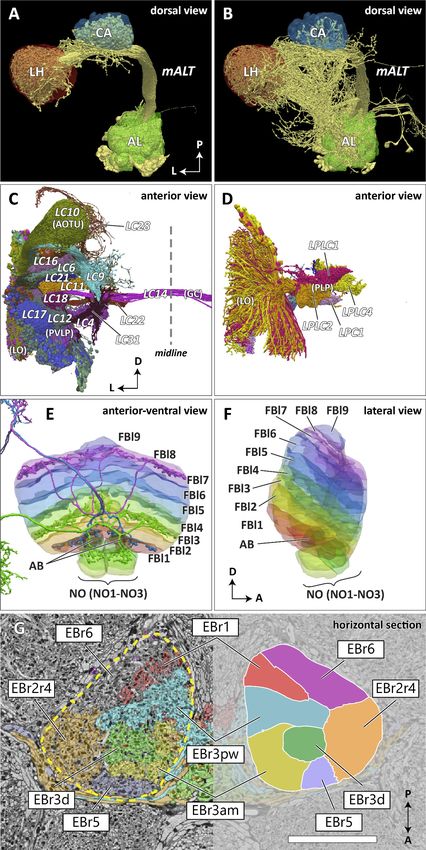
Research article                                                                       Computational and Systems Biology Neuroscience

                                    eLife digest Animal brains of all sizes, from the smallest to the largest, work in broadly similar
                                    ways. Studying the brain of any one animal in depth can thus reveal the general principles behind
                                    the workings of all brains. The fruit fly Drosophila is a popular choice for such research. With about
                                    100,000 neurons – compared to some 86 billion in humans – the fly brain is small enough to study at
                                    the level of individual cells. But it nevertheless supports a range of complex behaviors, including
                                    navigation, courtship and learning.
                                       Thanks to decades of research, scientists now have a good understanding of which parts of the
                                    fruit fly brain support particular behaviors. But exactly how they do this is often unclear. This is
                                    because previous studies showing the connections between cells only covered small areas of the
                                    brain. This is like trying to understand a novel when all you can see is a few isolated paragraphs.
                                       To solve this problem, Scheffer, Xu, Januszewski, Lu, Takemura, Hayworth, Huang, Shinomiya
                                    et al. prepared the first complete map of the entire central region of the fruit fly brain. The central
                                    brain consists of approximately 25,000 neurons and around 20 million connections. To prepare the
                                    map – or connectome – the brain was cut into very thin 8nm slices and photographed with an
                                    electron microscope. A three-dimensional map of the neurons and connections in the brain was then
                                    reconstructed from these images using machine learning algorithms. Finally, Scheffer et al. used the
                                    new connectome to obtain further insights into the circuits that support specific fruit fly behaviors.
                                       The central brain connectome is freely available online for anyone to access. When used in
                                    combination with existing methods, the map will make it easier to understand how the fly brain
                                    works, and how and why it can fail to work correctly. Many of these findings will likely apply to larger
                                    brains, including our own. In the long run, studying the fly connectome may therefore lead to a
                                    better understanding of the human brain and its disorders. Performing a similar analysis on the brain
                                    of a small mammal, by scaling up the methods here, will be a likely next step along this path.

                                    to answer circuit questions, and provide procedures linking the neurons defined by our analysis
                                    with genetic reagents. Biologically, we examine distributions of connection strengths, neural motifs
                                    on different scales, electrical consequences of compartmentalization, and evidence that maximizing
                                    packing density is an important criterion in the evolution of the fly’s brain.

                                    Introduction
                                    The connectome we present is a dense reconstruction of a portion of the central brain (referred to
                                    here as the hemibrain) of the fruit fly, Drosophila melanogaster, as shown in Figure 1. This region
                                    was chosen since it contains all the circuits of the central brain (assuming bilateral symmetry), and in
                                    particular contains circuits critical to unlocking mysteries involving associative learning in the mush-
                                    room body, navigation and sleep in the central complex, and circadian rhythms among clock circuits.
                                    The largest dense reconstruction to date, it contains around 25,000 neurons, most of which were rig-
                                    orously clustered and named, with about 20 million chemical synapses between them, plus portions
                                    of many other neurons truncated by the boundary of the data set (details in Figure 1). Each neuron
                                    is documented at many levels - the detailed voxels that constitute it, a skeleton with segment diame-
                                    ters, its synaptic partners and the location of most of their synapses.
                                        Producing this data set required advances in sample preparation, imaging, image alignment,
                                    machine segmentation of cells, synapse detection, data storage, proofreading software, and proto-
                                    cols to arbitrate each decision. A number of new tests for estimating the completeness and accuracy
                                    were required and therefore developed, in order to verify the correctness of the connectome.
                                        These data describe whole-brain properties and circuits, as well as contain new methods to clas-
                                    sify cell types based on connectivity. Computational compartments are now more carefully defined,
                                    we conclusively identify synaptic circuits, and each neuron is annotated by name and putative cell
                                    type, making this the first complete census of neuropils, tracts, cells, and connections in this portion
                                    of the brain. We compare the statistics and structure of different brain regions, and for the brain as
                                    a whole, without the confounds introduced by studying different circuitry in different animals.

Scheffer, Xu, Januszewski, et al. eLife 2020;9:e57443. DOI: https://doi.org/10.7554/eLife.57443                                          2 of 83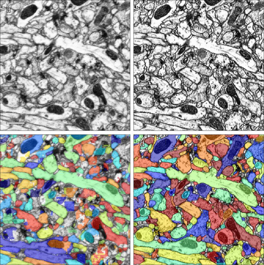
Research article                                                                         Computational and Systems Biology Neuroscience

                                         All data are publicly available through web interfaces. This includes a browser interface, NeuPrint
                                     (Clements et al., 2020), designed so that any interested user can query the hemibrain connectome
                                     even without specific training. NeuPrint can query the connectivity, partners, connection strengths
                                     and morphologies of all specified neurons, thus making identification of upstream and downstream
                                     partners both orders of magnitude easier, and significantly more confident, compared to existing
                                     genetic methods. In addition, for those who are willing to program, the full data set - the gray scale
                                     voxels, the segmentation and proofreading results, skeletons, and graph model of connectivity, are
                                     also available through publicly accessible application program interfaces (APIs).
                                         This effort differs from previous EM reconstructions in its social and collaborative aspects. Previ-
                                     ous reconstructions were either dense in much smaller EM volumes (such as Meinertzhagen and
                                     O’Neil, 1991; Helmstaedter et al., 2013; Takemura et al., 2017) or sparse in larger volumes (such
                                     as Eichler et al., 2017 or Zheng et al., 2018). All have concentrated on the reconstruction of spe-
                                     cific circuits to answer specific questions. When the same EM volume is used for many such efforts,
                                     as has occurred in the Drosophila larva and the full adult fly brain, this leads to an overall reconstruc-
                                     tion that is the union of many individual efforts (Saalfeld et al., 2009). The result is inconsistent

Figure 1. The hemibrain and some basic statistics. The highlighted area shows the portion of the central brain that was imaged and reconstructed,
superimposed on a grayscale representation of the entire Drosophila brain. For the table, a neuron is traced if all its main branches within the volume
are reconstructed. A neuron is considered uncropped if most arbors (though perhaps not the soma) are contained in the volume. Others are
considered cropped. Note: (1) our definition of cropped is somewhat subjective; (2) the usefulness of a cropped neuron depends on the application;
and (3) some small fragments are known to be distinct neurons. For simplicity, we will often state that the hemibrain contains » 25K neurons.

Scheffer, Xu, Januszewski, et al. eLife 2020;9:e57443. DOI: https://doi.org/10.7554/eLife.57443                                                   3 of 83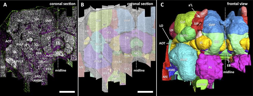
Research article                                                                       Computational and Systems Biology Neuroscience

                                    coverage of the brain, with some regions well reconstructed and others missing entirely. In contrast,
                                    here we have analyzed the entire volume, not just the subsets of interest to specific groups of
                                    researchers with the expertise to tackle EM reconstruction. We are making these data available with-
                                    out restriction, with only the requirement to cite the source. This allows the benefits of known cir-
                                    cuits and connectivity to accrue to the field as a whole, a much larger audience than those with
                                    expertise in EM reconstruction. This is analogous to progress in genomics, which transitioned from
                                    individual groups studying subsets of genes, to publicly available genomes that can be queried for
                                    information about genes of choice (Altschul et al., 1990).
                                        One major benefit to this effort is to facilitate research into the circuits of the fly’s brain. A com-
                                    mon question among researchers, for example, is the identity of upstream and downstream (respec-
                                    tively input and output) partners of specific neurons. Previously, this could only be addressed by
                                    genetic trans-synaptic labeling, such as trans-Tango (Talay et al., 2017), or by sparse tracing in pre-
                                    viously imaged EM volumes (Zheng et al., 2018). However, the genetic methods may give false pos-
                                    itives and negatives, and both alternatives require specialized expertise and are time consuming,
                                    often taking months of effort. Now, for any circuits contained in our volume, a researcher can obtain
                                    the same answers in seconds by querying a publicly available database.
                                        Another major benefit of dense reconstruction is its exhaustive nature. Genetic methods such as
                                    stochastic labeling may miss certain cell types, and counts of cells of a given type are dependent on
                                    expression levels, which are always uncertain. Previous dense reconstructions have demonstrated
                                    that existing catalogs of cell types are incomplete, even in well-covered regions (Takemura et al.,
                                    2017). In our hemibrain sample, we have identified all the cells within the reconstructed volume,
                                    thus providing a complete and unbiased census of all cell types in the fly’s central brain (at least in
                                    this single female), and a precise count of the cells of each type.
                                        Another scientific benefit lies in an analysis without the uncertainty of pooling data obtained from
                                    different animals. The detailed circuitry of the fly’s brain is known to depend on nutritional history,
                                    age, and circadian rhythm. Here, these factors are held constant, as are the experimental methods,
                                    facilitating comparison between different fly brain regions in this single animal. Evaluating stereotypy
                                    across animals will of course eventually require additional connectomes.
                                        Previous reconstructions of compartmentalized brains have concentrated on particular regions
                                    and circuits. The mammalian retina (Helmstaedter et al., 2013) and cortex (Kasthuri et al., 2015),
                                    and insect mushroom bodies (Eichler et al., 2017; Takemura et al., 2017) and optic lobes
                                    (Takemura et al., 2015) have all been popular targets. Additional studies have examined circuits
                                    that cross regions, such as those for sensory integration (Ohyama et al., 2015) or motion vision
                                    (Shinomiya et al., 2019).
                                        So far lacking are systematic studies of the statistical properties of computational compartments
                                    and their connections. Neural circuit motifs have been studied (Song et al., 2005), but only those
                                    restricted to small motifs and at most a few cell types, usually in a single portion of the brain. Many
                                    of these results are in mammals, leading to questions of whether they also apply to invertebrates,
                                    and whether they extend to other regions of the brain. While there have been efforts to build
                                    reduced, but still accurate, electrical models of neurons (Marasco et al., 2012), none of these to our
                                    knowledge have used the compartment structure of the brain.

                                    What is included
                                    Table 1 shows the hierarchy of the named brain regions that are included in the hemibrain. Table 2
                                    shows the primary regions that are at least 50% included in the hemibrain sample, their approximate
                                    size, and their completion percentage. Our names for brain regions follow the conventions of
                                    Ito et al., 2014 with the addition of ‘(L)’ or ‘(R)’ to indicate whether the region (most of which occur
                                    on both sides of the fly) has its cell bodies in the left or right, respectively. The mushroom body
                                    (Tanaka et al., 2008; Aso et al., 2014) and central complex (Wolff et al., 2015; Wolff and Rubin,
                                    2018) are further divided into finer compartments.
                                       Appendix 1—table 6 provide the list of identified neuron types and their naming schemes. These
                                    include newly identified sensory inputs and motor outputs.
                                       The nature of the proofreading process allows us to improve the data even after their initial publi-
                                    cation. Our initial data release was version v1.0 (Xu et al., 2020c). Version v1.1 is now available,
                                    including improvements such as better accuracy, more consistent cell naming and typing, and inclu-
                                    sion of anatomical names for central complex neurons. The old version(s) remain online and

Scheffer, Xu, Januszewski, et al. eLife 2020;9:e57443. DOI: https://doi.org/10.7554/eLife.57443                                          4 of 83
Research article                                                                            Computational and Systems Biology Neuroscience

Table 1. Brain regions contained and defined in the hemibrain, following the naming conventions of Ito et al., 2014 with the
addition of (R) and (L) to specify the side of the soma for that region.
Italics indicate master regions not explicitly defined in the hemibrain. Region LA is not included in the volume. The regions are hierar-
chical, with the more indented regions forming subsets of the less indented. The only exceptions are dACA, lACA, and vACA which
are considered part of the mushroom body but are not contained in the master region MB.
OL(R)            Optic lobe                             CX                Central complex            LH(R)               Lateral horn

  LA             lamina                                  FB               Fan-shaped body

  ME(R)          Medula                                      FBl1         Fan-shaped body layer 1    SNP(R)/(L)          Superior neuropils

  AME(R)         Accessory medulla                           FBl2         Fan-shaped body layer 2      SLP(R)            Superior lateral protocerebrum

  LO(R)          Lobula                                      FBl3         Fan-shaped body layer 4      SIP(R)/(L)        Superior intermediate protocerebrum

  LOP(R)         Lobula plate                                FBl4         Fan-shaped body layer 4      SMP(R)(L)         Superior medial protocerebrum

                                                             FBl5         Fan-shaped body layer 5

MB(R)/(L)        Mushroom body                               FBl6         Fan-shaped body layer 6    INP                 Inferior neuropils

  CA(R)/(L)      Calyx                                       FBl7         Fan-shaped body layer 7      CRE(R)/(L)        Crepine

  dACA(R)        Dorsal accessory calyx                      FBl8         Fan-shaped body layer 8           RUB(R)/(L)   Rubu

  lACA(R)        Lateral accessory calyx                     FBl9         Fan-shaped body layer 9           ROB(R)       Round body

  vACA(R)        Ventral accessory calyx                 EB               Ellipsoid body               SCL(R)/(L)        Superior clamp

  PED(R)         Pedunculus                                  EBr1         Ellipsoid body zone r1       ICL(R)/(L)        Inferior clamp

  a’L(R)/(L)     Alpha prime lobe                            EBr2r4       Ellipsoid body zone r2r4     IB                Inferior bridge

    a’1(R)       Alpha prime lobe compartment 1              EBr3am       Ellipsoid body zone r3am     ATL(R)/(L)        Antler

    a’2(R)       Alpha prime lobe compartment 2              EBr3d        Ellipsoid body zone r3d

    a’3(R)       Alpha prime lobe compartment 3              EBr3pw       Ellipsoid body zone r3pw   AL(R)/(L)           Antennal lobe

  aL(R)/(L)      Alpha lobe                                  EBr5         Ellipsoid body zone r5

    a1(R)        Alpha lobe compartment 1                    EBr6         Ellipsoid body zone r6     VMNP                Ventromedial neuropils

    a2(R)        Alpha lobe compartment 2                AB(R)/(L)        Asymmetrical body            VES(R)/(L)        Vest

    a3(R)        Alpha lobe compartment 3                PB               Protocerebral bridge         EPA(R)/(L)        Epaulette

  gL(R)/(L)      Gamma lobe                                  PB(R1)       PB glomerulus R1             GOR(R)/(L)        Gorget

    g1(R)        Gamma lobe compartment 1                    PB(R2)       PB glomerulus R2             SPS(R)/(L)        Superior posterior slope

    g2(R)        Gamma lobe compartment 2                    PB(R3)       PB glomerulus R3             IPS(R)/(L)        Inferior posterior slope

    g3(R)        Gamma lobe compartment 3                    PB(R4)       PB glomerulus R4

    g4(R)        Gamma lobe compartment 4                    PB(R5)       PB glomerulus R5           PENP                Pariesophageal neuropils

    g5(R)        Gamma lobe compartment 5                    PB(R6)       PB glomerulus R6             SAD               Saddle

  b’L(R)/(L)     Beta prime lobe                             PB(R7)       PB glomerulus R7                  AMMC         Antennal mechanosensory and motor center

    b’1(R)       Beta prime lobe compartment 1               PB(R8)       PB glomerulus R8             FLA(R)            Flange

    b’2(R)       Beta prime lobe compartment 2               PB(R9)       PB glomerulus R9             CAN(R)            Cantle

  bL(R)/(L)      Beta lobe                                   PB(L1)       PB glomerulus L1             PRW               prow

    b1(R)        Beta lobe compartment 1                     PB(L2)       PB glomerulus L2

    b2(R)        Beta lobe compartment 2                     PB(L3)       PB glomerulus L3           GNG                 Gnathal ganglia

                                                             PB(L4)       PB glomerulus L4

LX(R)/(L)        Lateral complex                             PB(L5)       PB glomerulus L5           Major Fiber bundles

  BU(R)/(L)      Bulb                                        PB(L6)       PB glomerulus L6             AOT(R)            Anterior optic tract

  LAL(R)/(L)     Lateral accessory lobe                      PB(L7)       PB glomerulus L7             GC                Great commissure

    GA(R)        Gall                                        PB(L8)       PB glomerulus L8             GF(R)             Giant Fiber (single neuron)

                                                             PB(L9)       PB glomerulus L9             mALT(R)/(L)       Medial antennal lobe tract

VLNP(R)          Ventrolateral neuropils                 NO               Noduli                       POC               Posterior optic commissure

  AOTU(R)        Anterior optic tubercle                     NO1(R)/(L)   Nodulus 1

  AVLP(R)        Anterior ventrolateral protocerebrum        NO2(R)/(L)   Nodulus 2
Table 1 continued on next page

Scheffer, Xu, Januszewski, et al. eLife 2020;9:e57443. DOI: https://doi.org/10.7554/eLife.57443                                                            5 of 83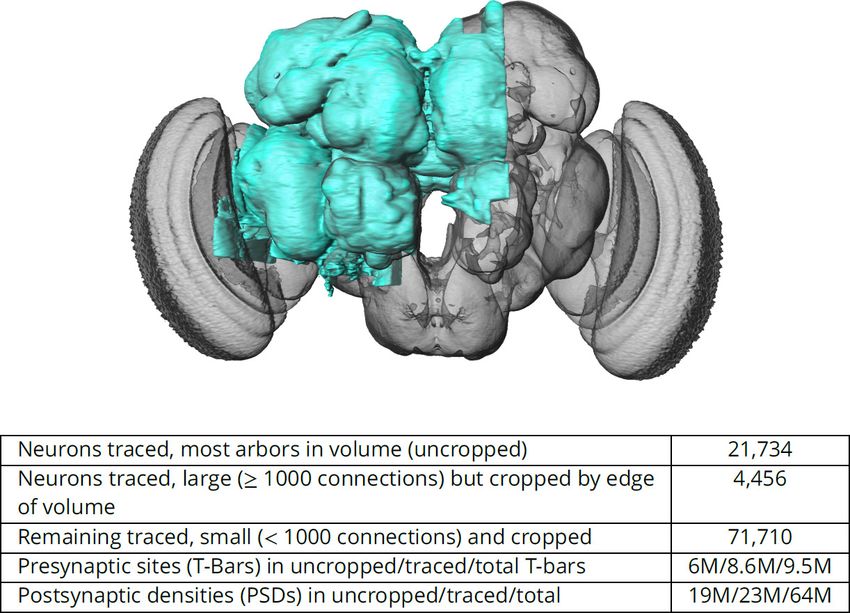
Research article                                                                        Computational and Systems Biology Neuroscience

 PVLP(R)      Posterior ventrolateral protocerebrum     NO3(R)/(L)     Nodulus 3

 PLP(R)       Posterior lateral cerebrum

 WED(R)       Wedge

                                       available, to allow reproducibility of older analyses, but we strongly recommend all new analyses use
                                       the latest version. The analyses in this article, and in the corresponding articles on the mushroom
                                       body and central complex, are based on version v1.1, unless otherwise noted.

                                       What is not included
                                       This research focused on the neurons of the brain and the chemical synapses between them. Every
                                       step in our process, from staining and sample preparation through segmentation and proofreading,
                                       has been optimized with this goal in mind. While neurons and their chemical synapses are critical to
                                       brain operation, they are far from the full story. Other contributors, known to be important, could
                                       not be included in our study, largely for technical reasons. Among these are gap junctions, glia, and
                                       structures internal to the cell such as mitochondria. Gap junctions, or electrical connections between
                                       neurons, are difficult to reliably detect by FIB-SEM under the best of circumstances and not detect-
                                       able at the low (for EM) resolution needed to complete this study in a reasonable amount of time.

                                       Table 2. Regions with 50% included in the hemibrain, sorted by completion percentage.
                                       The approximate percentage of the region included in the hemibrain volume is shown as ‘%inV’. ‘T-
                                       bars’ gives a rough estimate of the size of the region. ‘comp%’ is the fraction of the post-synaptic
                                       densities (PSDs) contained in the brain region for which both the PSD and the corresponding T-bar
                                       are in neurons marked ‘Traced’.
                                       Name           %inV           T-bars        comp%          Name          %inV        T-bars        comp%
                                       PED(R)         100%           54805         85%            aL(R)         100%        95375         84%
                                       b’L(R)         100%           67695         83%            bL(R)         100%        71112         83%
                                       gL(R)          100%           176785        83%            a’L(R)        100%        39091         82%
                                       EB             100%           164286        81%            bL(L)         56%         58799         81%
                                       NO             100%           36722         79%            b’L(L)        88%         57802         78%
                                       gL(L)          55%            133256        76%            CA(R)         100%        69517         73%
                                       AB(R)          100%           2734          65%            aL(L)         51%         44803         62%
                                       FB             100%           451031        62%            AL(R)         83%         501004        59%
                                       AB(L)          100%           572           57%            PB            100%        46557         55%
                                       AME(R)         100%           6045          51%            BU(R)         100%        9385          46%
                                       CRE(R)         100%           137946        40%            AOTU(R)       100%        92578         38%
                                       LAL(R)         100%           234388        38%            SMP(R)        100%        510937        34%
                                       PVLP(R)        100%           475219        30%            ATL(R)        100%        25472         29%
                                       SPS(R)         100%           253818        29%            ATL(L)        100%        28153         29%
                                       VES(R)         84%            157168        29%            IB            100%        200447        28%
                                       CRE(L)         90%            132656        28%            SIP(R)        100%        187493        26%
                                       BU(L)          52%            7014          26%            GOR(R)        100%        27140         26%
                                       WED(R)         100%           232898        25%            SMP(L)        100%        460784        26%
                                       EPA(R)         100%           31438         26%            PLP(R)        100%        429949        26%
                                       AVLP(R)        100%           630538        23%            ICL(R)        100%        202549        23%
                                       SLP(R)         100%           487795        23%            LO(R)         64%         855251        22%
                                       SCL(R)         100%           189569        22%            GOR(L)        60%         19558         21%
                                       LH(R)          100%           231662        19%            CAN(R)        68%         6512          16%

Scheffer, Xu, Januszewski, et al. eLife 2020;9:e57443. DOI: https://doi.org/10.7554/eLife.57443                                           6 of 83
Research article                                                                       Computational and Systems Biology Neuroscience

                                    Their contribution to the connectome will need to be established through other means - see the sec-
                                    tion on future research. Glial cells were difficult to segment, due to both staining differences and
                                    convoluted morphologies. We identified the volumes where they exist (a glia ’mask’, which allows
                                    these regions to be color-coded when viewed in NeuroGlancer) but did not separate them into cells.
                                    Structures internal to the neurons, except for synapses, are not considered here even though many
                                    are visible in our EM preparation. The most obvious example is mitochondria. Again, we have identi-
                                    fied many of them so we could evaluate their effect on segmentation, but they are not included in
                                    our connectome. Finally, autapses (synapses from a neuron onto itself) are known to exist in Dro-
                                    sophila, but are sufficiently rare that they fall well below the rate of false positives in our automated
                                    synapse detection. Therefore most of the putative autapses are false positives, and we do not
                                    include them in our connectivity data.

                                    Differences from connectomes of vertebrates
                                    Most accounts of neurobiology define the operation of the mammalian nervous system with, at
                                    most, only passing reference to invertebrate brains. Fly (or other insect) nervous systems differ from
                                    those of vertebrates in several aspects (Meinertzhagen, 2016b). Some main differences include:
                                       .   Most synapses are polyadic. Each synapse structure comprises a single presynaptic release site
                                           and, adjacent to this, several neurites expressing neurotransmitter receptors. An element,
                                           T-shaped and typically called a T-bar in flies, marks the site of transmitter release into the cleft
                                           between cells. This site typically abuts the neurites of several other cells, where a postsynaptic
                                           density (PSD) marks the receptor location.
                                       .   Most neurites are neither purely axonic nor dendritic, but have both pre- and postsynaptic
                                           partners, a feature that may be more prominent in mammalian brains than recognized
                                           (Morgan and Lichtman, 2020). Within a single brain region, however, neurites are frequently
                                           predominantly dendritic (postsynaptic) or axonic (presynaptic).
                                       .   Unlike some synapses in mammals, EM imagery (at least as we have acquired and analyzed it
                                           here) fails to reveal obvious information about whether a synapse is excitatory or inhibitory.
                                       .   The soma or cell body of each fly neuron resides in a rind (the cell body layer) on the periphery
                                           of the brain, mostly disjoint from the main neurites innervating the internal neuropil. As a
                                           result, unlike vertebrate neurons, no synapses form directly on the soma. The neuronal process
                                           between the soma and the first branch point is called the cell body fiber (CBF), which is like-
                                           wise not involved in the synaptic transmission of information.
                                       .   Synapse sizes are much more uniform than those of mammals. Stronger connections are
                                           formed by increasing the number of synapses in parallel, not by forming larger synapses, as in
                                           vertebrates. In this paper, we will refer to the ‘strength’ of a connection as the synapse count,
                                           even though we acknowledge that we lack information on the relative activity and strength of
                                           the synapses, and thus a true measure of their coupling strength.
                                       .   The brain is small, about 250 mm per side, and has roughly the same size as the dendritic arbor
                                           of a single pyramidal neuron in the mammalian cortex.
                                       .   Axons of fly neurons are not myelinated.
                                       .   Some fly neurons rely on graded transmission (as opposed to spiking), without obvious ana-
                                           tomical distinction. Some neurons even switch between graded and spiking operation
                                           (Pimentel et al., 2016).

                                    Connectome reconstruction
                                    Producing a connectome comprising reconstructed neurons and the chemical synapses between
                                    them required several steps. The first step, preparing a fly brain and imaging half of its center, pro-
                                    duced a dataset consisting of 26 teravoxels of data, each with 8 bits of grayscale information. We
                                    applied numerous machine-learning algorithms and over 50 person-years of proofreading effort over
                                     » 2 calendar years to extract a variety of more compact and useful representations, such as neuron
                                    skeletons, synapse locations, and connectivity graphs. These are both more useful and much smaller
                                    than the raw grayscale data. For example, the connectivity could be reasonably summarized by a
                                    graph with » 25,000 nodes and » 3 million edges. Even when the connections were assigned to dif-
                                    ferent brain regions, such a graph took only 26 MB, still large but roughly a million fold reduction in
                                    data size.

Scheffer, Xu, Januszewski, et al. eLife 2020;9:e57443. DOI: https://doi.org/10.7554/eLife.57443                                          7 of 83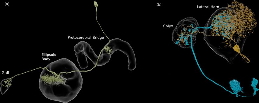
Research article                                                                       Computational and Systems Biology Neuroscience

                                       Many of the supporting methods for this reconstruction have been recently published. Here, we
                                    briefly survey each major area, with more details reported in the companion papers. Major advances
                                    include:
                                       .   New methods to fix and stain the sample, preparing a whole fly brain with well-preserved sub-
                                           cellular detail particularly suitable for machine analysis.
                                       .   Methods that have enabled us to collect the largest EM dataset yet using Focused Ion Beam
                                           Scanning Electron Microscopy (FIB-SEM), resulting in isotropic data with few artifacts, features
                                           that significantly sped up reconstruction.
                                       .   A coarse-to-fine, automated flood-filling network segmentation pipeline applied to image
                                           data normalized with cycle-consistent generative adversarial networks, and an aggressive auto-
                                           mated agglomeration regime enabled by advances in proofreading.
                                       .   A new hybrid synapse prediction method, using two differing underlying techniques, for accu-
                                           rate synapse prediction throughout the volume.
                                       .   New top-down proofreading methods that utilize visualization and machine learning to achieve
                                           orders of magnitude faster reconstruction compared with previous approaches in the fly’s
                                           brain.
                                       Each of these is explained in more detail in the following sections and, where necessary, in the
                                    appendix. The companion papers are ‘The connectome of the Drosophila melanogaster mushroom
                                    body: implications for function’ (Li et al., 2020) and ‘A complete synaptic-resolution connectome of
                                    the Drosophila melanogaster central complex’ by Jayaraman, et al.

                                    Image stack collection
                                    The first steps, fixing and staining the specimen, have been accomplished taking advantage of three
                                    new developments. These improved methods allow us to fix and stain a full fly’s brain but neverthe-
                                    less recover neurons as round profiles with darkly stained synapses, suitable for machine segmenta-
                                    tion and automatic synapse detection. We started with a 5-day-old female of wild-type Canton S
                                    strain G1 x w1118, raised on a 12 hr day/night cycle. 1.5 hr after lights-on, we used a custom-made
                                    jig to microdissect the brain, which was then fixed and embedded in Epon, an epoxy resin. We then
                                    enhanced the electron contrast by staining with heavy metals, and progressively lowered the tem-
                                    perature during dehydration of the sample. Collectively, these methods optimize morphological
                                    preservation, allow full-brain preparation without distortion (unlike fast freezing methods), and pro-
                                    vide increased staining intensity that speeds the rate of FIB-SEM imaging (Lu et al., 2019).
                                        The hemibrain sample is roughly 250  250  250 mm, larger than we can FIB-SEM without intro-
                                    ducing milling artifacts. Therefore, we subdivided our epoxy-embedded samples into 20-mm-thick
                                    slabs, both to avoid artifacts and allow imaging in parallel (each slab can be imaged in a different
                                    FIB machine) for increased throughput. To be effective, the cut surfaces of the slabs must be smooth
                                    at the ultrastructural level and have only minimal material loss. Specifically, for connectomic research,
                                    all long-distance processes must remain traceable across sequential slabs. We used an improved ver-
                                    sion of our previously published ‘hot-knife’ ultrathick sectioning procedure (Hayworth et al., 2015)
                                    which uses a heated, oil-lubricated diamond knife, to section the Drosophila brain into 37 sagittal
                                    slabs of 20 mm thickness with an estimated material loss between consecutive slabs of only ~30 nm –
                                    sufficiently small to allow tracing of long-distance neurites. Each slab was re-embedded, mounted,
                                    and trimmed, then examined in 3D with X-ray tomography to check for sample quality and establish
                                    a scale factor for Z-axis cutting by FIB. The resulting slabs were FIB-SEM imaged separately (often in
                                    parallel, in different FIB-SEM machines), and the resulting volume datasets were stitched together
                                    computationally.
                                        Connectome studies come with clearly defined resolution requirements – the finest neurites must
                                    be traceable by humans and should be reliably segmented by automated algorithms
                                    (Januszewski et al., 2018). In Drosophila, the very finest neural processes are usually 50 nm but can
                                    be as little as 15 nm (Meinertzhagen, 2016a). This fundamental biological dimension determines
                                    the minimum isotropic resolution requirements for tracing neural circuits. To meet the demand for
                                    high isotropic resolution and large volume imaging, we chose the FIB-SEM imaging platform, which
                                    offers high isotropic resolution (
Research article                                                                       Computational and Systems Biology Neuroscience

                                    and isotropic resolution. This allows higher quality automated segmentation and makes manual
                                    proofreading and correction easier and faster.
                                        At the beginning, deficiencies in imaging speed and system reliability of any commercial FIB-SEM
                                    system capped the maximum possible image volume to less than 0.01% of a full fly brain, problems
                                    that persist even now. To remedy them, we redesigned the entire control system, improved the
                                    imaging speed more than 10x, and created innovative solutions addressing all known failure modes,
                                    which thereby expanded the practical imaging volume of conventional FIB-SEM by more than four
                                    orders of magnitude from 103 m3 to 3  107 m3 , while maintaining an isotropic resolution of 8  8
                                    8 nm voxels (Xu et al., 2017; Xu et al., 2020a). In order to overcome the aberration of a large field
                                    of view (up to 300 mm wide), we developed a novel tiling approach without sample stage movement,
                                    in which the imaging parameters of each tile are individually optimized through an in-line auto focus
                                    routine without overhead (Xu et al., 2020b). After numerous improvements, we have transformed
                                    the conventional FIB-SEM from a laboratory tool that is unreliable for more than a few days of imag-
                                    ing to a robust volume EM platform with effective long-term reliability, able to perform years of con-
                                    tinuous imaging without defects in the final image stack. Imaging time, rather than FIB-SEM
                                    reliability, is now the main impediment to obtaining even larger volumes.
                                        In our study here, the Drosophila ’hemibrain’, 13 consecutive hot-knifed slabs were imaged using
                                    two customized enhanced FIB-SEM systems, in which an FEI Magnum FIB column was mounted at
                                    90˚ upon a Zeiss Merlin SEM. After data collection, streaking artifacts generated by secondary elec-
                                    trons along the FIB milling direction were computationally removed using a mask in the frequency
                                    domain. The image stacks were then aligned using a customized version of the software platform
                                    developed for serial section transmission electron microscopy (Zheng et al., 2018; Khairy et al.,
                                    2018), followed by binning along the z-axis to form the final 8  8  8 nm3 voxel datasets. Milling
                                    thickness variations in the aligned series were compensated using a modified version of the method
                                    described by Hanslovsky et al., 2017, with the absolute scale calibrated by reference to the
                                    MicroCT images.
                                        The 20 mm slabs generated by the hot-knife sectioning were re-embedded in larger plastic tabs
                                    prior to FIB-SEM imaging. To correct for the warping of the slab that can occur in this process, meth-
                                    ods adapted from Kainmueller (Kainmueller et al., 2008) were used to find the tissue-plastic inter-
                                    face and flatten each slab’s image stack.
                                        The series of flattened slabs was then stitched using a custom method for large-scale deformable
                                    registration to account for deformations introduced during sectioning, imaging, embedding, and
                                    alignment (Saalfeld et al. in prep). These volumes were then contrast adjusted using slice-wise con-
                                    trast limited adaptive histogram equalization (CLAHE) (Pizer et al., 1987), and converted into a ver-
                                    sioned database (Distributed, Versioned, Image-oriented Database, or DVID) (Katz and Plaza,
                                    2019), which formed the raw data for the reconstruction, as illustrated in Figure 2.

                                    Automated segmentation
                                    Computational reconstruction of the image data was performed using flood-filling networks (FFNs)
                                    trained on roughly five billion voxels of volumetric ground truth contained in two tabs of the hemi-
                                    brain dataset (Januszewski et al., 2018). Initially, the FFNs generalized poorly to other tabs of the
                                    hemibrain, whose image content had different appearances. Therefore, we adjusted the image con-
                                    tent to be more uniform using cycle-consistent generative adversarial networks (CycleGANs)
                                    (Zhu et al., 2017). Specifically, ‘generator’ networks were trained to alter image content such that a
                                    second ‘discriminator’ network was unable to distinguish between image patches sampled from, for
                                    example, a tab that contained volumetric training data versus a tab that did not. A cycle-consistency
                                    constraint was used to ensure that the image transformations preserved ultrastructural detail. The
                                    improvement is illustrated in Figure 3. Overall, this allowed us to use the training data from just two
                                    slabs, as opposed to needing training data for each slab.
                                        FFNs were applied to the CycleGAN-normalized data in a coarse-to-fine manner at 32  32  32
                                    nm3 and 16  16  16 nm3, and to the CLAHE-normalized data at the native 8  8  8 nm3 resolu-
                                    tion, in order to generate a base segmentation that was largely over-segmented. We then agglomer-
                                    ated the base segmentation, also using FFNs. We aggressively agglomerated segments despite
                                    introducing a substantial number of erroneous mergers. This differs from previous algorithms, which
                                    studiously avoided merge errors since they were so difficult to fix. Here, advances in proofreading

Scheffer, Xu, Januszewski, et al. eLife 2020;9:e57443. DOI: https://doi.org/10.7554/eLife.57443                                          9 of 83
Research article                                                                         Computational and Systems Biology Neuroscience

Figure 2. The 13 slabs of the hemibrain, each flattened and co-aligned. A vertical section at the level of the fan-shaped body is shown. Colors are
arbitrary and added to the monochrome data to show brain regions, as defined below. Scale bar 50 mm.

Scheffer, Xu, Januszewski, et al. eLife 2020;9:e57443. DOI: https://doi.org/10.7554/eLife.57443                                                 10 of 83
Research article                                                                       Computational and Systems Biology Neuroscience

Figure 3. Examples of results of CycleGAN processing. (a) Original EM data from tab 34 at a resolution of 16 nm / resolution, (b) EM data after
CycleGAN processing, (c–d) FFN segmentation results with the 16 nm model applied to original and processed data, respectively. Scale bar in (a)
represents 1 mm.

                                    methodology described later in this report enabled efficient detection and correction of such
                                    mergers.
                                       We evaluated the accuracy of the FFN segmentation of the hemibrain using metrics for expected
                                    run length (ERL) and false merge rate (Januszewski et al., 2018). The base segmentation (i.e. the
                                    automated reconstruction prior to agglomeration) achieved an ERL of 163 mm with a false merge

Scheffer, Xu, Januszewski, et al. eLife 2020;9:e57443. DOI: https://doi.org/10.7554/eLife.57443                                              11 of 83
Research article Computational and Systems Biology Neuroscience
rate of 0.25%. After (automated) agglomeration, run length increased to 585 mm but with a false
merge rate of 27.6% (i.e. nearly 30% of the path length was contained in segments with at least one
merge error). We also evaluated a subset of neurons in the volume, ~500 olfactory PNs and mush-
room body KCs chosen to roughly match the evaluation performed in Li et al., 2019 which yielded
an ERL of 825 mm at a 15.9% false merge rate.
Synapse prediction
Accurate synapse identification is central to our analysis, given that synapses form both a critical
component of a connectome and are required for prioritizing and guiding the proofreading effort.
Synapses in Drosophila are typically polyadic, with a single presynaptic site (a T-bar) contacted by
multiple receiving dendrites (most with PSDs) as shown in Figure 4A. Initial synapse prediction
revealed that there are over 9 million T-bars and 60 million PSDs in the hemibrain. Manually validat-
ing each one, assuming a rate of 1000 connections annotated per trained person, per day, would
have taken more than 230 working years. Given this infeasibility, we developed machine learning
approaches to predict synapses as detailed below. The results of our prediction are shown in
Figure 4B, where the predicted synapse sites clearly delineate many of the fly brain regions.
Given the size of the hemibrain image volume, a major challenge from a machine learning per-
spective is the range of varying image statistics across the volume. In particular, model performance
can quickly degrade in regions of the data set with statistics that are not well-captured by the train-
ing set (Buhmann et al., 2019).
To address this challenge, we took an iterative approach to synapse prediction, interleaving
model re-training with manual proofreading, all based on previously reported methods
(Huang et al., 2018). Initial prediction, followed by proofreading, revealed a number of false posi-
tive predictions from structures such as dense core vesicles which were not well-represented in the
original training set. A second filtering network was trained on regions causing such false positives,
Figure 4. Well-preserved membranes, darkly stained synapses, and smooth round neurite profiles are characteristics of the hemibrain sample. Panel (A)
shows polyadic synapses, with a red arrow indicating the presynaptic T-bar, and white triangles pointing to the PSDs. We identified in total 64 million
PSDs and 9.5 million T-bars in the hemibrain volume (Figure 1). Thus the average number of PSDs per T-bar in our sample is 6.7. Mitochondria (‘M’),
synaptic vesicles (‘SV’), and the scale bar (0.5 mm) are shown. Panel (B) shows a horizontal cross section through a point cloud of all detected synapses.
This EM point cloud defines many of the compartments in the fly’s brain, much like an optical image obtained using antibody nc82 (an antibody against
Bruchpilot, a component protein of T-bars) to stain synapses. This point cloud is used to generate the transformation from our sample to the standard
Drosophila brain.
Scheffer, Xu, Januszewski, et al. eLife 2020;9:e57443. DOI: https://doi.org/10.7554/eLife.57443 12 of 83Research article Computational and Systems Biology Neuroscience
and used to prune back the original set of predictions. We denote this pruned output as the ‘initial’
set of synapse predictions.
Based on this initial set, we began collecting human-annotated dense ground-truth cubes
throughout the various brain regions of the hemibrain, to assess variation in classifier performance
by brain region. From these cubes, we determined that although many regions had acceptable pre-
cision, there were some regions in which recall was lower than desired. Consequently, a subset of
cubes available at that time was used to train a new classifier focused on addressing recall in the
problematic regions. This new classifier was used in an incremental (cascaded) fashion, primarily by
adding additional predictions to the existing initial set. This gave better performance than complete
replacement using only the new classifier, with the resulting predictions able to improve recall while
largely maintaining precision.
As an independent check on synapse quality, we also trained a separate classifier
(Buhmann et al., 2019), using a modified version of the ‘synful’ software package. Both synapse pre-
dictors give a confidence value associated with each synapse, a measure of how firmly the classifier
believes the prediction to be a true synapse. We found that we were able to improve recall by taking
the union of the two predictor’s most confident synapses, and similarly improve precision by remov-
ing synapses that were low confidence in both predictions. Figure 5A and B show the results, illus-
trating the precision and recall obtained in each brain region.
Figure 5. Precision and recall for synapse prediction, panel (A) for T-bars, and panel (B) for synapses as a whole including the identification of PSDs. T-
bar identification is better than PSD identification since this organelle is both more distinct and typically occurs in larger neurites. Each dot is one brain
region. The size of the dot is proportional to the volume of the region. Humans proofreaders typically achieve 0.9 precision/recall on T-bars and 0.8
precision/recall on PSDs, indicated in purple. Data available in Figure 5—source datas 1–2.
The online version of this article includes the following source data for figure 5:
Source data 1. Data for Figure 5A.
Source data 2. Data for Figure 5B.
Scheffer, Xu, Januszewski, et al. eLife 2020;9:e57443. DOI: https://doi.org/10.7554/eLife.57443 13 of 83Research article Computational and Systems Biology Neuroscience
Proofreading
Since machine segmentation is not perfect, we made a concerted effort to fix the errors remaining
at this stage by several passes of human proofreading. Segmentation errors can be roughly grouped
into two classes - ‘false merges’, in which two separate neurons are mistakenly merged together,
and ‘false splits’, in which a single neuron is mistakenly broken into several segments. Enabled by
advances in visualization and semi-automated proofreading using our Neu3 tool (Hubbard et al.,
2020), we first addressed large false mergers. A human examined each putative neuron and deter-
mined if it had an unusual morphology suggesting that a merge might have occurred, a task still
much easier for humans than machines. If judged to be a false merger, the operator identified dis-
crete points that should be on separate neurons. The shape was then resegmented in real time
allowing users to explore other potential corrections. Neurons with more complex problems were
then scheduled to be re-checked, and the process repeated until few false mergers remained.
In the next phase, the largest remaining pieces were merged into neuron shapes using a combi-
nation of machine-suggested edits (Plaza, 2014) and manual intuition, until the main shape of each
neuron emerged. This requires relatively few proofreading decisions and has the advantage of pro-
ducing an almost complete neuron catalog early in the process. As discussed below, in the section
on validation, emerging shapes were compared against genetic/optical image libraries (where avail-
able) and against other neurons of the same putative type, to guard against large missing or super-
fluous branches. These procedures (which focused on higher-level proofreading) produced a
reasonably accurate library of the main branches of each neuron, and a connectome of the stronger
neuronal pathways. At this point, there was still considerable variations among the brain regions,
with greater completeness achieved in regions where the initial segmentation performed better.
Finally, to achieve the highest reconstruction completeness possible in the time allotted, and to
enable confidence in weaker neuronal pathways, proofreaders connected remaining isolated frag-
ments (segments) to already constructed neurons, using NeuTu (Zhao et al., 2018) and Neu3
(Hubbard et al., 2020). The fragments that would result in largest connectivity changes were consid-
ered first, exploiting automatic guesses through focused proofreading where possible. Since proof-
reading every small segment is still prohibitive, we tried to ensure a basic level of completeness
throughout the brain with special focus in regions of particular biological interest such as the central
complex and mushroom body.
Figure 6. Division of the sample into brain regions. (A) A vertical section of the hemibrain dataset with synapse point clouds (white), predicted glial
tissue (green), and predicted fiber bundles (magenta). (B) Grayscale image overlaid with segmented neuropils at the same level as (A). (C) A frontal view
of the reconstructed neuropils. Scale bar: (A, B) 50 mm.
Scheffer, Xu, Januszewski, et al. eLife 2020;9:e57443. DOI: https://doi.org/10.7554/eLife.57443 14 of 83Research article Computational and Systems Biology Neuroscience
Defining brain regions
In a parallel effort to proofreading, the sample was annotated with discrete brain regions. Our pro-
gression in mapping the cells and circuits of the fly’s brain bears formal parallels to the history of
mapping the earth, with many territories that are named and with known circuits, and others that still
lack all or most of these. For the hemibrain dataset, the regions are based on the brain atlas in
Ito et al., 2014. The dataset covers most of the right hemisphere of the brain, except the optic lobe
(OL), periesophageal neuropils (PENP) and gnathal ganglia (GNG), as well as part of the left hemi-
sphere (Table 2). It covers about 36% of all synaptic neuropils by volume, and 54% of the central
brain neuropils. We examined innervation patterns, synapse distribution, and connectivity of recon-
structed neurons to define the neuropils as well as their boundaries on the dataset. We also made
necessary, but relatively minor, revisions to some boundaries by considering anatomical features
that had not been known during the creation of previous brain maps, while following the existing
structural definitions (Ito et al., 2014). We also used information from synapse point clouds, a pre-
dicted glial mask, and a predicted fiber bundle mask to determine boundaries of the neuropils
(Figure 6A). The brain regions of the fruit fly (Figure 6, B and C) include synaptic neuropils and non-
synaptic fiber bundles. The non-synaptic cell body layer on the brain surface, which contains cell
bodies of the neurons and some glia, surrounds these structures. The synaptic neuropils can be fur-
ther categorized into two groups: delineated and diffuse neuropils. The delineated neuropils have
distinct boundaries throughout their surfaces, often accompanied by glial processes, and have clear
internal structures in many cases. They include the antennal lobe (AL), bulb (BU), as well as the neu-
ropils in the optic lobe (OL), mushroom body (MB), and central complex (CX). Remaining are the dif-
fuse neuropils, sometimes referred to as terra incognita, since most have been less investigated than
the delineated neuropils.
Diffuse (terra incognita) neuropils
In the previous brain atlas of 2014, boundaries of some terra incognita neuropils were somewhat
arbitrarily determined, due to a lack of precise information of the landmark neuronal structures used
for the boundary definition. In the hemibrain data, we adjusted these boundaries to trace more faith-
fully the contours of the structures that are much better clarified by the EM-reconstructed data.
Examples include the lateral horn (LH), ventrolateral neuropils (VLNP), and the boundary between
the crepine (CRE) and lateral accessory lobe (LAL). The LH has been defined as the primary projec-
tion target of the olfactory projection neurons (PNs) from the antennal lobe (AL) via several antennal
lobe tracts (ALTs) (Ito et al., 2014; Pereanu et al., 2010). The boundary between the LH and its sur-
rounding neuropils is barely visible with synaptic immunolabeling such as nc82 or predicted synapse
point clouds, as the synaptic contrast in these regions is minimal. The olfactory PNs can be grouped
into several classes, and the projection sites of the uniglomerular PNs that project through the
medial ALT (mALT), the thickest fiber bundle between the AL and LH, give the most conservative
and concrete boundary of the ‘core’ LH (Figure 7A). Multiglomerular PNs, on the other hand, proj-
ect to much broader regions, including the volumes around the core LH (Figure 7B). These regions
include areas which are currently considered parts of the superior lateral protocerebrum (SLP) and
posterior lateral protocerebrum (PLP). Since the ‘core’ LH roughly approximates the shape of the tra-
ditional LH, and the boundaries given by the multiglomerular PNs are rather diffused, in this study
we assumed the core to be the LH itself. Of course, the multiglomerular PNs convey olfactory infor-
mation as well, and therefore the neighboring parts of the SLP and PLP to some extent also receive
inputs from the antennal lobe. These regions might be functionally distinct from the remaining parts
of the SLP or PLP, but they are not explicitly separated from those neuropils in this study.
The VLNP is located in the lateral part of the central brain and receives extensive inputs from the
optic lobe through various types of the visual projection neurons (VPNs). Among them, the projec-
tion sites of the lobula columnar (LC), lobula plate columnar (LPC), lobula-lobula plate columnar
(LLPC), and lobula plate-lobula columnar (LPLC) cells form characteristic glomerular structures, called
optic glomeruli (OG), in the AOTU, PVLP, and PLP (Klapoetke et al., 2017; Otsuna and Ito, 2006;
Panser et al., 2016; Wu et al., 2016). We exhaustively identified columnar VPNs and found 41 types
of LC, two types of LPC, six types of LLPC, and three types of LPLC cells (including sub-types of pre-
viously identified types). The glomeruli of these pathways were used to determine the medial bound-
ary of the PVLP and PLP, following existing definitions (Ito et al., 2014), except for a few LC types
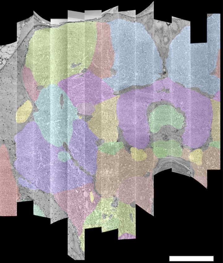
Scheffer, Xu, Januszewski, et al. eLife 2020;9:e57443. DOI: https://doi.org/10.7554/eLife.57443 15 of 83Research article Computational and Systems Biology Neuroscience Figure 7. Reconstructed brain regions and substructures. (A, B) Dorsal views of the olfactory projection neurons (PNs) and the innervated neuropils, AL, CA, and LH. Uniglomerular PNs projecting through the mALT are shown in (A), and multiglomerular PNs are shown in (B). (C, D) Columnar visual projection neurons. Each subtype of cells is color coded. LC cells are shown in (C), and LPC, LLPC, and LPLC cells are shown in (D). (E, F) The nine layers of the fan-shaped body (FB), along with the asymmetrical bodies (AB) and the noduli (NO), displayed as an anterior-ventral view (E), and a lateral Figure 7 continued on next page Scheffer, Xu, Januszewski, et al. eLife 2020;9:e57443. DOI: https://doi.org/10.7554/eLife.57443 16 of 83
Research article                                                                           Computational and Systems Biology Neuroscience

Figure 7 continued
view (F). In (E), three FB tangential cells (FB1D (blue), FB3A (green), FB8H (purple)) are shown as markers of the corresponding layers (FBl1, FBl3, and
FBl8, respectively). (G) Zones in the ellipsoid body (EB) defined by the innervation patterns of different types of ring neurons. In this horizontal section
of the EB, the left side shows the original grayscale data, and the seven ring neuron zones (see Table 1) are color-coded. The right side displays the
seven segmented zones based on the innervation pattern, in a slightly different section. Scale bar: 20 mm.

                                      which do not form glomerular terminals. The terminals of the reconstructed LC cells and other lobula
                                      complex columnar cells (LPC, LLPC, LPLC) are shown in Figure 7C and D, respectively.
                                         In the previous paper (Ito et al., 2014), the boundary between the CRE and LAL was defined as
                                      the line roughly corresponding to the posterior-ventral surface of the MB lobes, since no other
                                      prominent anatomical landmarks were found around this region. In this dataset, we found several
                                      glomerular structures surrounding the boundary both in the CRE and LAL. These structures include
                                      the gall (GA), rubus (RUB), and round body (ROB). Most of them turned out to be projection targets
                                      of several classes of central complex neurons, implying the ventral CRE and dorsal LAL are closely
                                      related in their function. We re-determined the boundary so that each of the glomerular structures
                                      would not be divided into two, while keeping the overall architecture and definition of the CRE and
                                      LAL. The updated boundary passes between the dorsal surface of the GA and the ventral edge of
                                      the ROB. Other glomerular structures, including the RUB, are included in the CRE.

                                      Delineated neuropils
                                      Substructures of the delineated neuropils have also been added to the brain region map in the hemi-
                                      brain. The asymmetrical bodies (AB) were added as the fifth independent neuropil of the CX
                                      (Wolff and Rubin, 2018). The AB is a small synaptic volume adjacent to the ventral surface of the
                                      fan-shaped body (FB) that has historically been included in the FB (Ito et al., 2014). The AB has
                                      been described as a Fasciclin II (FasII)-positive structure that exhibits left-right structural asymmetry
                                      by Pascual et al., 2004, who reported that most flies have their AB only in the right hemisphere,
                                      while a small proportion (7.6%) of wild-type flies have their AB on both sides. In the hemibrain data-
                                      set, the pair of ABs is situated on both sides of the midline, but the left AB is notably smaller than
                                      the right AB (right: 1679 mm3, left: 526 mm3), still showing an obvious left-right asymmetry. The
                                      asymmetry is consistent with light microscopy data (Wolff and Rubin, 2018), though the absolute
                                      sizes differ, with the light data showing averages (n = 21) of 522 mm3 for the right and 126 mm3 on
                                      the left. The AB is especially strongly connected to the neighboring neuropil, the FB, by neurons
                                      including vDeltaA_a (anatomical name AF in Wolff and Rubin, 2018), while it also houses both pre-
                                      and postsynaptic terminals of the CX output neurons such as the subset of FS4A and FS4B neurons
                                      that project to AB. These anatomical observations imply that the AB is a ventralmost annexed part
                                      of the FB, although this possibility is neither developmentally nor phylogenetically proven.
                                         The round body (ROB) is also a small round synaptic structure situated on the ventral limit of the
                                      crepine (CRE), close to the b lobe of the MB (Lin et al., 2013; Wolff and Rubin, 2018). It is a glo-
                                      merulus-like structure and one of the foci of the CX output neurons, including the PFR (protocerebral
                                      bridge – fan-shaped body – round body) neurons. It is classified as a substructure of the CRE along
                                      with other less-defined glomerular regions in the neuropil, many of which also receive signals from
                                      the CX. Among these, the most prominent one is the rubus (RUB). The ROB and RUB are two dis-
                                      tinct structures; the RUB is embedded completely within the CRE, while the ROB is located on the
                                      ventrolateral surface of the CRE. The lateral accessory lobe (LAL), neighboring the CRE, also houses
                                      similar glomerular terminals, and the gall (GA) is one of them. While the ROB and GA have relatively
                                      clear boundaries separating them from the surrounding regions, they may not qualify as indepen-
                                      dent neuropils because of their small size and the structural similarities with the glomerulus-like ter-
                                      minals around them. They may be comparable with other glomerular structures such as the AL
                                      glomeruli and the optic glomeruli in the lateral protocerebrum, both of which are considered as sub-
                                      structures of the surrounding neuropils.
                                         Substructures of independent neuropils are also defined using neuronal innervations. The five MB
                                      lobes on the right hemisphere are further divided into 15 compartments (a1–3, a’1–3, b1–2, b’1–2,
                                      and g1–5) (Tanaka et al., 2008; Aso et al., 2014) by the mushroom body output neurons (MBONs)
                                      and dopaminergic neurons (DANs). Our compartment boundaries were defined by approximating
                                      the innervation of these neurons. Although the innervating regions of the MBONs and DANs do not

Scheffer, Xu, Januszewski, et al. eLife 2020;9:e57443. DOI: https://doi.org/10.7554/eLife.57443                                                      17 of 83
You can also read