11432 Causality in the link between income and satisfaction. IV estimation with internal instruments
←
→
Page content transcription
If your browser does not render page correctly, please read the page content below
1143

                                       2021

Causality in the link between income
and satisfaction. IV estimation with
internal instruments

Susanne Elsas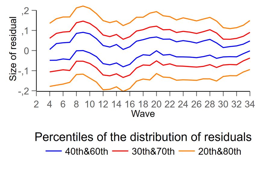
SOEPpapers on Multidisciplinary Panel Data Research at DIW Berlin

This series presents research findings based either directly on data from the German Socio-
Economic Panel (SOEP) or using SOEP data as part of an internationally comparable data
set (e.g. CNEF, ECHP, LIS, LWS, CHER/PACO). SOEP is a truly multidisciplinary household
panel study covering a wide range of social and behavioral sciences: economics, sociology,
psychology, survey methodology, econometrics and applied statistics, educational science,
political science, public health, behavioral genetics, demography, geography, and sport
science.

The decision to publish a submission in SOEPpapers is made by a board of editors chosen
by the DIW Berlin to represent the wide range of disciplines covered by SOEP. There is no
external referee process and papers are either accepted or rejected without revision. Papers
appear in this series as works in progress and may also appear elsewhere. They often
represent preliminary studies and are circulated to encourage discussion. Citation of such a
paper should account for its provisional character. A revised version may be requested from
the author directly.

Any opinions expressed in this series are those of the author(s) and not those of DIW Berlin.
Research disseminated by DIW Berlin may include views on public policy issues, but the
institute itself takes no institutional policy positions.

The SOEPpapers are available at http://www.diw.de/soeppapers

Editors:
Jan Goebel (Spatial Economics)
Stefan Liebig (Sociology)
David Richter (Psychology)
Carsten Schröder (Public Economics)
Jürgen Schupp (Sociology)
Sabine Zinn (Statistics)

Conchita D’Ambrosio (Public Economics, DIW Research Fellow)
Denis Gerstorf (Psychology, DIW Research Fellow)
Katharina Wrohlich (Gender Economics)
Martin Kroh (Political Science, Survey Methodology)
Jörg-Peter Schräpler (Survey Methodology, DIW Research Fellow)
Thomas Siedler (Empirical Economics, DIW Research Fellow)
C. Katharina Spieß (Education and Family Economics)
Gert G. Wagner (Social Sciences)

ISSN: 1864-6689 (online)
German Socio-Economic Panel (SOEP)
DIW Berlin
Mohrenstrasse 58
10117 Berlin, Germany

Contact: soeppapers@diw.de
Causality in the link between income and satisfaction.
                      IV estimation with internal instruments

                 Causality in the link between income and satisfaction.
                      IV estimation with internal instruments 1

                                                 Susanne Elsas
              ifb · State Institute for Family Research at the University of Bamberg, Germany

Abstract
Usually, it is expected that income increases life satisfaction. In recent years tough, research
emerged that shows how subjective well-being, including satisfaction, influences objective mea-
sures, as for example income. This would then require explicit identification strategies for esti-
mating effects of income on life satisfaction.
    I address this issue using German SOEP data and Lewbel’s (2012) method, which generates
instruments from heteroscedasticity. This allows identification of two separate causal effects
in the link between income and life satisfaction: (1) income affecting satisfaction and (2) sat-
isfaction affecting income. This analysis focuses on life satisfaction and equivalized income,
because this is the income measure most welfare analyses use to assess utility of income.
    Results show no significant effects of income on life satisfaction, but effects of satisfaction
on income. This suggest that the effect of income on life satisfaction may be overstated in
standard approaches that do not account for this reverse causality – possibly due to reverse
causality, which is likely rooted in response behavior, rather than income generation.

Acknowledgements: I am very grateful to Caspar Kaiser who spontaneously joined (yet in the
end left) this project; furthermore, I thank F. Sarracino, Ch. Wunder, G. Heineck, M. Gebel
and participants of the ISQOLS Conference in Granada and the Empirical Micro Economics
Meeting in Leipzig for helpful comments on earlier drafts.

Keywords: life satisfaction, income, utility of income, reverse causality.

 1   The main idea, general set up and most results of this study are part of my thesis (Elsas 2021), but not Sec-
     tion 5.3 and the conclusion related to it.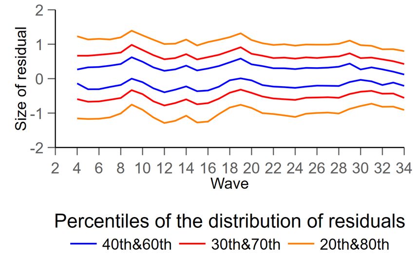
1    Introduction
In economic theory, the concept of utility is used to explain human behavior. It is standardly
assumed that higher incomes generate higher levels of utility. Since utility is a theoretical con-
cept, which is not directly observable, welfare and happiness economists equate utility with
happiness and analyze self-reported data on satisfaction to test this assumption empirically (i.e.
Easterlin 1995, Vendrik and Woltjer 2007, Layard et al. 2008, Carver and Grimes 2019). Typi-
cally the only causal pathway considered is that running from income to happiness. The reverse
pathway, i.e. happiness causing income, is often neglected.
    More recently however, evidence emerged that happiness promotes health, sociability, ca-
reers and productivity (De Neve et al. 2013) - all of which are causes and sources of earned
income. Earned incomes, in turn, are one of the primary elements of a household’s overall in-
come (alongside e.g. government transfers or incomes from capital). These positive effects of
happiness could transmit to overall household income, which means that overall household in-
come could therefore potentially be influenced by happiness. Additionally, happiness may also
increase equivalized household incomes via increasing the probability of household formation
with a partner, which generates economies of scale compared to single households. It is thus
likely that household income is also positively affected by happiness.
    Since most people refer to equivalized household income when evaluating their income
satisfaction (Schwarze 2003), it is reasonable that many studies use measures of equivalized
household income when estimating the hedonic effects of income (e.g., Stutzer 2004, Boyce
et al. 2010, Vendrik and Woltjer 2007, Jäntti et al. 2014). But, if greater happiness is a cause
for greater household incomes, then estimates that do not account for this causal path will be
biased upward. One aim of this study is therefore to explore the probable size of such a bias.
I thus provide here the first (to my knowledge) simultaneous estimations of the bi-directional
causal effects between equivalized income and happiness.
    Estimating the causal effect of happiness on equivalized household income is another sub-
stantive contribution which adds to the wider debate on the effects of happiness on socio-
economic outcomes.

                                                1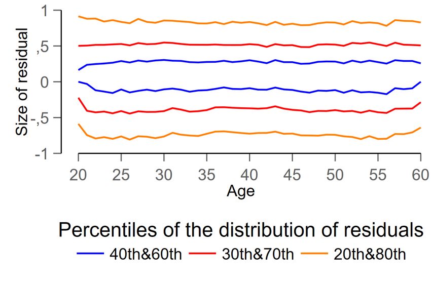
Data for the analysis come from the German SOEP2 for the years 1985 to 2017 (273768
person-year-observations of 38,134 individuals). Self-reports on life satisfaction serve as mea-
sure for happiness, but estimations using financial satisfaction are provided too, since financial
satisfaction is also a commonly used proxy for utility of income. Income is measured as annual
equivalized household income. Identification relies on Lewbel instruments (Lewbel 2012), a
method that exploits heteroscedasticity in the endogenous regressors to identify causal effects.
     Results indicate that income has no significant causal effect on life satisfaction, whereas
satisfaction has an effect on income. Standard estimates of the effect of income on satisfaction
appear to be biased upwards.
     In the next section some related literature is discussed. The economic model, the identifica-
tion strategy and the econometric model are explained in the third section. The fourth section
describes the data. Since this is crucial for identification, that section also describes the patterns
of heteroscedasticity in the endogenous variables of interest. Results are presented in the fifth
section. Two further sections present robustness checks and further estimations using financial
satisfaction. A final section concludes.

2      Related literature
In economic theory and in the general public it is expected that income, ceteris paribus, gen-
erates utility and thereby raises satisfaction.           Although this hypothesis has received general
empirical support, the much debated Easterlin Paradox (Easterlin 1974, Stevenson and Wolfers
2008, Easterlin 2017, Kaiser and Vendrik 2019), which notes that as countries grow richer over
time, they do not grow happier, raises doubts about the utility of income hypothesis.
     The debate about the importance of own income for life satisfaction never stopped com-
pletely (Hagerty and Veenhoven 2003, Easterlin 2005, Clark et al. 2008, Kahneman and Deaton
2010, Boyce et al. 2010), but the majority agrees that income does matter, though perhaps only
to a limited extent (Easterlin 1995, Oswald 1997, Diener and Oishi 2000, Frey and Stutzer 2002,
Boyce et al. 2017).
 2   The German Socio-Economic Panel Study is an ongoing longitudinal study of German households. The SOEP
     began in 1984 with a sample of adult members from randomly selected households in West Germany. Since
     1984, the SOEP has expanded to include East Germany and also added various subsamples to maintain a
     representative sample of the entire German population and to allow analyses of special groups in society, e.g
     affluent households, the migrant population or income-poor families.

                                                        2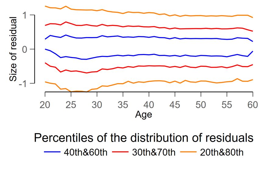
Very few previous studies, though, use methods that are explicitly able to identify causal
effects of income on life satisfaction. Most of these studies find support for the hypothesis that
income matters. At first, in a very innovative approach a significantly positive effect of income
on life satisfaction was estimated exploiting exogenous income increases that occurred with
the German reunification (Frijters et al. 2004). Yet, orderd logit estimations that account for
individual-specific correlated unobserved heterogeneity were lateron found to be inconsistent
estimators (Baetschmann et al. 2015). Some instrumental variable approaches yielded positive
estimates, yet relevance and exogeneity of the instruments for income are not always straightfor-
wardly established. This is, for example, the case if instruments are constructed from the share
of respondents in the household showing their payslip to the interviewer3 and also when the par-
ents’ or spouse’s education is used as an instrument.4 Exogeneity and relevance of industry- and
occupation-wide variation in earnings, in contrast, are very well-established for instrumenting
income in life satisfaction estimations, and are hence repeatedly used for this purpose: Luttmer
(2005) analyzes the effect of spatial reference income, i.e. the mean income in the neigborhood,
using US data. Vendrik (2013) and Kaiser (2018) use the same instruments, but German and
British Data, and analyze if people adapt to income. All three studies did not focus the effect
of own current income on life satisfaction, but all found strongly significant, positive and large
effects of current income on life satisfaction. Vendrik (2013), though, mentions that the instru-
ments they use are specially suitable to predict permanent income, rather than income of shorter
periods.
     In contrast to the aforementioned studies, Lachowska (2017) found large, significantly pos-
itive and robust effects of income on affect, but no statistically significant, nor robust effects on
life satisfaction. She uses an instrument that she constructed from the economic stimulus tax
 3   Powdthavee (2010) used the share of respondents who showed their payslip to the interviewer, to predict house-
     hold income. "The idea is that there is a direct correlation between the proportion of household members
     showing and not showing their payslip to the interviewer and that of household income as household income is
     bound to have been measured more accurately where the proportion of household member who showed payslip
     is high." (Powdthavee 2010, p. 81). This however explains precision of the income measure, but is no argument
     for a monotone effect on the amount of income, which would be needed for an instrumental variable estimation.
 4   Knight et al. (2009) also estimate significantly positive effects of income on life satisfaction in China. They used
     fathers and spouses education to instrument income in the life satisfaction equation. The usual statistical test
     are convincing, but only a weak argument is given that supports the generally untestable exogeneity assumption
     for the instrument: it is said that it was not likely that spouses or fathers education influences life satisfaction
     (except through income), because even own education is only weakly associated to life satisfaction in their
     OLS estimations with all covariates (Knight et al. 2009, p. 646). Findings for Germany indicate the contrary,
     i.e. that "[...] overall, family background and individual factors are of approximately equal importance for
     permanent life satisfaction." (Schnitzlein and Wunder 2016, p. 146)

                                                            3
rebate that was implemented in the US in 2008, where timing of the payment was randomly
assigned. This randomly assigned timing is the exogenous variation that she uses to identify the
causal effect of a one-shot increase in income on life satisfaction.
A further study that analyzes the effects of short-run income shocks and long-term income
changes bridges the gap between those who found large positive effects of income on life sat-
isfaction (Luttmer 2005, Vendrik 2013, Kaiser 2018) and the result of Lachowska (2017), who
found no effect: Using also German SOEP data Bayer and Juessen (2015) found that long-
term changes in income have significant and sizable positive effects on life satisfaction, while
short-term shocks have none. The authors identify the causal effects from lags and leads of the
endogenous regressor.5
Psychologists, economists and common sense suspect that satisfaction or happiness also
impact on income. Several recent studies in behavioral economics analyze (affective and eval-
uative) subjective well-being as a cause of various outcomes such as risk avoidance or delay
gratification (for an overview, see: Lane 2017, De Neve et al. 2013), saving (Guven 2012), ab-
senteeism (Bubonya et al. 2017), (un-)employment (Krause 2013, Kesavayuth and Zikos 2018),
career progression (for an overview see: Walsh et al. 2018) or productivity (Oswald et al. 2015,
Tenney et al. 2016, Bryson et al. 2017, Böckerman and Ilmakunnas 2012). All these outcomes
predict income. Nevertheless, studies of the effect of satisfaction on income are rare and most
often focus on earned income rather than equivalized household income. The first study on
the effect of satisfaction on income appears to be by Graham et al. (2004). Using Russian
panel data, they find that positive expectations and residual happiness are positively associ-
ated to future incomes. However, time lags can only identify unidirectional causal effects if
no individual-specific unobserved heterogeneity is present that affects both dependent and any
explanatory variable. De Neve and Oswald (2012) address this problem with siblings fixed
effects; they estimate the effect of happiness at age 22 on future income at age 29 and find a
positive effect. One other study investigates the causal effect of happiness on earnings (Mishra
and Smyth 2014) using a relatively new method, the Lewbel (2012) instruments. They find a
5 To pass the exogeneity requirement, the instruments must meet two conditions: The “No Foresight” condition
which assumes that all deterministic components of income are captured in the exogenous controls that enter
the first-stage regression. It holds whenever the individual has no better information on income growth in the
next period than the econometrician. The second condition for the instrument to be exogenous is the “Short
Memory” condition, which requires that, narrowly understood, change in assets neither responds to persistent
shocks in the year before, nor to transitory shocks two years before (Bayer and Juessen 2015, pp. 166).
4positive effect of happiness on earnings for men. All these three, however, analyze earned in-
come. This is the main income source for many people. However, these results cannot answer
the question about effects of satisfaction on equivalized income. It could be that the effect of
satisfaction on earnings attenuates when earnings are shared among household members. On
the other hand, it is possible that household formation accelerates the effect of satisfaction on
equivalized household income, which would not be picked up by estimation for earned income.
This would be a minor problem if many studies focusing the utility or welfare effect of
income did not analyze the potential effect of equivalised household income (e.g., Stutzer 2004,
Boyce et al. 2010, Vendrik and Woltjer 2007, Jäntti et al. 2014). For the purpose of welfare
analyses and due to economies of scale, whereby incomes may be used more efficiently in
larger households, it is appropriate in these settings to equivalize household incomes. And it is
hence necessary to know if estimates of the hedonic effect of income are potentially overstated
due to reverse causality that runs from happiness to equivalized household income.
3 Model and identification
To identify causal effects, researchers often exploit time lags, based on the idea that causes pre-
cede results. However, if individual-specific time-invariant unobservable or unobserved char-
acteristics influence income and happiness, the time-lag method could falsely indicate a causal
relation due to confounding. Such problems may be partially cured with fixed effects, like indi-
vidual or family fixed effects. Nevertheless estimates still suffer from time-varying unobserved
heterogeneity, and only the limited variation around fixed effects can be used for identification.
An arguably more elaborate approach applies external instruments, which affect only one
of income or happiness directly, while the second is only indirectly affected via the first. Con-
vincing instruments, especially for satisfaction, are usually hard to find. Guven (2012), who
analyzed the effect of happiness on savings and consumption behavior found a convincing in-
strument for happiness: unexpected sunshine. Sunshine sufficiently influences happiness, so
that the instrument is strong enough to identify sizable effects of happiness on savings behavior.
Yet these might be be restricted to those whose satisfaction answers are driven to a larger extent
by moods, affect and sunshine. As for income, an unforeseen tax rebate as used by Lachowska
(2017) may be a particularly clean instrument, but is not available in the German case.
5Lewbel (2012) shows that it may be an alternative approach to construct internal instruments
from the model’s data. This method can be applied when no valid external instruments are
available and is already used in empirical economics. In the following it will be explained how
Lewbel’s (2012) method can be applied to identify causal effects in the income happiness link.
3.1 Model
It is well-established that utility - measured in levels of stated satisfaction - depends positively
on personal incomes. Nevertheless, there remains a long-standing controversy over the degree
to which satisfaction depends on income. I join this debate with the question:
RQ1: Does satisfaction depend on income?
One might approach answering RQ1 by estimating a regression of the form:
sit = γ1 ln(yit ) + X 0 it β1 + αi + ε1it (1)
Here, sit denotes satisfaction of individual i at time t. X is a vector of controls, αi is an individual
fixed effect, and ε1it is an ideosyncratic error. I avoid estimating α1i , by demeaning6 (1):
˙ ) + Ẋ 0 it β1 + ε1it
ṡit = γ1 ln(y (2)
it
˙ ) and each jth variable ẋ jit of the J variables in Ẋit .
Here, ṡit = sit − s̄i , and similar for ln(yit
Although demeaning captures all time-invariant unobserved determinants that might con-
found the relationship between sit and ln(yit ), there are further issues which could cause inac-
curacies in answers obtained from estimating (2): First, respondents might find it difficult to
accurately report their incomes. There may therefore be measurement error in income, caus-
ing estimates from (2) to be biased towards zero. Second, there may be further unobserved
time-varying determinants of stated satisfaction that could act as confounders. Third, incomes
may depend on satisfaction. Although this third possibility has been considered, most previous
studies purely focused on earned income. Focusing earned income serves more to understand
how satisfaction causes income. This study however attempts to explore if equivalized income
6 I do not manually demean, but use Stata’s xtreg and ivreg2h commands, each with the fe option.
6is also influenced by satisfaction. To the best of my knowledge this possibility has until now
not been evaluated in a joint analysis with RQ1. Therefore, the second research question is:
RQ2: Does equivalized income depend on satisfaction?
A natural approach to answering this question is to estimate a regression that is analogous in
form to (2):
˙ ) = γ2 ṡit + Ẋ 0 it β2 + ε2it
ln(y (3)
it
However, if the true values of γ1 and γ2 are indeed different from zero, OLS estimates of (2)
and (3) will be biased due to simultaneity of γ1 and γ2 . One aim of this study is to gauge how
large the impact of such simultaneity is.
3.2 Identification
A standard approach to circumvent these problems would be to find suitable instruments for
both satisfaction and income. Although such instruments potentially exist (see Section 2), I
here explore the use of an alternative strategy where instruments are constructed from a readily
available subset of the observed exogenous variables in Ẋ. This approach, developed by Lewbel
(2012), can be summarized as follows.
˙ ) in equation (2), the following auxiliary regression are
To construct instruments for ln(yit
run in the first step:7
˙ 0
ln(y)it = Ż it δ1 + ν1it (4)
Where Ż is a subset of K variables in Ẋ with each variable in Ż satisfying the exogeneity
assumption. One can then use the residuals ν̂1it and sample-centered values of each variable żk
in Ż to calculate K instruments for ln(yit ) in the second step:
yinstkit = (żkit − ż¯k )ν̂1it (5)
7 Actually I did not conduct the estimation step by step, I use the Stata-ado ’ivreg2h’ by Baum and Schaffer
(2012).
7Instruments for ṡit to be used in equation (3) are constructed analogously:
ṡit = Ż 0 it δ2 + ν2it (6)
is estimated to calculate the K instruments for ṡit as given by
sinstkit = (żkit − ż¯k )ν̂2it . (7)
These instruments are then - as in conventional instrumental variable estimations - used to
predict the endogenous regressors in the structural equations, (2) and (3).
The intuition of this identification strategy follows from linear regression mechanics: Resid-
uals are by construction exogenous to the the right-hand-side variables. If satisfaction, the out-
come of Eq. (2), is independent of the residuals of the auxiliary income regression given in
Eq. (4), and if the variables in Z are exogenous in the structural equation, then the instruments
are exogenous. In that case, the instruments affect the outcome only via the endogenous re-
gressor. To be relevant, the instrument must affect the endogenous regressor. If residuals are
heteroscedastic, they contain (information about) the variation of the outcome variable, which
makes the instruments relevant.
The instruments here are hence constructed from observed variables, which are assumed to
be exogenous. Since identification heavily relies on these variables, I use only those that can
be considered exogenous to the best of my knowledge. Z thus includes age, age2 , wave2 , and
wave3 . In the baseline estimations Z = X, meaning that no further controls are considered in
the estimations.
However, as this is a very unusual specification, I run robustness checks in which I augment
the set of variables in X to also include more standard demographic controls. See Section 4
for a list and description. I then compare two specifications for each research question: The
baseline specification that only includes age and wave (and powers thereof) as controls, with
instruments for income (satisfaction) that are constructed from these controls. The robustness
specification then contains demographic variables as further controls, but instruments are again
constructed solely from the exogenous controls in Z. Next to the informal comparison of these
specifications, results from Hansen’s J test on over-identifying restrictions are reported to eval-
uate exogeneity of all instruments, i.e. the constructed and all controls.
8Lewbel (2012) and Baum and Lewbel (2019) show that each instrument yinstk must satisfy
Cov(zk , ε1 ε2 ) = 0 and Cov(zk , ε21 ) 6= 0. 8 The former assumption is satisfied if the errors ε1 and
ε2 are independent of each other. This is the case when income and satisfaction are endoge-
nous in each other because of a common factor. Such a common factor may be aspirations or
well-being, or both. The latter requirement simply implies heteroscedasticity in the auxiliary re-
gression of (4) and (6). Breusch-Pagan heteroscedasticity test statistics are therefore presented
in Table A1.5.
The relevance of an instrument constructed from a particular variable zk depends on the
strength of heteroscedasticity with respect to zk . The next section therefore inspects observed
heteroscedasticity patterns with estimates and statistical tests, and with residual plots that indi-
cate how locally restricted the estimates are.
Estimations are run with the Stata-ado ivreg2h, which was written by Baum and Schaffer
(2012), calling the GMM estimator and estimating clustered standard errors, since multiple
observations per person are used.
4 Data
Data come from the German Socio-Economic Panel Study (SOEP)9 , which is described in
Goebel et al. (2019). I restrict the sample to individuals of age 18 to 60 who live in private
households. Each individual’s first observation is dropped, because Frick et al. (2006) found
that the quality of income information is significantly lower in these observations. Observations
with extreme values for equivalized household income (outer 2% of the distribution in each
survey year) are also excluded because these are prone to measurement error (Layard et al.
2008).
The first endogenous variable is the annual post government household income in the year
before the survey. Incomes are deflated to the baseline year 2005 and equivalized with the
square root of the household size, which is very close to the OECD equivalence scale from
Hagenaars et al. (1994) and used in recent OECD publications (OECD 2008, 2011).10
8 Similarly, each instrument sinstk must satisfy Cov(xk , ε1 ε2 ) = 0 and Cov(xk , ε22 ) 6= 0.
9 I use version 34 (doi:10.5684/soep.v34)
10 I also ran all estimations with the unequivalized household income. This slightly changed the size of the
coefficients but not the interpretation. Results are reported in the appendix A1.3.
9The second endogenous variable is life satisfaction, measured on a 11-point Lickert-type
scale, with higher values indicating higher satisfaction. Analogue analyses are run with financial
satisfaction. Since I use income in the year before the survey, I also use satisfaction in the year
before the survey, because with satisfaction data collected a few months later than the income
measure, RQ2 could not be analyzed properly.
Exogenous controls are age, age squared, survey wave squared and cubed.11 The baseline
specification uses less controls than studies on life satisfaction usually use. To ease compari-
son with other known estimates, I add specifications with commonly used controls; these are:
reference income12 education, marital status, children in the household (yes/no), region of res-
idence (East/West Germany), being unemployed at the time of the interview, home ownership
and health, approximated with hospital overnight stays (yes/no) in the previous year. Since
most women give birth in a hospital, hospital overnight stays for women do not necessarily
indicate health problems. To account for this, I include an interaction term for women who
answered that they stayed in hospital overnight in the year before and who live in a household
with children not older than one year.13 Sample descriptives are presented in Table 1.
Since identification relies on heteroscedasticity related to the exogenous control variables,
estimates of the association between exogenous controls and the squared residuals of (4) and (6)
are presented in Table A1.5, together with statistics on the Breusch-Pagan test for heteroscedas-
ticity.
The last two rows in Table A1.5 show the χ2 test statistics and corresponding p-values for the
Breusch-Pagan-Test, indicating that heteroscedasticity is present in all endogenous variables.
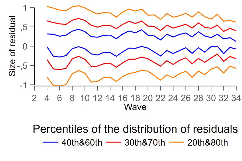
Figure 1 and Figure 2 are plots of the distribution of residuals that are used to construct the
instruments for income and life satisfaction.14 The plots underline the message of the Breusch-
Pagan test in Table A1.5. The distribution of the residuals of income narrows over the survey
years and respondents’ age. The distribution of the residuals of life satisfaction also narrows
11 For convenience age and squared survey wave are divided by 10, squared age and cubed wave are divided by
100, to avoid significant zeroes.
12 Reference income is the mean income of all individuals within an moving age range of 5 years younger and 5
years older, living in the same state (Bundesland), in households of the same size (top-coded at 5 persons per
household), and with similar highest level of education
13 Hospital overnight stay is not measured in the years 1990 and 1993. To avoid large data losses, I inserted
random numbers, generated from a binomial distribution with the the same success probability as the observed
variable.
14 Demeanded income and life satisfaction were regressed on demeaned exogenous controls, i.e. age, age2 , wave2
and wave3 .
10Table 1: Sample descriptives
Mean Std. Min Max
Dev.
Life satisfaction 7.009 1.733 0 10
Income 37587 18686 120 802920
Financial satisfaction 6.335 2.209 0 10
Age 41.641 10.812 20 60
Female 0.523 0.499 0 1
Years of education 12.047 2.680 7 18
Hospital overnight stay 0.102 0.303 0 1
Gave birth 0.015 0.121 0 1
Married 0.476 0.499 0 1
Children in household 0.662 0.473 0 1
Living in East Germany 0.199 0.399 0 1
Unemployed 0.067 0.250 0 1
Home owner 0.484 0.500 0 1
Source: SOEP v34, own calculations. 273,768 person year observations of
38134 individuals.
Notes: Hospital overnight stay for 261,782 person year observations, and
11986 imputed random numbers. Income is post-government household
income, not equivalized.
11Figure 1: Age- and wave-related heteroscedasticity in income
Source: SOEP v34, own calculations. 337031 person year observations of 46945 individuals.
Notes: Residuals from fixed effects regressions of income on age, age2 , wave2 and wave3
12Figure 2: Age- and wave-related heteroscedasticity in life satisfaction
Source: SOEP v34, own calculations. 337031 person year observations of 46945 individuals.
Notes: Residuals from fixed effects regressions of life satisfaction on age, age2 , wave2 and wave3
13Table 2: Squared residuals of endogenous regressors and exogenous controls
ν21it ν22it
(Equiv. income) (Life satisfaction)
Age –0.017*** –0.169***
(0.000) (0.007)
Age, sq. 0.010*** 0.099***
(0.000) (0.008)
Wave, sq. –0.005*** –0.083***
(0.000) (0.004)
Wave, cub. 0.001*** 0.016***
(0.000) (0.001)
Constant 0.135*** 2.783***
(0.001) (0.028)
Chi squared 4630 2087
Prob> Chi squared 0.000 0.000
Source: SOEP v34, own calculations. 337031 person year observations of
46945 individuals.
Notes: Significance levels * 0.10 ** 0.05 *** 0.01. Cluster-robust standard
errors in parentheses. Dependent variables are squared residuals from fixed
effects regressions, exogenous variables are within transformed.
over the survey years and reveals a slight tendency to narrow in the respondents’ middle ages.
Heteroskedasticity in financial satisfaction follows a similar pattern, the plots thereon are pre-
sented in the appendix in Figure A1.3. It thus appears as though the exogenous controls and
squared residuals are sufficiently associated to allow for identification based on Lewbel’s in-
struments.
5 Results
Results are presented in the same order as the model equations are discussed. Some notes apply
to all results: To avoid problems of weak instruments, I follow Baum et al. (2007), who suggest
the rule of thumb of Staiger and Stock (1997). This means that only estimates with F-statistics
> 10 should be trusted. Since the estimations rely on multiple observations per person, the
Wald F- statistics based on the reduced rank test of Kleibergen and Paap (2006) are valid test
statistics, because they are robust to non-i.i.d. errors. These F values are displayed as "K-P
F-Statistic" for each IV estimation in the bottom of the tables. Test statistics for the Hansen J
14test of overidentifying restrictions, which tests the null that the instruments are exogeous, are
reported under each IV estimation.15 In the bottom line of most estimation tables a z-score is
reported, which, when it’s absolute value exceeds 1.96, indicates that the estimates from the IV
procedure significantly differ from the conventional fixed effects estimates.
The complete estimation results are to be found in the appendix A1.1.
5.1 RQ1: Income causing satisfaction
The answer to RQ1 is provided in Table 3, and it obviously depends on the method. The conven-
tional fixed effects estimation confirms that increasing incomes are associated with increased
life satisfaction with a reasonable effect size. The estimates from the IV approach, however,
show no effect of income on life satisfaction.
Table 3: FE-IV and FE estimations of RQ1: Utility of equivalized household income
I II
IV-FE FE IV-FE FE
Income, log. 0.051 0.355*** –0.006 0.367***
(0.073) (0.013) (0.108) (0.015)
Demographic no no yes yes
controls
K-P F-Statistic 267 172
Hansen J 5.545 5.983
Prob>Chi sq. 0.1360 0.1125
Z-score –4.102 –3.408
Source: SOEP v34, own calculations. 273,768 person year observations of 38,134
individuals.
Notes: Significance levels * 0.10 ** 0.05 *** 0.01. Cluster-robust standard errors in
parentheses. All estimations include age, age2 , survey wave 2 and survey wave3 .
The most standard fixed effects regression result is presented in the last column of Table 3.
This is a fixed effects estimation of the association between income and life satisfaction, when
adding a large set of demographic controls (including health and marital status, education, (un-
)employment, region of residence, children, home ownership and reference income). This spec-
ification is thus closer to previous studies. The penultimate column shows results from the com-
parable estimation, where the same demographic control variables are included, but the internal
15 For the Hansen J test, it is thus a successfull result if χ2 indicates that the null is not rejected.
15instrumental variables approach is used. The instruments are exclusively constructed from the
exogenous controls (age, age squared and survey wave squared and cubed), but not from the
demographic controls. First and second column present results from the most sparse models,
with only age and wave (and its powers); where in the first column identification comes from the
internal instruments and in the second column the corresponding straightforward fixed effects
estimates are presented.
In general, the patterns in the estimations with and without further controls are similar:
The effects found through IV-estimations are zero while the FE-estimates are significantly pos-
itive. The z-sores indicate that the estimates from the two identification strategies differ signif-
icantly. Including further demographic controls does not meaningfully change the estimates:
even though the sign reverses, the IV estimates are statistically insignificant with and without
further demographic controls, the z-score to compare these coefficients is 0.437 (not given in
the table), indicating that the difference between the estimates is not statistically significant.
The conventional fixed effects estimates with and without further demographic controls are also
not significantly different from each other. This similarity in the patterns suggests that the exo-
geneity assumption (i.e. that the product of first and second stage errors is uncorrelated to the
exogenous controls) is not seriously violated due to omitted variables - at least not due to omit-
ting the demographic controls that were considered here. The Hansen J test, which is associated
with a p-value of more than 0.1 underlines this by also suggesting no violations to exogeneity.
5.2 RQ2: Satisfaction causing income
The preceding results showed that usual fixed effects estimations may overstate the effect of
income on life satisfaction. One possible reason for this finding could be reverse causality: life
satisfaction might cause income, as asked in RQ2.
Estimates in Table 4 support this hypothesis only weakly. Higher life satisfaction might
cause higher equivalized income, but significance is only weak and disappears when further
control variables are included in the estimation. Again, the coefficients of the conventional
fixed effects estimations are significantly positive. These, however, may be biased due to any
of the reasons mentioned in Section 3.1.
16Table 4: FE-IV and FE estimations of RQ2: Life satisfaction causing household income
I II
IV-FE FE IV-FE FE
Life satisfaction 0.011* 0.016*** 0.010 0.014***
(0.006) (0.001) (0.006) (0.001)
Demographic no no yes yes
controls
K-P F-Statistic 158 158
Hansen J 2.663 0.745
Prob>Chi sq. 0.4466 0.8626
Z-score –0.741 –0.723
Source: SOEP v34, own calculations. 273,768 person year observations of 38,134
individuals.
Notes: Significance levels * 0.10 ** 0.05 *** 0.01. Cluster-robust standard errors in
parentheses. All estimations include age, age2 , survey wave 2 and survey wave3 .
Covariates16 again, do not significantly change the results for the conventional fixed effects
estimates, and change only the significance test for the IV-FE estimation. According to the
test statistics, the IV estimation is trustworthy; Instruments are not weak and the model is not
misspecified, which could be interpreted as all instruments being exogenous.
The weak indication for a causal effect from life satisfaction on income matches the results
for RQ1 that higher incomes do not cause greater life satisfaction although the association
is significantly positive. The conventional fixed effects estimator could overstate the hedonic
effect of income due to reverse causality.
5.3 Re-estimation with satisfaction and income reported in the same
survey year
When thinking about mechanisms, it is reasonable to require that the effect should not precede
the cause; in the case of simultaneous causality between income and life satisfaction, this means
that both should refer to the same period. Thus, the analysis so far has focused on reported
16 The set of demographic covariates in the estimations for RQ2 is the same as for RQ1 except for giving birth
and reference income, these are not included in the estimations for Table 4.
17income, which refers to the year before the survey, and satisfaction from the previous survey
year.
In most estimates of the link between income and satisfaction, however, the income mea-
sure very often refers to the year prior to data collection and satisfaction statement. Although
effects of satisfaction on previous year’s income seem nonsensical at first glance, simultaneous
causality in this temporal order (of income and satisfaction data) is of particular interest because
it would limit the interpretation of most estimates. At second glance, and taking into account
that income is reported rather than measured, it seems possible that satisfaction at the time of
the survey could influence reported income in the year before the survey, e.g., through response
behavior.
Therefore, I re-estimate the models with satisfaction in the year of the survey and income in
the year before the survey.
Table 5: FE-IV and FE estimations of RQ1: Income in t-1 causing life satisfaction in t
I II
IV-FE FE IV-FE FE
Income, log. 0,104 0,373*** –0,015 0,342***
(0,074) (0,013) (0,109) (0,015)
Demographic no no yes yes
controls
K-P F-Statistic 267 172
Hansen J 18,22 18,12
Prob>Chi sq. 0,0004 0,0004
Z-score -3,5871 -3,242
Source: SOEP v34, own calculations. 273,768 person year observations of 38,134
individuals.
Notes: Significance levels * 0.10 ** 0.05 *** 0.01. Cluster-robust standard errors in
parentheses. All estimations include age, age2 , survey wave 2 and survey wave3 .
18Table 6: FE-IV and FE estimations of RQ2: life satisfaction in t causing income in t-1
I II
IV-FE FE IV-FE FE
Life satisfaction 0,027*** 0,017*** 0,023*** 0,015***
(0,007) (0,001) (0,007) (0,001)
Demographic no no yes yes
controls
K-P F-Statistic 112 113
Hansen J 7,061 3,797
Prob>Chi sq. 0,0700 0,2842
Z-score 1,4198 1,1228
Source: SOEP v34, own calculations. 273,768 person year observations of 38,134
individuals.
Notes: Significance levels * 0.10 ** 0.05 *** 0.01. Cluster-robust standard errors in
parentheses. All estimations include age, age2 , survey wave 2 and survey wave3 .
Results in Table 5 again do not indicate a causal effect of income on life satisfaction. Here,
income refers to the year before the survey and satisfaction at the time of the survey. Since
Hansen’s J is significantly above zero, the null of exogeneity of all included variables must
be rejected, i.e. the exogenous variables or the instruments or both do not meet the exogeneity
assumption. Estimates on RQ2, however, indicate a causal effect of satisfaction on income. The
IV estimates are similar in size and significance to the standard FE estimates. Together with the
previous results, this suggests that satisfaction could influence how respondents report their
income. Effects of satisfaction on equivalized income itself, whether through earning income
or sharing income, cannot appear in the temporal order analyzed in this estimation and would
likely be more pronounced after a period of more than one year.
This interpretation is supported by results from estimates in a third temporal order, where
again satisfaction and income are not reported in the same survey, but refer to the same year.
Satisfaction reported in the survey year t and income reported for the same year, but reported
in survey year t+1. The results are very similar to the main models with no significant effect of
income on life satisfaction and weak effects of life satisfaction on income. Results are presented
in the appendix in Tables A1.3 and A1.4
195.4 Robustness check with simulated data
One objection against the presented estimates might result from the fact that three of four IV
estimations reveal only small or zero and insignificant effects, while the corresponding conven-
tional fixed effects estimator found larger and significant effects. One might therefore suspect
that the Lewbel IV estimator is not suitable for either the discrete scale of the satisfaction data or
not capable of detecting small significant effects due to the reduced power which is common in
IV estimations and even more so when only within variation of the data is used. To address this
concern the same regressions are rerun on simulated data. On top of the SOEP data, I simulated
a random variable with panel data structure and a similar distribution as reported income.17
Table 7: Re-estimations of H1 and H2: For simulated random income and manipulated satis-
faction depending on simulated income
RQ1 RQ2
IV FE FE IV FE FE
Sim.Income 0.218*** 0.238***
(0.076) (0.026)
Sim.Satisf. 0.004 0.003***
(0.004) (0.000)
K-P F-Statistic 266 158
Hansen J 1.4 8.8
Prob>Chi sq. 0.7132 0.0325
Z-score –0.252 0.279
Source: SOEP v34, own calculations. 273,768 person year observations of 38,134
individuals.
Notes: Significance levels * 0.10 ** 0.05 *** 0.01. Cluster-robust standard errors in
parentheses. All estimations include age, age2 , survey wave 2 and survey wave3 .
I then manipulated the satisfaction data such that it depended on the simulated income data,
but preserved its scaling and distribution. This yields a simulated income measure, which is
completely exogenous, but correlated within individuals over time. I then manipulated the
satisfaction data such that it depends on the simulated income data, but preserves its scaling and
distribution. 18
17 Stata program code for the simulated income data is given in appendix A1.4.
18 Stata program code for the manipulated satisfaction data is given in appendix A1.4.
20This procedure results in a simulated income measure, which is completely exogenous, un-
correlated between individuals but correlated within, and satisfaction data that to some extent
depend on this exogenous simulated income. Hence in a re-estimation of RQ1 and RQ2 one
would expect that the conventional fixed effects estimator finds positive effects in both direc-
tions and that the IV-FE estimator finds only a positive effect for RQ1, i.e. the effect of simulated
income on manipulated satisfaction.
Results of re-estimations of H1 and H2 in Table 7 show the expected pattern, supported
by statistical tests. This may increase confidence that the zero effects presented in Sections 5
indeed represent the nonexistence of causal effects in the link between income and satisfaction
in the underlying population.
6 Conclusion
This study intended to explore simultaneity in the income-happiness link and to what extent this
might bias standard estimates of the hedonic effect of income. In that sense this study is method-
ological, since it does not focus the precise mechanisms that could generate the simultaneity.
Conclusions are both promising and disappointing.
They are disappointing because using Lewbel instruments, no significant causal effect from
income on life satisfaction is found, but instead indication for a causal effect of life satisfaction
on income. The zero effect of equivalized income on life satisfaction is unexpected and in
contradiction to most findings in this area of research. Nevertheless, one can be cautiously
optimistic that the zero effects are not a problem due to the estimator or its application, for two
reasons: First, most studies in this field do not properly identify causal effects, but estimate
merely associations under consideration of covariates and individual level fixed effects. Among
those studies that use convincing methods, results indicate that long-term changes in income
have significant and sizable effects on life satisfaction (Vendrik 2013, Bayer and Juessen 2015)
while short-term shocks do not influence life satisfaction (Bayer and Juessen 2015, Lachowska
2017). Second, in a simulation, where satisfaction data was manipulated so that it depends on a
simulated random, but income-like variable, the estimator found the simulated effect.
Results on the second research question indicate that life satisfaction indeed influences the
measure for equivalized household income. This effect is statistically significant when income
21and satisfaction data are collected in the same survey year, but only weakly significant when
income data is reported in another survey year but refers to the same year as the satisfaction
data. This pattern of reverse causality is likely due to response behavior rather than income
generation. In conclusion, it must be considered that the effect of income on life satisfaction is
probably overstated in conventional fixed effects estimations.
The present analysis is promising because Lewbel’s (2012) internal instruments passed the
tests for weak instruments in each specification. This is encouraging news for empirical sat-
isfaction research, as this method might be able to solve the problem focused on here and fill
a gap that still exists in empirical happiness research: Identifying causal effects between life
satisfaction and its correlates.
22References
Baetschmann, G., Staub, K. E., and Winkelmann, R. (2015). Consistent estimation of the fixed
effects ordered logit model. Journal of the Royal Statistical Society A, 178(3):685–703.
Baum, C. and Lewbel, A. (2019). Advice on using heteroskedasticity-based identification. Stata
Journal, 19(4):757–767.
Baum, C. F. and Schaffer, M. E. (2012). IVREG2H: Stata module to perform instrumental
variables estimation using heteroskedasticity-based instruments. Statistical Software Com-
ponents, Boston College Department of Economics.
Baum, C. F., Schaffer, M. E., and Stillmand, S. (2007). Enhanced routines for instrumental
variables/generalized method of moments estimation and testing. Stata Journal, 7(4):465–
506.
Bayer, C. and Juessen, F. (2015). Happiness and the persistence of income shocks. American
Economic Journal: Macroeconomics, 7(4):160–187.
Böckerman, P. and Ilmakunnas, P. (2012). The job satisfaction-productivity nexus: A study
using matched survey and register data. ILR Review, 65(2):244–262.
Boyce, C. J., Brown, G. D. A., and Moore, S. C. (2010). Money and happiness: Rank of income,
not income, affects life satisfaction. Psychological Science, 21(4):471–475.
Boyce, C. J., Daly, M., Hounkpatin, H. O., and Wood, A. M. (2017). Money may buy happiness,
but often so little that it doesn’t matter. Psychological Science, 28(4):544–546.
Brown, S. and Gray, D. (2016). Household finances and well-being in Australia: An empirical
analysis of comparison effects. Journal of Economic Psychology, 53:17–36.
Bryson, A., Forth, J., and Stokes, L. (2017). Does employees’ subjective well-being affect
workplace performance? Human Relations, 70(8):1017–1037.
Bubonya, M., Cobb-Clark, D. A., and Wooden, M. (2017). Mental health and productivity at
work: Does what you do matter? Labour Economics, 46:150–165.
Bütikofer, A. and Gerfin, M. (2017). The economies of scale of living together and how they
are shared: Estimates based on a collective household model. Review of Economics of the
Household, 15(2).
Carver, T. and Grimes, A. (2019). Income or consumption: Which better predicts subjective
well-being? Review of Income and Wealth, 65(S1).
Clark, A. E., Frijters, P., and Shields, M. A. (2008). Relative income, happiness, and utility: An
explanation for the easterlin paradox. Journal of Economic Literature, 46:95–144.
D’Ambrosio, C. and Frick, J. R. (2012). Individual wellbeing in a dynamic perspective. Eco-
nomica, 79(314):284–302.
23De Neve, J.-E., Diener, E., Tay, L., and Xuereb, C. (2013). The objective benefits of subjective
well-being. In Helliwell, J., Layard, R., and Sachs, J., editors, World Happiness Report 2013,
pages 1–35. UN Sustainable Development Solutions Network.
De Neve, J.-E. and Oswald, A. J. (2012). Estimating the influence of life satisfaction and posi-
tive affect on later income using sibling fixed effects. Proceedings of the National Academy
of Sciences, 109(49):19953–19958.
Diener, E. and Oishi, S. (2000). Money and happiness: Income and subjective well being
across nations. In Diener, E. and Suh, E., editors, Subjective Well-being Across Cultures,
pages 185–218. MIT Press, Cambridge MA.
Easterlin, R. (1974). Does economic growth improve the human lot? Some empirical evidence.
In David, P. and Reder, M., editors, Nations and Households in Economic Growth: Essays in
Honor of Moses Abramovitz, pages 89–125. Academic Press.
Easterlin, R. A. (1995). Will raising the incomes of all increase the happiness of all? Journal
of Economic Behavior & Organization, 27(1):35–47.
Easterlin, R. A. (2005). Feeding the illusion of growth and happiness: A reply to Hagerty and
Veenhoven. Social Indicators Research, 74(3):429–443.
Easterlin, R. A. (2017). Paradox lost? Review of Behavioral Economics, 4(4):311–339.
Elsas, S. (2021). Satisfaction as an outcome, as a means and as a cause.
Elsas, S. E. (2016). Income sharing within households: Evidence from data on financial satis-
faction. Social Sciences, 5(47).
Frey, B. S. and Stutzer, A. (2002). What can economists learn from happiness research? Journal
of Economic Literature, 40(2):402–435.
Frick, J. R., Goebel, J., Schechtman, E., Wagner, G. G., and Yitzhaki, S. (2006). Using anal-
ysis of Gini (AnoGi) for detecting whether two sub-samples represent the same universe:
The German Socio-Economic Panel Study (SOEP) experience. Sociological Methods & Re-
search, 34(4):427–468.
Frijters, P., Haisken-DeNew, J. P., and Shields, M. A. (2004). Money does matter! evidence
from increasing real income and life satisfaction in east germany following reunification.
American Economic Review, 94(3):730–740.
Frijters, P., Johnston, D. W., Shields, M. A., and Sinha, K. (2015). A lifecycle perspective of
stock market performance and wellbeing. Journal of Economic Behavior & Organization,
112:237–250.
Goebel, J., Grabka, M. M., Liebig, S., Kroh, M., Richter, D., Schröder, C., and Schupp, J.
(2019). The german socio-economic panel study (soep). Jahrbücher für Nationalökonomie
und Statistik / Journal of Economics and Statistics, 239(2):345–360.
Graham, C., Eggers, A., and Sukhtankar, S. (2004). Does happiness pay? In Glatzer, W.,
Von Below, S., and Stoffregen, M., editors, Challenges for Quality of Life in the Contempo-
rary World, volume 24 of Social Indicators Research Series, pages 179–204. Springer.
24Guardiola, J. and Guillen-Royo, M. (2015). Income, unemployment, higher education and
wellbeing in times of economic crisis: Evidence from Granada (Spain). Social Indicators
Research, 120(2):395–409.
Guven, C. (2012). Reversing the question: Does happiness affect consumption and savings
behavior? Journal Economic Psychology, 33(4):62–78.
Hagenaars, A. J. M., de Vos, K., and Asghar Zaidi, M. (1994). Poverty statistics in the late
1980s: Research based on microdata. Official publications of the European Communities,
Eurostat (European Commission), Luxembourg.
Hagerty, M. R. and Veenhoven, R. (2003). Wealth and happiness revisited: Growing national
income does go with greater happiness. Social Indicators Research, 64(1):1–27.
Jäntti, M., Kanbur, R., Nyyssölä, M., and Pirttilä, J. (2014). Poverty and welfare measurement
on the basis of prospect theory. Review of Income and Wealth, 60(1):182–205.
Kahneman, D. and Deaton, A. (2010). High income improves evaluation of life but not emo-
tional well-being. Proceedings of the National Academy of Sciences, 107(38):16489–16493.
Kaiser, C. (2018). People do not adapt to income changes: A re-evaluation of the dynamic
effects of (reference) income on life satisfaction with gsoep and ukhls data. MPRA Papers,
89867.
Kaiser, C. and Vendrik, M. C. (2019). Different versions of the easterlin paradox: New evidence
for european countries. In Rojas, M., editor, The Economics of Happiness, pages 27–55.
Springer.
Kesavayuth, D. and Zikos, V. (2018). Happy people are less likely to be unemployed: Psycho-
logical evidence from panel data. Contemporary Economic Policy, 36(2):277–291.
Kleibergen, F. and Paap, R. (2006). Generalized reduced rank tests using the singular value
decomposition. Journal of Econometrics, 133(1):97–126.
Knight, J., Song, L., and Gunatilaka, R. (2009). Subjective well-being and its determinants in
rural china. China Economic Review, 20(4):635–649.
Krause, A. (2013). Don’t worry, be happy? Happiness and reemployment. Journal of Economic
Behavior & Organization, 96(C):1–20.
Lachowska, M. (2017). The effect of income on subjective well-being: Evidence from the 2008
economic stimulus tax rebates. Journal of Human Resources, 52(2):374–417.
Lane, T. (2017). How does happiness relate to economic behaviour? A review of the literature.
Journal of Behavioral and Experimental Economics, 68:62–78.
Layard, R., Mayraz, G., and Nickell, S. J. (2008). The marginal utility of income. Journal of
Public Economics, 92(8-9):1846–1857.
Lewbel, A. (2012). Using heteroscedasticity to identify and estimate mismeasured and endoge-
nous regressor models. Journal of Business & Economic Statistics, 30(1):67–80.
25Luttmer, E. (2005). Neighbours as negatives: relative earnings and well-being. Quarterly
Journal of Economics, 120(3):963–1002.
Mishra, V. and Smyth, R. (2014). It pays to be happy (if you are a man): Subjective wellbeing
and the gender wage gap in urban China. International Journal of Manpower, 35(3):392–414.
Ng, W. and Diener, E. (2014). What matters to the rich and the poor? Subjective well-being,
financial satisfaction, and postmaterialist needs across the world. Journal of Personality and
Social Psychology, 107(2):326–338.
OECD (2008). Growing unequal? Income distribution and poverty in OECD countries. Official
publications of the oecd, Organisation for Economic Co-operation and Development, Paris.
OECD (2011). Divided we stand–why inequality keeps rising. Official publications of the
OECD, Organisation for Economic Co-operation and Development, Paris.
Oswald, A. J. (1997). Happiness and economic performance. The Economic Journal,
107(445):1815–1831.
Oswald, A. J., Proto, E., and Sgroi, D. (2015). Happiness and productivity. Journal of Labor
Economics, 33(4):789–822.
Powdthavee, N. (2010). How much does money really matter? Estimating the causal effects of
income on happiness. Empirical Economics, 39(1):77–92.
Schnitzlein, D. D. and Wunder, C. (2016). Are we architects of our own happiness? The
importance of family background for well-being. The B.E. Journal of Economic Analysis &
Policy, 16(1):125–149.
Schwarze, J. (2003). Using panel data on income satisfaction to estimate equivalence scale
elasticity. Review of Income and Wealth, 49(3):359–372.
Staiger, D. and Stock, J. H. (1997). Instrumental variables regression with weak instruments.
Econometrica, 65(3):557–586.
Stevenson, B. and Wolfers, J. (2008). Economic growth and subjective well-being: Reassessing
the easterlin paradox. Brookings Papers on Economic Activity, 39(1):1–102.
Stutzer, A. (2004). The role of income aspirations in individual happiness. Journal of Economic
Behavior & Organization, 54(1):89–109.
Tenney, E. R., Poole, J. M., and Diener, E. (2016). Does positivity enhance work performance?:
Why, when, and what we don’t know. Research in Organizational Behavior, 36:27–46.
Vendrik, M. (2013). Adaptation, anticipation and social interaction in happiness: An integrated
error-correction approach. Journal of Public Economics, 105:131–149.
Vendrik, M. and Woltjer, G. (2007). Happiness and loss aversion: Is utility concave or convex
in relative income? Journal of Public Economics, 91(7-8):1423–1448.
Walsh, L. C., Boehm, J. K., and Lyubomirsky, S. (2018). Does happiness promote career
success? Revisiting the evidence. Journal of Career Assessment, 26(2):199–219.
26You can also read