Modeling Australian TEC Maps Using Long-Term Observations of Australian Regional GPS Network by Artificial Neural Network-Aided Spherical Cap ...
←
→
Page content transcription
If your browser does not render page correctly, please read the page content below
remote sensing
Article
Modeling Australian TEC Maps Using Long-Term
Observations of Australian Regional GPS Network by
Artificial Neural Network-Aided Spherical Cap
Harmonic Analysis Approach
Wang Li 1,2 , Dongsheng Zhao 1 , Yi Shen 3 and Kefei Zhang 1,2, *
 1    School of Environmental Science and Spatial Informatics, China University of Mining and Technology,
      Xuzhou 221116, China; liwang@cumt.edu.cn (W.L.); dszhao@cumt.edu.cn (D.Z.)
 2    SPACE Research Center, School of Science, RMIT University, Melbourne, VIC 3001, Australia
 3    Key Laboratory for Synergistic Prevention of Water and Soil Environmental Pollution,
      Xinyang Normal University, Xinyang 464000, China; shenyi@xynu.edu.cn
 *    Correspondence: profkzhang@cumt.edu.cn

 Received: 18 October 2020; Accepted: 21 November 2020; Published: 24 November 2020

 Abstract: The global ionosphere map (GIM) is not capable of serving precise positioning and
 navigation for single frequency receivers in Australia due to sparse International GNSS Service (IGS)
 stations located in the vast land. This study proposes an approach to represent Australian total
 electron content (TEC) using the spherical cap harmonic analysis (SCHA) and artificial neural network
 (ANN). The new Australian TEC maps are released with an interval of 15 min for longitude and
 latitude in 0.5◦ × 0.5◦ . The validation results show that the Australian Ionospheric Maps (AIMs) well
 represent the hourly and seasonally ionospheric electrodynamic features over the Australian continent;
 the accuracy of the AIMs improves remarkably compared to the GIM and the model built only by the
 SCHA. The residual of the AIM is inversely proportional to the level of solar radiation. During the
 equinoxes and solstices in a solar minimum year, the residuals are 2.16, 1.57, 1.68, and 1.98 total
 electron content units (TECUs, 1 TECU = 1016 electron/m2 ), respectively. Furthermore, the AIM has a
 strong capability in capturing the adequate electrodynamic evolutions of the traveling ionospheric
 disturbances under severe geomagnetic storms. The results demonstrate that the ANN-aided SCHA
 method is an effective approach for mapping and investigating the TEC maps over Australia.

 Keywords: Australian ionospheric model; spherical cap harmonic analysis; artificial neural network;
 Australian regional GNSS network; geomagnetic storm

1. Introduction
     It is well known that the ionospheric delay effect is one of the major error sources for global
navigation satellite system (GNSS) radio signal propagation. The ionosphere is a dispersive medium
for the radio signal, the direction of the radio signal is refracted when the GNSS signal propagates
in the dispersive medium. The delay error is proportional to the total electron content (TEC) that is
the total number of free electrons along the signal propagation path from the satellite to the receiver,
and it is function of the carrier frequency of the signal [1]. Therefore, the delay error of GNSS signals
caused by ionospheric refraction can be removed once the TEC is determined. For dual-frequency
or multi-frequency receivers, the TEC quantity can be estimated by the ranging observations of the
pseudo-range and carrier phase. While, for the single-frequency receiver, the TEC value predicted by a
TEC model is usually as an alternative method for mitigating the ionospheric refraction. Based on
coverage, TEC models can be divided into global and regional models. Now the famous global TEC

Remote Sens. 2020, 12, 3851; doi:10.3390/rs12233851                        www.mdpi.com/journal/remotesensing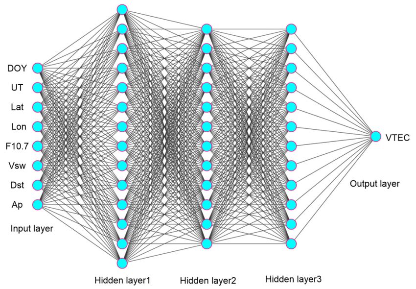
Remote Sens. 2020, 12, 3851                                                                      2 of 20

models contain NeQuick [2], Klobuchar [3], Bent [4], international reference ionosphere (IRI) [5], etc.
The NeQuick and improved Klobuchar have been successfully applied in the space missions of Great
Britain, Australia, the United States, and China. The Ionosphere Associate Analysis Centers (IAACs)
of the International GNSS Service (IGS) began to release reliable global ionospheric maps (GIMs) since
1998, the maps are estimated by the spherical harmonics using dual-frequency observations of about
400 GPS/GLONASS sites of the IGS and other institutions. With the growing demands of high-accuracy
GNSS services, the traditional global ionospheric models with low spatial-temporal resolutions cannot
meet the requirement for regional applications [6]. In this condition, some regional TEC models with
higher mapping accuracy are developed using the observations derived from regional dense GNSS
stations. A spherical cap harmonic model was developed with a data set from 40 GNSS stations
for mapping and predicting TEC in China [7], this model not only maps regional TEC values with
higher accuracy but also has a powerful capability in predicting ionospheric variations based on
spectrum analysis and least-squares collocation. The validation demonstrates that the spherical cap
harmonic analysis (SCHA)-based TEC model has a remarkable advantage rather than the conventional
polynomial model and GIM, and this method has been applied widely in modeling regional ionosphere
over Canada, the Arctic area, Iran, Japan, Antarctica [8–12]. The obtained results further confirm the
usefulness of the SCHA method for building near-real-time regional maps as well as its expanding
potential application in other ionospheric parameters modeling.
     Australia is comprised of the mainland of the Australian continent, the island of Tasmania,
and numerous smaller islands. It is also a composite of diverse landscapes, the surrounding coastal
regions are flatland and mountain land, and the central areas of Australia are desert and grassland.
Most citizens live in some big cities, such as Sydney, Melbourne, Adelaide, Brisbane, etc. The stations
of the Australian Region GPS Network (ARGN) mainly distribute in the coastal regions, while few
stations are located in the center of Australia. Because the GNSS observations over the central region
of Australia is insufficient, the equations are easy to fall into “ill-condition” problem when using
the dual-frequency observations of the ARGN to develop the Australia TEC model by the SCHA
method. Therefore, it is necessary to capture more virtual TEC information over the “no-station” areas
of Australia to solve the “ill-condition” problem.
     The artificial neural network is a computing system designed to replicate the way humans analyze
and work, which is good at studying the complex relationship between one physical parameter
and various independent factors [13]. It is well known that various competing dynamical and
electrodynamical processes control the ionospheric behavior [14–16], such as the disturbance dynamo
electric fields, the prompt penetration electric fields, and the interaction between ions and neutrals.
The ANN technique has a main advantage in capturing the nonlinear relationships between the
ionospherical physical parameters and various solar-terrestrial factors, compared to many other
techniques used in modeling ionospheric maps, such as the empirical orthogonal function (EOF)
decomposition technique [17], principal component analysis [18] and support vector machine [19].
The ANN technique has proven to be a successful tool in the ionospheric modeling for various
parameters as well as solving the forecast problems in many geophysical applications over a single
station, regional area, and global scale [20–24].
     In this study, an artificial neural network (ANN)-based Australian TEC model is developed to
predict the TEC values over the area that lacks observations firstly, then both the observations of
the ARGN and the predicted TEC values are utilized to build an Australia TEC model by the SCHA
method. The structure of the present paper is organized as follows. The ARGN network and the
data preparation process are introduced in Section 2.1. The adopted methodologies including the
SCHA method and the ANN technique are described in Section 2.2. The accuracies and ionospheric
electrodynamic features of the Australian TEC maps under various levels of solar radiations are
validated in Section 3. Additionally, the responses of the Australian TEC maps to severe geomagnetic
storms on 22 June 2015, are investigated and compared to the global ionosphere maps in Section 4.
Finally, the merits of this model along with its future improvements are discussed in Section 5.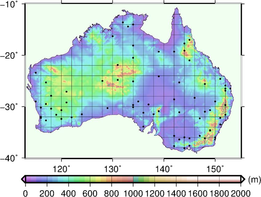
which point the ARGN could provide the 30s-resolution dual or multiple frequency observations of
more than 200 GNSS stations. The stations of the ARGN are shown in Figure 1. In this study, the
dual-frequency measurements provided by the ARGN with a data set of 2006–2017 are used to
construct the Australian ionospheric TEC maps, the observations can be downloaded from
ftp://ftp.ga.gov.au/geodesy-outgoing/gnss.
Remote Sens. 2020, 12, 3851                         It is must be noted that few observations are obtained      3 of 20
from the GNSS stations located at Tasmania island, hence in this study, the scope of the Australian
TEC maps is only limited within mainland Australia.
2. Materials and Methods
      According to the theory of ionospheric delay effect, the TEC value can be obtained from a
difference
2.1. Materialsof delay between the two radio waves [25]. Therefore, in this study, the dual-frequency
observation files should be checked for quality control by the translation, editing, and quality
      The Australian
checking     (TEQC) softwareregional
                                   in GPS  network
                                      the initial      (ARGN)
                                                  stage.          was constructed
                                                           The TEQC     software is from      the 1990s
                                                                                      developed     by a until  2017,
                                                                                                          non-profit
at which   point    the  ARGN    could  provide  the  30s-resolution   dual or  multiple
university-governed consortium, facilitates geoscience research and education using geodesyfrequency   observations
of more thanit200
(UNAVCO),           is aGNSS
                         simplestations.  The stations
                                 yet powerful  and unifiedof the
                                                              toolARGN    are shown
                                                                   in solving          in Figure 1. Inproblems
                                                                               many pre-processing       this study, of
the  dual-frequency       measurements     provided     by the  ARGN     with  a data  set
GNSS observations obtained from multiple navigation systems including GPS, GLONASS, Galileo,of  2006–2017   are used
to constructSBAS,
Beidou,          the Australian
                            QZSS, ionospheric
                                      and         TEC maps,
                                             IRNSS.        The the TEQCobservations
                                                                              softwarecan be is downloaded
                                                                                                   obtained from from
ftp://ftp.ga.gov.au/geodesy-outgoing/gnss.          It is must be noted thatInfew
https://www.unavco.org/software/data-processing/teqc/teqc.html.                   theobservations
                                                                                        quality controlare stage,
                                                                                                            obtained
                                                                                                                   the
from   the GNSS      stations  located at Tasmania    island,  hence  in this study, the  scope   of
observations with the multi-path noises (MP1, MP2) of exceed 0.8 as well as the cycle slips of exceedthe Australian
TEC   maps
300 are       is only limited within mainland Australia.
          removed.

     Figure1.1.Geographic
     Figure     Geographic     distribution
                            distribution      ofstations
                                         of the  the stations   of the Australian
                                                         of the Australian          Regional
                                                                           Regional GPS      GPSthe
                                                                                        Network,  Network,  the
                                                                                                    background
     background   map   is the digital
     map is the digital elevation map. elevation   map.

      According
2.2. Artificial   to theNetwork-Based
                Neural   theory of ionospheric delay
                                       Australian TECeffect,
                                                       Model the TEC value can be obtained from a difference
of delay between the two radio waves [25]. Therefore, in this study, the dual-frequency observation
      The artificial neural network (ANN) technique is a promising tool in capturing the nonlinear
files should be checked for quality control by the translation, editing, and quality checking (TEQC)
relationships between multiple variables, and is formed by large numbers of simple processing
software in the initial stage. The TEQC software is developed by a non-profit university-governed
elements known as neurons. This technique has been widely applied in ionospheric modeling, data
consortium, facilitates geoscience research and education using geodesy (UNAVCO), it is a simple yet
classification, image recognition, etc. [26]. Backpropagation (BP) is one of the most successful
powerful and unified tool in solving many pre-processing problems of GNSS observations obtained
algorithms in the ANN training process, which consists of two stages: feed-forward and back-
from multiple navigation systems including GPS, GLONASS, Galileo, Beidou, SBAS, QZSS, and IRNSS.
forward. In a feed-forward process, the input datasets are studied by the ANN technique to generate
The TEQC software is obtained from https://www.unavco.org/software/data-processing/teqc/teqc.html.
In the quality control stage, the observations with the multi-path noises (MP1, MP2) of exceed 0.8 as
well as the cycle slips of exceed 300 are removed.

2.2. Artificial Neural Network-Based Australian TEC Model
      The artificial neural network (ANN) technique is a promising tool in capturing the nonlinear
relationships between multiple variables, and is formed by large numbers of simple processing elements
known as neurons. This technique has been widely applied in ionospheric modeling, data classification,
image recognition, etc. [26]. Backpropagation (BP) is one of the most successful algorithms in the ANN
training process, which consists of two stages: feed-forward and back-forward. In a feed-forward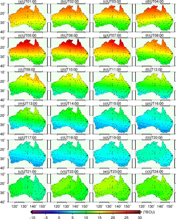
Remote Sens. 2020, 12, 3851 4 of 20
Remote Sens. 2020, 12, x FOR PEER REVIEW 4 of 20
process, the input datasets are studied by the ANN technique to generate predicted values, and the
predicted
predictederrors
values,are
andcomputed by the
the predicted difference
errors betweenbytarget
are computed values and
the difference predicted
between values.
target valuesIn
anda
back-forward
predicted values. process,
In a the predicted errors
back-forward are the
process, transferred
predicted from theare
errors output layer tofrom
transferred the input layer,
the output
and
layerthen theinput
to the inputlayer,
weights
andare adjusted.
then the inputIn weights
this study,
areaadjusted.
simple BP In neural network
this study, formed
a simple by an
BP neural
input
networklayer, three by
formed hidden layers,
an input andthree
layer, an output
hidden layer is utilized
layers, and anto develop
output layeranisAustralian
utilized toTEC model.
develop an
AAustralian
dataset consists of dayA
TEC model. ofdataset
year (DOY), universal
consists of day time (UT),
of year geographic
(DOY), latitude
universal time(Lat),
(UT),geographic
geographic
longitude (Lon),
latitude (Lat), F10.7 cm solar
geographic flux (F10.7),
longitude (Lon), solar
F10.7 wind speed
cm solar flux(Vsw), Dst,solar
(F10.7), and wind
Ap is speed
selected as input
(Vsw), Dst,
parameters. The vertical
and Ap is selected as inputtotal electron content
parameters. (VTEC)
The vertical totalvalues
electron incontent
the output
(VTEC)layer are estimated
values by
in the output
the dual-frequency
layer are estimatedGNSS observation
by the of the ARGN
dual-frequency GNSS using pseudo-range
observation observation
of the ARGN usingsmoothed with
pseudo-range
carrier phasesmoothed
observation [27]. Thousands of experiments
with carrier are conducted
phase [27]. Thousands to search the
of experiments areoptimal
conducted combination of
to search the
neural
optimal neurons in threeofhidden
combination neurallayers. Theinresults
neurons three indicate
hidden that the The
layers. root-mean-square
results indicate error
that(RMSE) is
the root-
minimum
mean-square when the(RMSE)
error numbersisof neurons when
minimum are 14,the12,numbers
12 in three ofhidden
neuronslayers,
are 14,and12,the corresponding
12 in three hidden
active
layers,functions in three hiddenactive
and the corresponding layersfunctions
are tansig,intansig, and sigmod,
three hidden layersrespectively. The architecture
are tansig, tansig, and sigmod,of
the ANN-based
respectively. TheAustralian TECofmodel
architecture is shown inAustralian
the ANN-based Figure 2. TEC model is shown in Figure 2.
Figure2.2.Architecture
Figure Architectureof
ofthe
theANN-based
ANN-basedAustralia
Australiatotal
totalelectron
electroncontent
content(TEC)
(TEC)model.
model.
2.3.
2.3.ANN-Aided
ANN-AidedSCHA
SCHAApproach
Approachfor
forAustralian
AustralianVTEC
VTECModeling
Modeling
Ionospheric
Ionospheric TECTEC maps
mapsreleased
releasedby bythe
theInternational
InternationalGNSS
GNSSServices
Services(IGS)
(IGS)have
havedemonstrated
demonstrated
that
that the spherical harmonics analysis is very suitable to develop ionospheric models on a global
the spherical harmonics analysis is very suitable to develop ionospheric models on a global scale.
scale.
However,
However, the Legendre polynomial expansion in spherical harmonics is difficult to map theTEC
the Legendre polynomial expansion in spherical harmonics is difficult to map the TECover
over
aaregional area, the regional area is called as “cap”. The spherical cap harmonic analysis is
regional area, the regional area is called as “cap”. The spherical cap harmonic analysis is availableavailable to
develop a cap model well using the spherical cap coordinate system, and the spherical
to develop a cap model well using the spherical cap coordinate system, and the spherical cap cap harmonic
parameters can derive by
harmonic parameters cansolving
derive abyLaplace’s
solving equation over
a Laplace’s a specific
equation spherical
over cap.spherical
a specific This method has
cap. This
been
methodsuccessfully
has beenapplied to regional
successfully appliedTEC models [7].
to regional TEC models [7].
The
The zenith VTEC over a specific sphericalcap
zenith VTEC over a specific spherical capcan
canbebeexpressed
expressedas:as:
kX k k k
max max
θ ξ P m m ⋅ ξ ))
mnk ( m ) (cos θ )( Ak ⋅mcos( m ⋅ ξ ) + Bk ⋅ sin(
X m m m
VTEC ( , ) =
VTEC(θ, ξ) = P ( cos θ )( A · cos ( m·ξ ) + B · sin ( m·ξ )) (1)
(1)
k = 0 m = 0 n (m)
k k k
k =0 m=0
where (θ, ξ) is the coordinate of the ionospheric pierce point (IPP) in spherical cap coordinate, kmax
where (θ, ξ) is the coordinate of the ionospheric pierce point m(IPP) in spherical cap coordinate, kmax is
is the maximum order, in this study kmax is set as 8. Pnk ( m ) (cos θ ) is the normalized associated
the maximum order, in this study kmax is set as 8. Pm nk ( m )
(cos θ) is the normalized associated Legendre
m m
Legendre
function function
where n andwhere
n (m)nare
k
and n (
integral
k m)
andare integral
real degrees, and real degrees,
respectively. and Bm are theAnormalized
Am respectively. k and Bk
k k
are the normalized spherical cap harmonic coefficients. For more details about the spherical cap
harmonic theory please refer to [27,28].
Remote Sens. 2020, 12, 3851 5 of 20
spherical cap harmonic coefficients. For more details about the spherical cap harmonic theory please
refer to [27,28].
In this study, the Australian TEC maps can be estimated by the spherical cap harmonic method
with the following steps:
(1) The slant TEC along the path from a satellite to a receiver is estimated by the dual-frequency
observations using pseudo-ranges smoothed with carrier phases, and the hardware differential
code biases (DCB) of GNSS satellites and receivers are also corrected, please refer to [29]. The TEC
in any epoch can be computed by the linear combination of pseudo-ranges and carrier phases
as follows:
f12 f22 f12 f22
TECp,k = ( P2 − P1 ) + (Bp,r + Bsp ) (2)
40.28( f12 − f22 ) 40.28( f12 − f22 )
− f12 f22 f12 f22
TECφ,k = (λ2 φ2 − λ1 ]φ1 ) − (λ2 N2 − λ1 N1 + Bφ,r + Bsφ ) (3)
40.28( f12 − f22 ) 40.28( f12 − f22 )
where TECp,k and TECφ,k represent the TEC values derived from pseudo-range and carrier phase
observations at epoch k, respectively. The subscripts r and s indicate the receiver and satellite,
f 1 and f 2 are signal frequencies, Pi and φi are dual-frequency pseudo-range and carrier phase
observations. λ1 and λ2 are the wavelengths of carrier phase l1 and l2 , N1 and N2 are the
ambiguities of carrier phase measurements (l1 and l2 ). Bp,r and Bsp are the receiver and satellite
DCBs on the pseudo-range measurements, Bφ,r and Bsφ are the receiver and satellite DCBs on the
carrier phase measurements. Usually, the receiver and satellites DCBs are regarded as stable in a
few days [30], then
∆TECk = TECp,k − TECφ,k =
f12 f22
40.28( f12 − f22 )
(Bp,r + Bsp + λ2 N2 − λ1 N1 + Bφ,r + Bsφ ) (4)
f2 f2
+ 40.28(1 f 22− f 2 ) (P2 − P1 + λ2 φ2 − λ1 φ1 )
1 2
Generally, the ∆TECk is stable in a day, a more precise TEC observation can be computed by a
recursive smoothing process.
N
N−1
∼ 1X 1 X
∆TEC = ∆TECn = ∆TECn + ∆TECN (5)
N N
n=1 n=1
The smoothed ionospheric TEC calculates by:
∼ − f12 f22 ∼ f2 f2
∆TECk = (λ2 φ2 − λ1 φ1 ) + ∆TEC − 40.28(1 f 22− f 2 ) (Bp,r + Bsp ) =
40.28( f12 − f22 ) 1 2
− f12 f22 N f12 f22
f12 f22
2 2 ( λ2 φ2 − λ1 φ1 ) + N
1 P
2 2 ( P2 − P1 + λ2 φ2 − λ1 φ1 ) − (Bp,r + Bsp ) =
40.28( f − f ) 40.28( f − f ) 40.28( f12 − f22 )
1 2 n=1 1 2
N f2 f2 N−1 f2 f2 f12 f22
1 1
( 40.28(1 f 22− f 2 ) (λ2 φ2 − λ1 φ1 )) − (Bp,r + Bsp )
P
( 40.28(1 f 22− f 2 ) (P2 − P1 )) +
P
N N 40.28( f12 − f22 )
n=1 1 2 n=1 1 2
(6)
(2) Convert the slant TEC (STEC) to the vertical TEC (VTEC) at a pierce point using the single-layer
model function, the height of the single layer is set as 428.8 km.
(3) Predict the TEC time series over the central points of the blank grid in Figure 1 using the
ANN-based Australian TEC model, the blank grid means the regions where no experimental data
are available.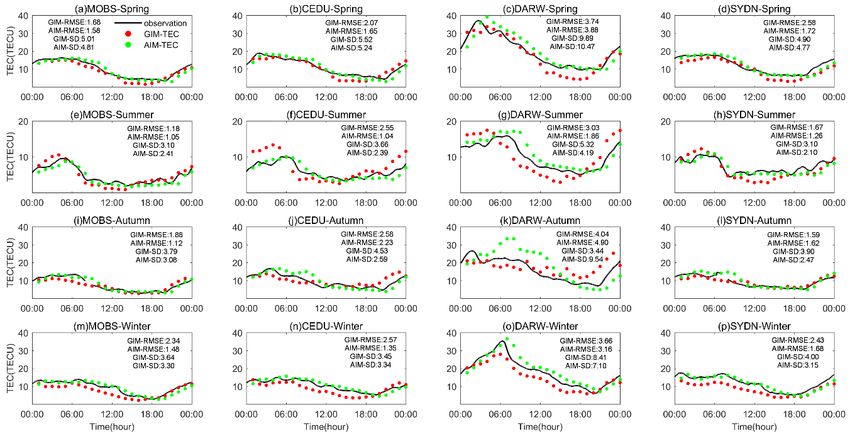
Remote Sens. 2020, 12, 3851                                                                                  6 of 20

(4)   Determine the pole point and the half-angle of the spherical cap to design the spherical cap
      coordinate system. According to the studying scope of the Australian map, the pole of the
      spherical cap is set as (−25◦ , 133◦ ), the half-angle is determined as 20◦ , and the maximum order is
      chosen as 8.
(5) Transform the coordinates of ionospheric pierce points and the central points of blank grids from
 Remote Sens. 2020, 12, x FOR PEER REVIEW                                                             6 of 20
      the geographic coordinate system to the spherical cap coordinate system, Figure 3 illustrates the
      transformation relationship between the spherical cap coordinate system and the geographic
      transformation relationship between the spherical cap coordinate system and the geographic
      coordinate system. If the geographic coordinates of the pole of the spherical cap are θP and
      coordinate system. If the geographic coordinates of the pole of the spherical cap are θP and λP,
      λP, then the spherical cap coordinate (θC, λC) of any point Q (θ, λ) can be calculated using the
      then the spherical cap coordinate (θC, λC) of any point Q (θ, λ) can be calculated using the
      following equations:
      following equations:
                          cos(θcos
                                c ) (= ) =(θcos
                                     θccos   P ) (cos(
                                                   θP ) θ       ) +θsin
                                                          ) +(θsin(
                                                        cos              θP ) θsin
                                                                     P )(sin(    ) cos( λ −(λλ−P )λP )
                                                                                   (θ) cos
                                                                                                                   (7)
                              tan(π − λ ) = sin(λ ) cossin( θ ) sin(λ − λP )(λ−λ )
                                                         sin(θ) sin(λ−λP )                                        (7)
                          tan(π − λc ) =c          P    (θ)−cos(θP ) sin(θ) cos P
                                         sin(λP ) cos(θ ) − cos(θ P ) sin(θ ) cos(λ − λP )
(6) Calculate the model coefficients (Am  , Bm ) in Equation (1) using the least square method, and verify
                                        k mk m
 (6) the
     Calculate  the model coefficients ( A  k , Bk ) cap
         performance of the estimated spherical       in Equation
                                                          model by(1) using thethe
                                                                   comparing     least square
                                                                                    model’s   method,TEC
                                                                                            predicted and
     verify the
     values     performance
             with           of the estimated
                  the TEC observations   at thespherical   cap model
                                                 pierce points of GNSSby stations.
                                                                         comparing the model’s predicted
     TEC values with the TEC observations at the pierce points of GNSS stations.

      Figure      Transformation relationship
      Figure 3.3. Transformation relationship between
                                              between geographic
                                                      geographic coordinate
                                                                 coordinate system
                                                                            system and
                                                                                   and spherical
                                                                                       spherical cap
                                                                                                 cap
      coordinate
      coordinatesystem.
                   system.

3. Results
3. Results
     In this study, an artificial neural network-aided spherical cap harmonic analysis approach is
      In this study, an artificial neural network-aided spherical cap harmonic analysis approach is
proposed to estimate the Australian ionospheric TEC maps using long-term dual-frequency observations
proposed to estimate the Australian ionospheric TEC maps using long-term dual-frequency
derived from the ARGN, the Australian ionospheric map is abbreviated as AIM. The Australian TEC
observations derived from the ARGN, the Australian ionospheric map is abbreviated as AIM. The
maps are released with an interval of 15 min for geographic longitude and latitude in 0.5◦ × 0.5◦ .
Australian TEC maps are released with an interval of 15 min for geographic longitude and latitude
in 0.5°
3.1.    × 0.5°. with the AIMSCHA Model in 2013 and 2017
     Comparison
     To evaluate with
3.1. Comparison    the efficiency  of the ANN
                         the AIMSCHA      Modeltechnique  in 2017
                                                in 2013 and  ionospheric modeling, the Australian TEC maps
are also estimated only using the spherical cap harmonic analysis, namely AIMSCHA . The performances
of theTo  evaluate
       AIMs          the efficiency
              are validated   in solarofmedium
                                         the ANN   technique
                                                year           in solar
                                                      (2013) and  ionospheric
                                                                        minimum  modeling,  the compared
                                                                                   year (2017)   AustraliantoTEC
                                                                                                              the
maps    are  also estimated     only   using the  spherical  cap  harmonic    analysis,  namely
AIMSCHA maps, the TEC time series derived from the dual-frequency measurements of the ARGN        AIM  SCHA. The

performances
stations         of theasAIMs
         are chosen             are validated
                          references.          in solar medium
                                        The comparative   results year  (2013) in
                                                                   are shown    and solar
                                                                                  Table 1. minimum year (2017)
compared to the AIMSCHA maps, the TEC time series derived from the dual-frequency measurements
of the ARGN stations are chosen as references. The comparative results are shown in Table 1.

      Table 1. Comparative results of the predicted root-mean-square errors (RMSEs) of the AIMSCHA and
      AIM maps in 2013 and 2017 (unit: TECU).

       Year                       2013 (Medium)                                       2017 (Minimum)
      Season        Spring      Summer Autumn Winter                    Spring       Summer Autumn       Winter
      AIMSCHA        3.76         2.68      2.82  3.84                   2.37          1.75      1.83     2.11
       AIM           3.41         2.42      2.54  3.65                   2.16          1.57      1.68     1.98
       Ratio        9.31%        9.70%     9.93% 4.95%                  8.86%        10.28%     8.20%    6.16%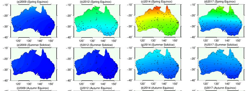
Remote Sens. 2020, 12, 3851                                                                          7 of 20

      Table 1. Comparative results of the predicted root-mean-square errors (RMSEs) of the AIMSCHA and
      AIM maps in 2013 and 2017 (unit: TECU).

             Year                2013 (Medium)                         2017 (Minimum)
           Season       Spring   Summer Autumn Winter        Spring    Summer Autumn Winter
          AIMSCHA         3.76    2.68     2.82      3.84      2.37     1.75       1.83      2.11
            AIM           3.41    2.42     2.54      3.65      2.16     1.57       1.68      1.98
           Ratio         9.31%   9.70%    9.93%     4.95%     8.86%    10.28%     8.20%     6.16%

     As shown in Table 1, both the predicted RMSEs of the AIMSCHA and AIM maps in the solar
minimum year are remarkably smaller than that in the solar medium year, and the RMSEs in summer
and autumn are much smaller than that in spring and winter. Compared to the AIMSCHA model,
the ANN technique could improve the predicted capability of the Australian TEC maps to a certain
degree. The ratio is calculated as (AIM − AIMSCHA )/AIMSCHA . For example, the predicted RMSEs
of the AIM maps in spring, summer, autumn, and winter of 2013 are 3.41, 2.42, 2.54, and 3.65 TECU,
which is about 9.31%, 9.70%, 9.93% and 4.95% smaller than the RMSEs of the AIMSCHA maps. This
conclusion is also suitable in 2017, the predicted accuracies of the AIM maps improve about 8.86%,
10.28%, 8.20% and 6.61% than the AIMSCHA maps in spring, summer, autumn, and winter, respectively.
The comparative results demonstrate that the ANN technique not only plays an important role in
solving the “ill condition” when estimating the spherical cap harmonic function, but also improves the
predicted accuracy of the AIM model with a degree of 8–10%, especially in high-level solar activities.

3.2. Seasonal and Hourly Features of the AIM Maps
      To further validate the spatial characteristics of the AIM maps dependent on the level of solar
radiation, the Australian TEC maps in different solar activity years 2009, 2012, 2014, and 2017 during
the 23–24 solar cycles are estimated by the dual-frequency observations derived from the ARGN.
The seasonal variations of the Australian TEC maps at the universal time (UT) 00:00 hour are shown in
Figure 4. In this figure, the black points represent the ARGN’s stations which observations have passed
the quality control stage. Figure 4a–d show that the GNSS stations of the ARGN network increasing
rapidly from 2009, and most of these stations locate in the coastal areas, such as New South Wales,
Victoria, Western Australia, etc. In Australia, the TEC value is inversely proportional to the geographic
latitude, the TEC value in northern Australia is about two-times larger than that in the southern area.
From 2009, with solar activity recovering to a normal level, the TEC value gradually increases and
reaches to the maximum in 2014. Seasonal variations of Australian ionospheric maps show the TEC
values in spring equinox and winter solstice are maximum, and in summer solstice the TEC value is
minimum, which is caused by the revolution of the earth. Additionally, during the years 2009–2012
with the rising phase of solar radiation in solar cycle 24, the TEC values in spring equinox are lower
than that in winter solstice; while the phenomenon is opposite in the declining phase (2014–2017) in
the solar cycle 24.
      Figure 5 shows the hourly variations of Australian TEC maps on the winter solstice of 2016.
From Figure 5a at UT01:00, the TEC in Australia gradually enhances and reaches a maximum value of
30 TECU at UT05:00 (Figure 5e). After that, it begins to decrease and reaches a minimum value of
5 TECU at UT20:00. The high TECs appear in the period of UT04:00 (Figure 5d) to UT07:00 (Figure 5g),
the corresponding local time (LT) is LT14:00 to LT17:00. The daytime TEC values over the northern
area of Australia are 2–3 times larger than that in other regions, and the TEC variations over this
region located at the south crest of the equatorial ionization anomaly are more violent. Figures 4 and 5
demonstrate that the Australian TEC maps estimated by the SCHA method optimized by the ANN
technique are consistent with the global ionospheric maps provided by the CODE [31], which indicates
that the AIM model is successful to capture the spatial-temporal characteristics of Australian TEC
variations well.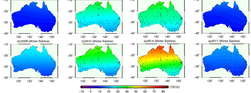
Remote Sens. 2020, 12, 3851                                                                                        8 of 20

3.3. Mapping Performance of the AIM Model under Quiet and Disturbed Geomagnetic Conditions

3.3.1. Validation of the Mapping Performance under Quiet Geomagnetic Condition
     The global ionosphere maps released by the IGS are estimated by the dual-frequency observations
of more than 400 GNSS stations. Among them, only about 10 stations located in Australia are
used. To evaluate the mapping accuracy of the AIM model under a quiet geomagnetic condition,
the vertical TEC time series over four GNSS stations that have been used to develop the GIM and
AIM models are selected as references. The names of four stations are MOBS (144.58◦ E, 37.49◦ S),
CEDU (133.48◦ E, 31.52◦ S), DARW (131.08◦ E, 12.50◦ S), and SYDN (151.09◦ E, 33.46◦ S). They are
distributed in Melbourne, Ceduna, Darwin, and Sydney, respectively. The predicted TEC values over
the four stations are extracted from the products of the GIM and AIM models, namely GIM–TEC and
AIM–TEC. The comparative results between true TEC, GIM–TEC, and AIM–TEC in the equinoxes and
solstices of 2016 are shown in Figure 6.
Remote Sens. 2020, 12, x FOR PEER REVIEW                                                                          8 of 20

      Figure 4.
      Figure 4. Spatial
                Spatial variations
                         variations of
                                    of the  Australian TEC
                                       the Australian          maps in
                                                          TEC maps   in the
                                                                        the equinoxes
                                                                            equinoxes and
                                                                                        and solstices,
                                                                                             solstices, the
                                                                                                        the time
                                                                                                            time of
                                                                                                                  of
      each subfigure
      each subfigureisisuniversal
                         universaltime
                                    time00:00.
                                           00:00.(a–d)
                                                   The show
                                                        each panels from theTEC
                                                             the Australian    topmaps
                                                                                    row to
                                                                                        in the bottom
                                                                                           spring        rowduring
                                                                                                   equinox    are in
      spring equinox,
      2009–2017, (e–h) summer
                        in summersolstice, autumn
                                    solstice, (i–l) inequinox
                                                       autumnand   winter(m–p)
                                                               equinox,    solstice duringsolstice.
                                                                                 in winter  years 2009, 2012, 2014
      and 2017

      Figure 5 shows the hourly variations of Australian TEC maps on the winter solstice of 2016.
From Figure 5a at UT01:00, the TEC in Australia gradually enhances and reaches a maximum value
of 30 TECU at UT05:00 (Figure 5e). After that, it begins to decrease and reaches a minimum value of
5 TECU at UT20:00. The high TECs appear in the period of UT04:00 (Figure 5d) to UT07:00 (Figure
5g), the corresponding local time (LT) is LT14:00 to LT17:00. The daytime TEC values over the
northern area of Australia are 2–3 times larger than that in other regions, and the TEC variations over
this region located at the south crest of the equatorial ionization anomaly are more violent. Figures 4
and 5 demonstrate that the Australian TEC maps estimated by the SCHA method optimized by the
ANN technique are consistent with the global ionospheric maps provided by the CODE [31], which
indicates that the AIM model is successful to capture the spatial-temporal characteristics of
Australian TEC variations well.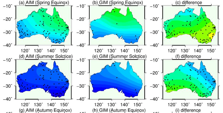
Remote Sens. 2020, 12, 3851                                                                            9 of 20
Remote Sens. 2020, 12, x FOR PEER REVIEW                                                             9 of 20

       Figure 5. Hourly Australian TEC maps predicted by the AIM model on the winter solstice in 2016.
      Figure 5. Hourly Australian TEC maps predicted by the AIM model on the winter solstice in 2016,
      (a–x) show the temporal variations of Australian TEC maps from UT01:00 to UT24:00 with an interval
3.3. Mapping Performance of the AIM Model under Quiet and Disturbed Geomagnetic Conditions
      of one hour.

3.3.1. Validation of the Mapping Performance under Quiet Geomagnetic Condition
     The global ionosphere maps released by the IGS are estimated by the dual-frequency
observations of more than 400 GNSS stations. Among them, only about 10 stations located in
Australia are used. To evaluate the mapping accuracy of the AIM model under a quiet geomagnetic
condition, the vertical TEC time series over four GNSS stations that have been used to develop the
GIM and AIM models are selected as references. The names of four stations are MOBS (144.58° E,
37.49° S), CEDU (133.48° E, 31.52° S), DARW (131.08° E,12.50° S), and SYDN (151.09° E, 33.46° S).
They are distributed in Melbourne, Ceduna, Darwin, and Sydney, respectively. The predicted TEC
values over the four stations are extracted from the products of the GIM and AIM models, namely
Remote Sens. 2020, 12, x FOR PEER REVIEW 10 of 20
GIM–TEC
Remote and12,
Sens. 2020, AIM–TEC.
3851 The comparative results between true TEC, GIM–TEC, and AIM–TEC in
10 of 20
the equinoxes and solstices of 2016 are shown in Figure 6.
Figure 6. Comparative
Figure 6. Comparative results
results of
of the
the performances
performances of of the
the GIM
GIM and
and AIM
AIM over Stations MOBS, CEDU,
DARW,
DARW,and andSYDN
SYDNin in2016,
2016,the
thered
redand
andgreen
greenlines
linesindicate
indicatethe
theGIM
GIMand
andAIM
AIMtime
timeseries,
series,(a–d) show
the panels
the comparative results over Stations MOBS, CEDU, DARW, and SYDN in spring equinox,
from the top row to the bottom row are in spring equinox, summer solstice, autumn equinox and (e–h) in
summer solstice, (i–l) in autumn equinox, (m–p) in winter solstice.
winter solstice.
Generally,
Generally,the theGIM–TEC
GIM–TECand andAIM–TEC
AIM–TEC values
values agree
agree well with
well withthethetruetrueTECTEC timetime
series, bothboth
series, the
TEC maps
the TEC mapssuccess
successto reproduce
to reproduce thethehourly
hourlydynamic
dynamic features
featuresofofionospheric
ionosphericelectron electroncontent
content over over
Australia.
Australia. However, the RMSE and standard deviation (SD) of the AIM–TEC are smaller than
However, the RMSE and standard deviation (SD) of the AIM–TEC are smaller than thethe
GIM–TEC,
GIM–TEC, and and thethe RMSEs
RMSEs and and SDs
SDs ofof the
the AIM
AIM model
model are are dependent
dependent on on thethe season
season and and geographic
geographic
latitude
latitude remarkably.
remarkably.For Forthe
the season,
season, thethe accuracies
accuraciesof of the
the AIM
AIM model
model in in summer
summer solstice
solstice andand autumn
autumn
equinox are highest, followed by winter solstice, while spring equinox
equinox are highest, followed by winter solstice, while spring equinox is lowest. The phenomenon is is lowest. The phenomenon
is caused
caused byby thethe level
level of seasonal
of seasonal solarsolar radiation
radiation in 2016.
in 2016. From From
FigureFigure
6e–h, it 6e–h, it is that
is found found thethatRMSEsthe
RMSEs of the TEC time series extracted from the AIMs over station
of the TEC time series extracted from the AIMs over station MOBS, CEDU, DARW, and SYDN are MOBS, CEDU, DARW, and SYDN
are 1.05,
1.05, 1.04,1.04,
1.86,1.86,
1.261.26
TECU, TECU, respectively.
respectively. The The corresponding
corresponding RMSEs RMSEsof TEC of TEC
time time
seriesseries
derived derived
from
from the GIMs
the GIMs over four overstations
four stations
are 1.18,are 1.18,
2.55, 2.55,
3.03, and3.03,
1.67andTECU. 1.67ForTECU.
SDs, the Forindices
SDs, the indices
of the AIMs ofover
the
AIMs over station MOBS, CEDU, DARW, and SYDN are 2.41, 2.39,
station MOBS, CEDU, DARW, and SYDN are 2.41, 2.39, 4.19, and 2.10 TECU, respectively, and the 4.19, and 2.10 TECU, respectively,
and the corresponding
corresponding SDs forSDs theforGIMs
the GIMs are 3.10,
are 3.10, 3.66,3.66,
5.32,5.32,
and and 3.10TECU.
3.10 TECU.The The comparative
comparative results results
demonstrate that the Australian TEC maps estimated by the SCHA
demonstrate that the Australian TEC maps estimated by the SCHA method with ANN-aided method with ANN-aided technique
are superiorare
technique to the GIMs to
superior remarkably,
the GIMsand the accuracies
remarkably, and the (RMSEs) of the (RMSEs)
accuracies AIM improve of the about
AIM11%, 59%,
improve
38.6%
about and
11%,25% 59%,over38.6% theand
above25%stations
over the compared to the compared
above stations GIMs. Besides, to thethe mapping
GIMs. Besides,performance
the mapping of
the AIM model has a close relationship with the geographic latitude.
performance of the AIM model has a close relationship with the geographic latitude. For example, For example, the RMSE of station
DARW
the RMSE located in the northern
of station area of Australia
DARW located is maximum,
in the northern area oftheAustralia
averagedispredicted
maximum, residual exceeds
the averaged
3predicted
TECU, and the maximum
residual exceeds 3 SD TECU,exceeds
and the10 TECU.
maximum Station DARW 10
SD exceeds is located
TECU. Stationat the southern
DARW iscrest locatedof
equatorial ionization anomaly (EIA), where the equatorial ionosphere is
at the southern crest of equatorial ionization anomaly (EIA), where the equatorial ionosphere is veryvery violent that controlled by
the fountain
violent thateffect [32], equatorial
controlled by theeastward
fountainelectric
effectfield
[32],[33],equatorial
thermospheric eastwardparticleelectric
exchange [34],[33],
field etc.
The mapping performance of the AIM model over the station MOBS
thermospheric particle exchange [34], etc. The mapping performance of the AIM model over the is best, which station is located in
the southern area of Australia. The predicted RMSEs in four seasons (Figure
station MOBS is best, which station is located in the southern area of Australia. The predicted RMSEs 6a,e,i,m) are 1.58, 1.05,
1.12, and 1.48
in four TECU,
seasons respectively,
(Figure andare
6a,e,i,m) the improvements
1.58, 1.05, 1.12, rangeandfrom1.485%TECU,
to 40% compared
respectively, to the and GIMs.
the
Furthermore, it is noted that sometimes the performance of the AIM
improvements range from 5% to 40% compared to the GIMs. Furthermore, it is noted that sometimes model is worse than the GIM
over the equatorial
the performance ofstation.
the AIM For example,
model in Figure
is worse than 6c,k,
the GIM the predicted RMSEs and
over the equatorial SDs ofFor
station. theexample,
AIM for
station
in FigureDARW6c,k,are thelarger than RMSEs
predicted the GIMand during
SDsspring
of the and
AIMautumn.
for station ThisDARW
limitation shouldthan
are larger be improved
the GIM
in futurespring
during work.and autumn. This limitation should be improved in future work.
Figure
Figure 11 shows
shows the the number
number of of ARGN
ARGN stations
stations used
used forfor developing
developing the the AIM
AIM mapsmaps is is much
much largerlarger
than
than the IGS stations located in Australia. To further validate the mapping performance of the AIM
the IGS stations located in Australia. To further validate the mapping performance of the AIMRemote Sens. 2020, 12, 3851 11 of 20
Remote Sens. 2020, 12, x FOR PEER REVIEW 11 of 20
maps
mapsoveroverthe
theblank
blankgridgridwhere
whereno noIGS
IGSobservations
observationsareareavailable,
available,the theTEC
TECvalues
valuesestimated
estimatedby bythe
the
dual-frequency measurements of ARGN stations while do not belong to the
dual-frequency measurements of ARGN stations while do not belong to the IGS network are selected IGS network are selected
as ◦ ◦ ◦
asthe
thereference.
reference. The
The details
details of
of two
two stations
stations are
areMRO1
MRO1 (116.38
(116.38° E, E, 26.41
26.41° S)S) and
and MCHL
MCHL (148.08
(148.08° E, E,
26.21 ◦ S). The comparative results between the AIM–TEC and GIM–TEC are shown in Figure 7.
26.21° S). The comparative results between the AIM–TEC and GIM–TEC are shown in Figure 7. From
From the panels
the panels of theofleftthe left column,
column, the RMSEs the RMSEs of the AIM–TEC
of the AIM–TEC over MRO1
over station stationat MRO1 at theequinox,
the spring spring
equinox,
summer summer solstice,equinox,
solstice, autumn autumn and equinox,
winterand winter
solstice aresolstice are1.87,
2.26, 1.68, 2.26,and
1.68, 1.87,
1.66 and respectively,
TECU, 1.66 TECU,
respectively, the mapping accuracies improve about 25.41%, 60.47%, 54.83%,
the mapping accuracies improve about 25.41%, 60.47%, 54.83%, and 44.30% compared to the GIMs. and 44.30% compared to
the
TheGIMs.
SDs of ThetheSDs of the
AIMs AIMs
are alsoare also 16.61%,
16.61%, 38.39%,38.39%,
27.25%,27.25%, and 0.002%
and 0.002% smallersmaller
thanthan the GIMs
the GIMs at
at the
the corresponding equinoxes and solstices. For the station MCHL, the mapping
corresponding equinoxes and solstices. For the station MCHL, the mapping performances of the performances of the
AIM–TEC
AIM–TECduring duringfour
fourseasons
seasonsimprove
improvebybyaboutabout46.31%,
46.31%,25.29%,
25.29%, 47.22%,
47.22%, and and37.08%.
37.08%. Figures
Figures 6 and
6 and7
demonstrate
7 demonstrate thethe
AIMAIM model
model has
has a more
a more powerful
powerfulcapability
capabilityininreproducing
reproducingthe thehigh-accuracy
high-accuracyTEC TEC
maps over the entire Australian continent.
maps over the entire Australian continent.
Figure 7. Similar to Figure 7. Similar
Figure to Figure
6, but for 6, MRO1
stations but for stations
and MCHL,MRO1 and MCHL.
(a,c,e,g) show the comparative
results over station MRO1 in spring equinox, summer solstice, autumn equinox and winter solstice,
The relationship
(b,d,f,h) over stationbetween
MCHL. the mapping residual of the AIM model and the level of solar activity
is investigated in Figure 8. In this study, the averaged RMSEs of the GNSS stations of the ARGN on
The relationship
the equinoxes betweenduring
and solstices the mapping residual
2012–2017 of the AIMitmodel
are calculated, andthat
is found the level of solar
the RMSE of activity
the ANN- is
investigated in Figure 8. In this study, the averaged RMSEs of the GNSS stations
TEC in June (Figure 8b) is minimum with an average mapping residual of 2 TECU. The RMSEs in of the ARGN on the
equinoxes and solstices
March (Figure during 2012–2017
8a) and December areare
(Figure 8d) calculated,
maximum it is found
with that the residual
an average RMSE ofofthe 3 toANN-TEC
3.5 TECU.
in June (Figure
Besides, 8b) isvalues
the RMSE minimum withinwith
theanperiod
average mapping residual (about
of UT04:00–UT12:00 of 2 TECU. The RMSEs inare
LT14:00–LT22:00) March
two-
(Figure 8a) and December (Figure 8d) are maximum with an average residual of
times larger than that in other hours, which is due to the high-level solar radiation and the3 to 3.5 TECU. Besides,
the RMSE values
ionospheric within the
scintillations periodwith
related of UT04:00–UT12:00
the low-latitudinal(about
plasma LT14:00–LT22:00) are two-times larger
bubbles after sunset.
than that in other hours, which is due to the high-level solar radiation and the ionospheric scintillations
related with the low-latitudinal plasma bubbles after sunset.Remote Sens. 2020, 12, 3851 12 of 20
Remote Sens. 2020, 12, x FOR PEER REVIEW 12 of 20
Figure 8.
Figure 8. Mapping
Mapping performances
performances ofof the
the AIM
AIM maps
maps during
during 2012–2017,
2012–2017, the
the RMSEs
RMSEs of
of AIM–TEC
AIM–TEC maps
maps
are computed
are computed in in (a)
(a) spring
spring equinox,
equinox, (b)
(b) summer
summer solstice,
solstice, (c)
(c) autumn
autumn equinox
equinox and
and (d)
(d) winter
winter solstice,
solstice,
respectively, (e)
respectively, (e) shows
showsthetheF10.7
F10.7solar
solarflux
fluxtime
timeseries
seriesduring
during2012–2018.
2012–2018.
Figure 8e shows
showsthe thelevel
levelofofsolar
solarradiation
radiation enhances
enhances from 2012
from andand
2012 reaches a peak
reaches in 2014,
a peak and
in 2014,
thenthen
and the the
solar activity
solar gradually
activity gradually declines.
declines.Meanwhile,
Meanwhile, thethemapping
mappingresiduals
residualsofofthe
the AIM model
during 2013–2014 is significantly larger than that in the years 2016–2017. For example, in Figure 8d,
the averaged RMSE of the AIM model during 2013–2014 is 3.5 TECU, which is 1.5 TECU larger than
the mapping residuals at 2016–2017. 2016–2017. The results demonstrate that the mapping performance of the
AIM model
AIM model hashas aa close
close relationship
relationship withwith the
the level
level of
of solar
solar radiation,
radiation, and
and this
this model
model might
might achieve
achieve
better performance under under quiet
quiet solar
solar conditions.
conditions.
The above
The abovesections
sectionsshowshowthat
thatthethe
AIMAIM model
model developed
developed by SCHA
by the the SCHA method
method with with the ANN-
the ANN-aided
aided technique
technique could successfully
could successfully generategenerate the high-accuracy
the high-accuracy AustralianAustralian
TEC map. TEC map. investigate
To further To further
investigate
the the spatial differences
spatial differences between the between the Australian
Australian TEC mapsTEC mapsfrom
derived derived
thefrom
GIMthe andGIM
AIM and AIM
model,
model,
the middaythe and
midday and midnight
midnight TEC mapsTEC on themaps on theand
equinoxes equinoxes
solsticesand solstices
in 2016 in 2016 are
are computed. computed.
From Figure 9,
From
it Figure
is found 9, it
that is spatial
the found that the spatial
features of the features
AIM–TEC of maps
the AIM–TEC
agree wellmaps
withagree well with
the GIMs, but the
the GIMs,
GIMs
but the
seem toGIMs
hold seem
a leadtoofhold a lead
several of several
phases overphases overmaps.
the AIM’s the AIM’sFrommaps. From the
the panels of panels of the
the right right
column,
column,
the the TECextracted
TEC values values extracted
from thefromAIMsthe areAIMs
largerare larger
than the than
GIMsthe GIMs
over over Western
Western Australia,Australia,
but this
but this phenomenon
phenomenon is oppositeis opposite overAustralia.
over eastern eastern Australia. The difference
The positive positive difference
is maximum is maximum on the
on the summer
summerwith
solstice solstice with a magnitude
a magnitude of 8 TECUofat8 Western
TECU atAustralia,
Western Australia, and the maximum
and the maximum negative
negative difference
difference
covers covers the Queensland
the Queensland with a magnitude
with a magnitude of −6 TECUofduring
−6 TECU theduring
winter the winter solstice.
solstice.Remote Sens. 2020, 12, 3851 13 of 20
Remote Sens. 2020, 12, x FOR PEER REVIEW 13 of 20
Figure
Figure 9.
9. Spatial
Spatial differences
differences between
between the
the Australian
Australian TEC
TEC maps
maps mapped
mapped by by the
the AIM
AIM and
and GIM
GIM at
at local
local
time
time 12:00,
12:00, 11 January
January 2016,
2016, the
the black
panelspoints
of therepresent
left and middle columns
the GNSS represent
stations, theshow
(a,d,g,j) TEC the
maps derived
TEC maps
from thefrom
derived AIMthe andAIM
GIMmodel
model, in the black
spring points summer
equinox, representsolstice,
the GNSS stations.
autumn equinox and winter solstice,
(b,e,h,k) show the TEC maps derived from the GIM model, (c,f,i,l) show the differences between the
Figure
TEC maps 10 shows
derivedthe
fromspatial
the AIMdifferences
and GIM. between the Australian TEC maps derived from the AIM
and GIM at midnight. Generally, the spatial feature of the AIM map is consistent with the GIM map
well,Figure
and the10difference
shows thebetween
spatial differences
the two kinds between theat
of maps Australian
midnightTEC maps than
is smaller derived
thatfrom the AIM
at noon. The
and GIM
panels at midnight.
in the right columnGenerally,
show thatthe spatial feature of
the differences inthe
theAIMspringmap is consistent
equinox (Figurewith
10c)the
andGIM map
summer
well,
solsticeand the difference
(Figure between the
10f) are minimum, andtwothekinds of mapsranges
magnitude at midnight
from −3is to smaller
3 TECU.thanOn that
theatwinter
noon.
The panels
solstice in the 10l),
(Figure right the
column show that
AIM–TEC mapsthe differences
are smallerinthanthe spring equinox
the GIMs over(Figure 10c) and
the entire summer
Australian
solstice (Figure
continent, and the 10f) are minimum,
remarkable negativeanddifferences
the magnitudecoverranges from −3
the northern andtosoutheast
3 TECU. Australia
On the winter
with
asolstice (Figure
magnitude of10l), the AIM–TEC
exceeds –4 TECU.maps are smaller
Especially on thethan the GIMs
autumn over(Figure
equinox the entire Australian
10i), the TEC continent,
values of
and AIM
the the remarkable negative differences
maps are remarkably larger than cover theGIMs
the northern
overand southeast Australia
central-eastern with
Australia, a magnitude
the maximum
of exceeds –4 TECU. Especially on the autumn equinox (Figure 10i),
amplitude reaches to 8 TECU. The remarkable TEC differences between the AIM and GIM maps the TEC values of the AIM maps
are
are remarkably
believed larger than
to be caused the GIMs
by different over
time central-eastern
resolutions. SinceAustralia, the maximum
2015, the CODE releasedamplitude reaches
a new version of
to 8 TECU.
global TECThe mapremarkable TEC differences
with a one-hour interval, between
while in the
thisAIM
study andtheGIM
timemaps are believed
resolution of thetoAustralian
be caused
by different
TEC map based timeonresolutions.
the SCHA Since
method 2015, themin.
is 15 CODEThereleased
AIM map a new
has anversion of global
averaged 30-min TEC mapdelay
phase with
a one-hourtointerval,
compared the GIM. while in this study
The midday the time
ionospheric resolution
variation of theby
affected Australian
the strongTEC solarmap based is
radiation onvery
the
SCHA method
violent, therefore is 15
themin. The spatial
midday AIM map has an averaged
differences between 30-min
the twophase
models delay compared
are more to the GIM.
remarkable than
that at midnight.Remote Sens. 2020, 12, 3851 14 of 20
The midday ionospheric variation affected by the strong solar radiation is very violent, therefore the
midday spatial differences between the two models are more remarkable than that at midnight.
Remote Sens. 2020, 12, x FOR PEER REVIEW 14 of 20
Figure 9,
Figure 10. Similar to Figure 10.but
Similar to Figure
at midnight, 9, but at2016,
1 January midnight, 1 January
(a,d,g,j) 2016.
show the TEC maps derived from
the AIM model in spring equinox, summer solstice, autumn equinox and winter solstice, (b,e,h,k) show
3.3.2. Validation of the Mapping Performance under the Severe Geomagnetic Condition
the TEC maps derived from the GIM model, (c,f,i,l) show the differences between the TEC maps
Section
derived 3.3.1
from thedemonstrates
AIM and GIM.that the AIM model has a good mapping performance under quiet
geomagnetic conditions. In this section, we will further investigate the mapping performance of the
3.3.2.
AIMValidation of the
model under Mapping
a severe Performance
geomagnetic under
storm. Thethe Severe
severe Geomagnetic
geomagnetic stormCondition
on 22 June 2015, is
selected as 3.3.1
Section a casedemonstrates
study, and the response
that the AIMof the AIMhas
model maps to this
a good geomagnetic
mapping storm is under
performance analyzed.
quiet
The variation of the GIM map within the period of the violent storm is also investigated
geomagnetic conditions. In this section, we will further investigate the mapping performance of for
thecomparison.
AIM modelThis geomagnetic
under storm started storm.
a severe geomagnetic from UT19:00, June geomagnetic
The severe 22, and reached the most
storm on 22violent at
June 2015,
UT04:30,as
is selected June 23 with
a case study,a maximum of Dst value
and the response of theofAIM
−207nT.
mapsThe geomagnetic
to this condition
geomagnetic stormonis 21 June
analyzed.
2015, was quiet, hence the TEC values on the day are utilized as reference values. The TEC responses
The variation of the GIM map within the period of the violent storm is also investigated for comparison.
of the AIM and GIM to the geomagnetic event are shown in Figures 11 and 12, respectively.
This geomagnetic storm started from UT19:00, June 22, and reached the most violent at UT04:30,
June 23 with a maximum of Dst value of −207nT. The geomagnetic condition on 21 June 2015, was quiet,
hence the TEC values on the day are utilized as reference values. The TEC responses of the AIM and
GIM to the geomagnetic event are shown in Figures 11 and 12, respectively.Remote Sens. 2020, 12, 3851 15 of 20
Remote Sens. 2020, 12, x FOR PEER REVIEW 15 of 20
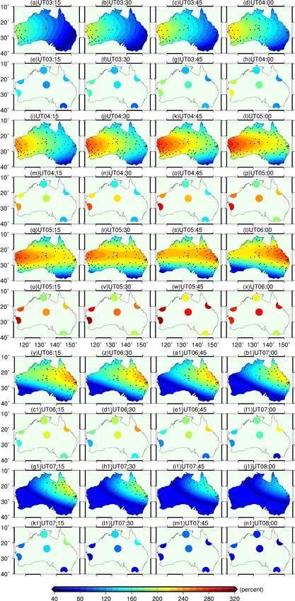
Figure 11. TEC responses of the AIM map during the main phase of the severe geomagnetic storm on
Figure 11. TEC responses of the AIM map during the main phase of the severe geomagnetic storm on
23 June 2015, the time interval is 15 min, the dots indicate the TEC perturbations of the referenced IGS
23 June 2015, the time interval is 15 min, the dots indicate the TEC perturbations of the referenced IGS
stations, (a–n1) show the magnitude of Australian TEC enhancements derived from the AIM maps
during UT03:15–UT08:00 with an interval of 15 minutes.Remote Sens. 2020, 12, x FOR PEER REVIEW 16 of 20
Remotestations,
Sens. 2020, 12, 3851
(a–n1) 16 of 20
show the magnitude of Australian TEC enhancements derived from the AIM maps
during UT03:15–UT08:00.
Figure
Figure 12.
12. TEC
TEC responses
responses of
of the
the GIM
GIM map
map during
during the
the main
main phase
phase of
of the
the severe
severe geomagnetic
geomagnetic storm
storm on
on
23 June 2015, the time interval is 15 min, (a–l) show the magnitude of Australian TEC enhancements
23 June 2015, the time interval is 15 min, (a–l) show the magnitude of Australian TEC enhancements
derived
derived from the GIM
from the GIM maps
maps during
during UT03:00–UT08:00
UT03:00–UT08:00.with an interval of one hour.
In Figure 11, the maps represent the Australian TEC responses of the AIM map to the severe
geomagnetic
geomagnetic storm, storm, andand thethe dots
dots represent the TEC variations derived from the dual-frequency
measurements
measurements ofofthe theIGSIGS stations
stations under under disturbed
disturbed geomagnetic
geomagnetic conditions.
conditions. The ratio The ratiovariation
of TEC of TEC
variation
is computed is computed by (TEC
by (TECdisturbed − TEC quiet
disturbed −)TEC
/TEC )
quiet
quiet /. TEC
From .
Figure
quiet
From 11,Figure
it is 11,
found it is
that found
the that
remarkable the
ionospheric TEC
remarkable disturbances
ionospheric TECappeared
disturbances from UT03:15
appeared (Figure
from11a), the AIM–TEC
UT03:15 (Figure enhanced
11a), the about
AIM–TEC 160%
over the western Australia compared to the references, and the
enhanced about 160% over the western Australia compared to the references, and the magnitude ofmagnitude of the TEC enhancement
overTEC
the eastern Australia was
enhancement overabout
eastern 40–80%.
Australia Then was theabout
intensity
40–80%.of ionospheric disturbances
Then the intensity gradually
of ionospheric
grew more violent,
disturbances untilgrew
gradually UT05:00 more(Figure
violent, 11l)until
the ratio
UT05:00 of TEC enhancement
(Figure over of
11l) the ratio theTEC
western Australia
enhancement
over the western Australia sharply reached 320%, and the AIM–TEC variations over thearea
sharply reached 320%, and the AIM–TEC variations over the central-eastern Australian also
central-
enhanced 240%. During the period of UT05:00 to 6:00, the violent
eastern Australian area also enhanced 240%. During the period of UT05:00 to 6:00, the violent TEC TEC disturbances travelled from
the western Australia
disturbances travelledto from
the Queensland
the western state with a maximum
Australia enhancement
to the Queensland of 260%
state withtoa300%.
maximumAfter
that, the intensity of the ionospheric response to the geomagnetic
enhancement of 260% to 300%. After that, the intensity of the ionospheric response to the storm began to decline. At UT08:00,
the intense TEC
geomagnetic perturbation
storm began to appeared
decline. At in the Queensland
UT08:00, state with
the intense TEC aperturbation
positive ratioappeared
of 120%, and in
in the
other regions, the ratio of TEC enhancement was under 80%.
Queensland state with a positive ratio of 120%, and in other regions, the ratio of TEC enhancement
Generally,
was under 80%.the TEC responses derived from the dual-frequency measurements of IGS stations
(hereinafter
Generally,referred to as responses
the TEC IGS–TEC) were derived consistent
from the with the AIM–TECmeasurements
dual-frequency variations, but the magnitudes
of IGS stations
of IGS–TEC response are stronger than the AIM–TEC, especially
(hereinafter referred to as IGS–TEC) were consistent with the AIM–TEC variations, but the during the main phase of the magnetic
storm (aboutof
magnitudes 05:00–06:00). For example,
IGS–TEC response in Figure
are stronger 11v,w,
than thethe magnitudes
AIM–TEC, of the IGS–TEC
especially during the enhancements
main phase
of the magnetic storm (about 05:00–06:00). For example, in Figure 11v,w, the magnitudes amplitudes
over the western Australia and Queensland state ranged from 280% to 320%, while the of the IGS–
of theenhancements
TEC AIM–TEC disturbances were within
over the western 240%and
Australia to 260%. Besides,state
Queensland the remarkable
ranged from differences
280% to 320%,of the
TEC responses
while betweenof
the amplitudes AIMtheand IGS weredisturbances
AIM–TEC also observedwere in Victorian,
within 240%the IGS–TEC
to 260%. responses
Besides,were the
more violent than the AIM–TEC with a magnitude of exceeds
remarkable differences of the TEC responses between AIM and IGS were also observed in Victorian,120%. Briefly, the ionospheric TEC
perturbations
the extracted from
IGS–TEC responses were the
more Australian
violent thanTEC the maps under severe
AIM–TEC with geomagnetic
a magnitude storms of exceedsagree120%.
well
with thethe
Briefly, true TEC responses
ionospheric TEC estimated
perturbations by the dual-frequency
extracted from the observations
Australian TEC of IGSmaps stations,
underbut the
severe
magnitude of the AIM–TEC response is relatively lower than
geomagnetic storms agree well with the true TEC responses estimated by the dual-frequency the IGS–TEC disturbances during the
main phase of the geomagnetic storm.
observations of IGS stations, but the magnitude of the AIM–TEC response is relatively lower than the
Samedisturbances
IGS–TEC as the AIM–TEC duringresponses
the main in Figure
phase11, the TEC
of the responsesstorm.
geomagnetic derived from the GIM maps under
great magnetic storms are shown in Figure 12. It is found that the spatial TEC disturbances derivedYou can also read