The Impact of the Madden-Julian Oscillation on Cyclone Amphan (2020) and Southwest Monsoon Onset
←
→
Page content transcription
If your browser does not render page correctly, please read the page content below

remote sensing
Article
The Impact of the Madden–Julian Oscillation on
Cyclone Amphan (2020) and Southwest
Monsoon Onset
Heather L. Roman-Stork *             and Bulusu Subrahmanyam
 School of the Earth, Ocean and Environment, University of South Carolina, Columbia, SC 29208, USA;
 sbulusu@geol.sc.edu
 * Correspondence: hromanstork@seoe.sc.edu

 Received: 2 August 2020; Accepted: 14 September 2020; Published: 16 September 2020

 Abstract: Cyclone Amphan was an exceptionally strong tropical cyclone in the Bay of Bengal that
 achieved a minimum central pressure of 907 mb during its active period in May 2020. In this
 study, we analyzed the oceanic and surface atmospheric conditions leading up to cyclogenesis,
 the impact of this storm on the Bay of Bengal, and how the processes that led to cyclogenesis,
 such as the Madden–Julian Oscillation (MJO) and Amphan itself, in turn impacted southwest
 monsoon preconditioning and onset. To accomplish this, we took a multiparameter approach using
 a combination of near real time satellite observations, ocean model forecasts, and reanalysis to better
 understand the processes involved. We found that the arrival of a second downwelling Kelvin wave
 in the equatorial Bay of Bengal, coupled with elevated upper ocean heat content and the positioning of
 the convective phase of the MJO, helped to create the conditions necessary for cyclogenesis, where the
 northward-propagating branch of the MJO acted as a trigger for cyclogenesis. This same MJO event,
 in conjunction with Amphan, heavily contributed atmospheric moisture to the southeastern Arabian
 Sea and established low-level westerlies that allowed for the southwest monsoon to climatologically
 onset on June 1.

 Keywords: tropical cyclones; Bay of Bengal; southwest monsoon; Madden–Julian Oscillation;
 Kelvin waves

1. Introduction
      Tropical cyclones are among the most powerful atmospheric systems on the planet, playing
a critical role in heat and energy transport, impacting mixed layer dynamics and aquatic ecosystems,
and having devastating effects on coastal populations [1–4]. Globally, there are annually over 80 tropical
cyclones on average [5], with an average of 5 to 6 occurring in the Bay of Bengal and accounting
for roughly 7% of global tropical cyclones annually [2]. While not the most active basin, the Bay of
Bengal still averages 2 to 3 severe cyclonic storms annually, and these can have devastating impacts
on the populations of India, Bangladesh, and Myanmar in particular [2]. Seasonally, most cyclones
in the Bay of Bengal occur in May and November, just prior to the southwest (May) and northeast
(November) monsoons [2,5], with the large vertical wind shear during monsoon seasons suppressing
cyclone activity [1].
      From May 15 to 21, 2020, Cyclone Amphan formed in the southern Bay of Bengal before
propagating northward and devastating parts of India and Bangladesh. Amphan occurred at a unique
time, following an anomalously strong positive Indian Ocean Dipole (IOD) in 2019 and occurring
during a neutral El Niño-Southern Oscillation (ENSO) phase [6,7]. Statistically, the most severe cyclones
in the Bay of Bengal occur during positive IOD and La Niña years [8], and this was certainly the case
with Cyclone Amphan, which reached a minimum central pressure of 907 mb after rapid intensification

Remote Sens. 2020, 12, 3011; doi:10.3390/rs12183011                      www.mdpi.com/journal/remotesensing
Remote Sens. 2020, 12, 3011                                                                        2 of 22

and was categorized as a Very Severe Cyclonic Storm (equivalent of category 5 on the Saffir–Simpson
scale). The timing of this storm was also unique because it occurred just prior to a southwest monsoon
onset on June 1 and simultaneously with an equatorially downwelling Kelvin wave in the Bay of
Bengal and the Madden–Julian Oscillation (MJO).
      The MJO is an eastward-propagating system with a phase speed of roughly 5 m/s that is
characterized by alternating bands of suppressed and enhanced convection over the equator [9–13].
While it operates on a 30–90-day timescale, it is closely related to the 30–60-day boreal summer
intraseasonal oscillation (BSISO), which is a northward-propagating phenomenon in the northern
Indian Ocean that has been known to heavily impact monsoon precipitation and onset [13–16]. The MJO
is the dominant form of intraseasonal variability in the tropics [12,13] and is widely known to impact
cyclogenesis on a global scale [5,17,18]. Planetary waves in general, particularly atmospheric waves,
have been clearly shown to create conditions that are favorable for cyclogenesis, and they have therefore
been the subject of intense study [4,5,14,17–19]. A composite analysis of global tropical cyclones from
1974 to 2002 comparing cyclogenesis with planetary wave and MJO propagation found that the spring
peak in cyclones in the northern Indian Ocean coincided with MJO, equatorial Rossby wave, and Kelvin
wave activity [5]. This study further found that these waves and the MJO enhance the tendency for
genesis by increasing low-level vorticity and enhancing convective vertical motion, as well as that
cyclogenesis tended to occur within the convectively active portion of waves and the MJO [5]. A case
study of Typhoon Rammasun (2002) and Typhoon Chataan (2002) in the North Pacific used satellite
observations from the Tropical Rainfall Measurement Mission (TRMM) to find that the passage of the
MJO and associated convectively-coupled Kelvin waves established equatorial westerlies and created
potential vorticity anomalies that were favorable for cyclogenesis as a consequence of the atmospheric
diabatic heating created by the MJO and Kelvin waves [17]. Another study of the MJO and atmospheric
Kelvin waves [19] used the National Aeronautics and Space Administration’s (NASA’s) Modern-Era
Retrospective Analysis for Research and Applications (MERRA) reanalysis to show, through composite
analysis, that wind anomalies favorable for cyclogenesis were more persistent when a Kelvin wave and
the MJO were both present. This study showed that the Kelvin wave established the wind anomalies
but that the MJO established the enhanced duration of the winds. A composite study of BSISO phase
and cyclogenesis in the Bay of Bengal [18] using best track and reanalysis data found that there was
a higher genesis potential in May and October–November due to a weak vertical shear, but it was also
found that there was an even higher genesis potential associated with the passage of the BSISO due
to enhanced relative humidity and absolute vorticity. Overall, it has been found that the convection,
low-level moisture, vorticity (relative, potential, and absolute), and shear associated with these waves
can help provide a triggering mechanism for cyclogenesis and can help precondition the atmosphere
and ocean for cyclone formation [5,14,17–19]. In contrast, oceanic downwelling planetary waves in the
Bay of Bengal have mainly been found to impact mixed layer processes, such as the coupling of sea
surface temperatures (SSTs) and sea level anomalies (SLAs) due to the convergence of freshwater and
shoaling of the mixed layer [4].
      In addition to impacting tropical cyclogenesis, the MJO and BSISO have also been shown to impact
southwest monsoon onset [20–24]. The southwest monsoon began on June 1 over the southwestern
state of Kerala following the genesis of a monsoon onset vortex over the southeastern Arabian Sea
and the Arabian Sea Mini Warm Pool in May [20,25–30]. Low salinity waters are transported by the
North Equatorial Current (NEC) and East India Coastal Current (EICC) from the Bay of Bengal into the
southeastern Arabian Sea in winter, which creates a fresh pool that allows for the formation of a barrier
layer that prevents entrainment cooling. This, in turn, allows for a buildup of heat and the formation
of the Arabian Sea Mini Warm Pool in spring, with SSTs exceeding 31 ◦ C. Given their impacts on
coastal Kelvin wave propagation and therefore freshwater transport into the southeastern Arabian
Sea, this whole process is heavily influenced by both the ENSO and the IOD [26,31]. In addition
to the Arabian Sea Mini Warm Pool, onset requires the convergence of moisture and heat in the
southeastern Arabian Sea, along with low-level kinetic energy and the establishment of low-level
Remote Sens. 2020, 12, 3011                                                                         3 of 22

westerlies [20,23,24]. The MJO and BSISO both impact monsoon onset through the establishment of
low-level westerlies and the transport of moisture into the southeastern Arabian Sea, where the phase
of each intraseasonal oscillation (ISO) can heavily impact the strength and timing of onset [20,21,23,24].
     In this study, a multiparameter analysis using satellite observations from blended altimetry,
NASA’s Soil Moisture Active Passive (SMAP) mission, the joint NASA and Japan Aerospace
Exploration Agency (JAXA) Global Precipitation Measurement (GPM) mission, the National Oceanic
and Atmospheric Administration’s (NOAA’s) Optimum Interpolation Sea Surface Temperature (OISST),
and Remote Sensing Systems’ (RSS’) Cross-Calibrated Multi-Platform (CCMP) blended surface winds
was performed in conjunction with model output from ECMWF’s Nucleus for the European Modeling
of the Ocean (NEMO) and 5th generation ECMWF Reanalysis (ERA5) in order to understand (i) how
the MJO and oceanic processes contributed to cyclogenesis, (ii) how the Bay of Bengal responded to the
storm, and (iii) how the storm and the MJO contributed to southwest monsoon onset. This case study
revealed that a combination of a downwelling equatorial Kelvin wave, an MJO event, and mixed layer
conditions in the Bay of Bengal helped to create the oceanic conditions necessary for cyclogenesis in
the southern Bay of Bengal and allowed for the near-meridional propagation and rapid intensification
of the storm system. This same MJO event, in conjunction with Amphan, helped to precondition the
southeastern Arabian Sea for southwest monsoon onset on June 1. This paper is organized as follows:
Section 2 presents the materials and methods used in this study, Section 3 presents the results of our
research, Section 4 discusses the major findings, and Section 5 concludes this study.

2. Materials and Methods

2.1. Data

2.1.1. Satellite Data
     Precipitation rate data were taken from the joint NASA/JAXA GPM mission. The GPM mission
was originally designed as the follow-on mission to NASA’s TRMM, which is no longer operational.
The daily merged microwave/infrared near real time (NRT) GPM product was used in this study and
is available from NASA’s Earthdata database on a 0.1◦ horizontal grid from March 2014 to present [32].
     Blended surface wind data from RSS’ CCMP version 2.0 (CCMPv2.0) NRT product were used [33].
CCMP uses a combination of scatterometer winds, buoy data, and ERA-Interim reanalysis to create
a 6-hourly blended wind product that is available from 1987 to present, although it is most reliable
beginning in the 1990s. CCMP data are available on a 0.25◦ horizontal grid and are made into a daily
mean. Due to its horizontal grid spacing, it may be difficult for the CCMP to fully resolve the maximum
wind speed in the inner core of a tropical cyclone, but it should adequately capture the relative size
and mean winds within the rest of the storm to the extent possible in a 0.25◦ gridded product.
     Sea level anomalies (SLAs) and surface geostrophic currents were obtained from the Copernicus
Marine and Environment Monitoring Service (CMEMS; marine.copernicus.eu) in NRT and are available
from 1993 to present as a daily product on a 0.25◦ horizontal grid [34,35]. SLAs and currents are from
a daily merged altimetry product that combines data from all available altimeters and interpolates it to
daily. SLAs are in reference to a 20-year mean from 1993 to 2012.
     Sea surface salinity (SSS) data from NASA’s SMAP version 3 were obtained from NASA’s Physical
Oceanography Distributed Active Archive Center (PO.DAAC) [36]. Here, we used the Jet Propulsion
Lab (JPL)-processed data using the combined active passive algorithm. While SMAP has an 8-day
return period, it has near global coverage every 3 days that is interpolated to a daily product, which
was used in this study. Daily SMAP data are available from 2015 to present on a 0.25◦ horizontal grid.
     SST data were taken from NOAA’s OISST [37]. OISST uses observations from the Advanced
Very High Resolution Radiometer (AVHRR) on NOAA satellites. Daily data were obtained from
NOAA’s Physical Sciences Laboratory (PSL). This daily product is available from 1981 to present in
daily temporal resolution on a 0.25◦ horizontal grid.
Remote Sens. 2020, 12, 3011                                                                           4 of 22

    Ocean color (chlorophyll) data were taken from the NOAA MSL12 Ocean Color NRT multi-sensor
DINEOF gap-filled analysis [38]. This novel ocean color product uses the DINEOF method to
gap-fill ocean color data from the Visible Infrared Imaging Radiometer Suite (VIIRS) onboard the
Suomi National Polar-Orbiting Partnership (SNPP) and NOAA-20 satellites to eliminate the cloud
contamination and other forms of contamination, such as sun glint, that usually plague ocean color
observations. Using a gap-filled product such as this is highly beneficial in particular when studying
events that necessarily accompany a great deal of cloud cover, such as a tropical cyclone. This NRT
product is available from 2018 to present in a daily format.
    Cyclone track data were obtained from the Joint Typhoon Warning Center (JTWC) via NOAA’s
National Environmental Satellite, Data and Information Service (NESDIS) [39].

2.1.2. Model Forecasts
     Ocean model forecasts from ECMWF’s NEMO version 3.1 were obtained from CMEMS [40].
NEMO is perhaps most well-known for being the ocean model component in the ECMWF forecast, but it
has been used with increasing frequency for studies in the Indian Ocean and the Bay of Bengal [41,42].
While reasonably reliable in the Bay, NEMO has been shown to have a 1 ◦ C cold SST bias in the northern
Bay of Bengal and a warm SST bias in the southeastern tropical Indian Ocean [41]. As the main
problems with NEMO’s SST simulations in the northern Indian Ocean appear with colder SSTs [41],
particularly during the winter months, this should not have had a substantial impact on our results,
particularly when considered in concert with satellite observations. NEMO forecasts are available
with 1/12◦ horizontal resolution, making it eddy-resolving, and they come with 50 stratified depths.
Data were taken from CMEMS as 10-day forecasts with daily temporal resolution and are available
from 2016 to present.
     Surface flux data (instantaneous moisture flux, surface latent heat flux, and surface sensible heat
flux) were taken from the ECMWF ERA5 reanalysis as hourly data [43]. ERA5 data are available on
a 0.25◦ horizontal grid from 1979 to present and were obtained on one level from the Copernicus
Climate Change Service (C3S). ERA5 is the successor to ERA-40 and ERA-Interim, which have been
widely used in studies of the tropical Indian Ocean [44]. Unless otherwise specified, ERA5 flux data
were averaged into a daily format to be consistent with NEMO model output and satellite observations.

2.2. Methods

2.2.1. Ocean Heat Content
     The upper ocean heat content (OHC) in the top 30 m of the water column (0–30 m) was calculated
as in [26] from NEMOv3.1 daily model forecasts using the equation:
                                                  Z    0m
                                          OHC =              ρCp Tdz,                                    (1)
                                                      30 m

where the OHC is calculated for the upper 30 m, ρ is the seawater density (kg/m3 ) calculated using the
equation of state, Cp is the specific heat capacity of seawater (3930 J kg−1 ◦ C−1 ) [45], and T is the mean
temperature (◦ C) over dz, the depth thickness (m).

2.2.2. Mixed Layer Depth, Isothermal Layer Depth, and Mixed Layer Depth
     Mixed layer depth (MLD), isothermal layer depth (ILD), and barrier layer thickness (BLT) were
calculated from NEMOv3.1 daily model forecasts as in [26] and following the methods of [46].
A 0.03 kg/m3 density criteria for defining MLD, which was found to be appropriate for tropical regions
with high diurnal variability such as the northern Indian Ocean, was used [46]. Both MLD and ILD
were calculated with a temperature difference, dT, of 0.2 ◦ C.
3.1.1. Cyclone Track
     The track of Cyclone Amphan showed that the storm was generated around 8°N and 86°E in the
southern Bay    (Figure
            Remote Sens. 2020,1),  allowing for equatorial processes, such as equatorially trapped
                              12, 3011                                                                                   5 of 22 planetary
waves and the MJO, to have potential influences on cyclogenesis. After propagating northwest on
May 15, the2.2.3.
              system
                   Bandpassmoved       along a nearly meridional track in the Bay of Bengal between 86°E and
                                Filtering
89°E from MayTo16         through
                     isolate   the MJOMay signal,20,   at whichfields
                                                   time–latitude    pointwereitbandpass
                                                                                 made filtered
                                                                                          landfall     ina West
                                                                                                   using           Bengal.
                                                                                                           30–90-day    range, The storm
continued toas move      over
               in [12,13].  A 4thland
                                    orderinButterworth
                                             eastern India      and
                                                          bandpass      Bangladesh
                                                                    filter was used, andthrough
                                                                                          the fields May    21 before
                                                                                                     were double   filtereddissipating.
                                                                                                                              to
            eliminate
     The storm          edgein
                    track      effects. This technique
                                   Figure                 has been reliablyover
                                              1 is superimposed              used by previousNRT
                                                                                  NOAA          studies in the Bay ofocean
                                                                                                      gap-filled       Bengal color data,
            for identifying and isolated intraseasonal oscillations [12,13,15,42,47,48]. The average seasonal cycle
demonstrating     the impact Amphan had on the Bay. The Bay of Bengal is normally a highly anoxic
            from 2017 to 2019 of all fields was removed prior to filtering in order to isolate the MJO signal and to
basin [1], with  the
            create     only productivity
                    consistent   anomalies acrossbeing       concentrated around coastlines and the large river deltas.
                                                      products.
By comparing the difference in ocean color one week after and one week before the passage of
            3. Results
Amphan, however, we can see large blooms in the central Bay that follow the storm track, particularly
            3.1. Cyclone Overview
in the central   Bay, where the productivity is comparable to that of coastal regions. There is an
additional bloom      seen Track
            3.1.1. Cyclone    around 5°N and 85°E possibly related to the passage of the MJO or upwelling
associated withThe  thetrack
                           smaller      systems
                               of Cyclone    Amphan  that  laterthat
                                                        showed    developed        into
                                                                       the storm was     Amphan.
                                                                                      generated    aroundThe8◦ Ngap-filled
                                                                                                                 and 86◦ E in ocean color
data nicely demonstrate
            the southern Baythe        extent
                                  (Figure        to which
                                           1), allowing       Amphan
                                                         for equatorial     impacted
                                                                         processes, such different    regions
                                                                                         as equatorially  trappedofplanetary
                                                                                                                      the Bay of Bengal.
            waves and the MJO, to have potential influences on cyclogenesis. After propagating northwest on
In the following sections, we explore how the storm developed and influenced◦ surface                                            and mixed
            May 15, the system moved along a nearly meridional track in the Bay of Bengal between 86 E and 89◦ E
layer processes    in the
            from May         Bay. May 20, at which point it made landfall in West Bengal. The storm continued to
                         16 through
               move over land in eastern India and Bangladesh through May 21 before dissipating.

                    Figure 1. National Oceanic and Atmospheric Administration (NOAA) Coastwatch gap-filled ocean
      Figure 1. National    Oceanic(CHL-a;
                  color chlorophyll-a  and Atmospheric         Administration
                                              shaded; mg/m3 ) for                    (NOAA)
                                                                  the difference between May 28,Coastwatch
                                                                                                 2020 and May 8,gap-filled
                                                                                                                  2020     ocean
      color chlorophyll-a
                  in the Bay (CHL-a;    shaded;
                             of Bengal overlaid   mg/m
                                                with NOAA3) for  the Services
                                                            Satellite difference    between
                                                                               Division        May
                                                                                        (SSD) best    28,data
                                                                                                   track  2020   and
                                                                                                              from theMay 8, 2020
                    Joint Typhoon Warning Center (JTWC) for Cyclone Amphan (2020).

                    The storm track in Figure 1 is superimposed over NOAA NRT gap-filled ocean color data,
               demonstrating the impact Amphan had on the Bay. The Bay of Bengal is normally a highly anoxic
               basin [1], with the only productivity being concentrated around coastlines and the large river deltas.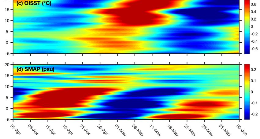
Remote Sens. 2020, 12, 3011                                                                        6 of 22

By comparing the difference in ocean color one week after and one week before the passage of Amphan,
however, we can see large blooms in the central Bay that follow the storm track, particularly in the
central Bay, where the productivity is comparable to that of coastal regions. There is an additional
bloom seen around 5◦ N and 85◦ E possibly related to the passage of the MJO or upwelling associated
with the smaller systems that later developed into Amphan. The gap-filled ocean color data nicely
demonstrate the extent to which Amphan impacted different regions of the Bay of Bengal. In the
following sections, we explore how the storm developed and influenced surface and mixed layer
processes in the Bay.

3.1.2. Multiparameter Analysis
      A multiparameter analysis of Cyclone Amphan before (Figure 2), during (Figure 3), and after
(Figure 4) the passage of the storm through the Bay of Bengal showed the response of the Bay to
the storm. Prior to cyclogenesis (Figure 2), there was scattered precipitation in the equatorial region
near Sri Lanka and in the Andaman Sea. In SLA, two large anticyclonic eddies could be observed
in the EICC region of the Bay, although most of the Bay is dominated by low SLAs and cyclonic
eddies (Figure 2B). SSTs at this time were in excess of 32 ◦ C (Figure 2C), with corresponding OHC
values near 8 × 10⁹ J/m2 in the north/central Bay, particularly west of 90◦ E (Figure 2E). SSS showed
reasonably low values in the majority of the Bay, with higher salinity along the east coast of India and
below 5◦ N. Surface winds were also reasonably calm in most of the Bay, with only near-equatorial
processes producing winds in excess of 10 m/s (Figure 2I). In the southern Bay, however, winds were
stronger than in other regions of the Bay, exceeding 5 m/s and being predominantly northeasterly
and easterly, with winds beginning to converge around the genesis region. Near-equatorial winds
across the northern Indian Ocean remained strong and were predominantly northwesterly over the
Arabian Sea. Surface fluxes (Figure 2J–L) showed that the majority out outward fluxes were confined
to the southern/central Bay (10◦ N, 82–95◦ E), with downward fluxes dominating the rest of the Bay. It is
notable that this is the region of cyclogenesis and is also where the highest magnitude surface winds
were observed in the Bay.
      The most striking feature of the pre-cyclone Bay, however, was the clear arrival of a downwelling
Kelvin wave, specifically the first downwelling Kelvin wave [46] at the Sumatra coast, which was
evident in SLA, BLT MLD, and ILD data (Figure 2B,F–H). This downwelling Kelvin wave drastically
increased MLD and ILD to below a 40 m depth in the equatorial region and increased BLT up to 10◦ N
in areas of the Bay.
      On 19 May, at the peak of storm intensity, precipitation was heavily concentrated at the center of
the storm in the northwestern Bay and skirting the edge of the coast (Figure 3A). Further precipitation
could be observed from 5–10◦ S near the Sumatra coast. The anticyclonic eddies in Figure 2B can be seen
to have decreased in radius (Figure 3B), particularly the northernmost eddy that was directly beneath
the storm. A clear upwelling pattern could be seen in the SST, SSS, and OHC data, with SSTs below 27
◦ C, an SSS exceeding 34 psu, and an OHC below 7 × 10⁹ J/m2 along the storm track (Figure 3C–E).

Directly below the storm, however, SSTs remained above 31 ◦ C and the OHC remained fairly high along
the coast, which continued to sustain the storm. Cyclone-strength winds were confined to the storm
center, although extremely high winds could be seen near the equator (0–5◦ N; Figure 3I). Moisture
and latent heat fluxes appeared to follow a similar pattern to surface wind (Figure 3I,J,L), with high
amplitude fluxes in regions of high surface wind. While sensible heat fluxes followed a similar pattern
(Figure 3K), there were pronounced positive fluxes in the western Bay, with negative fluxes in the
eastern Bay and in areas of high surface wind. The arrival of the first downwelling Kelvin wave was
pronounced (Figure 3B,F–H), with extremely high SLAs and BLT exceeding 40 m off the Sumatra coast.
In addition to the deepening of the mixed, barrier, and isothermal layers along the equator, there was
significant deepening observed along the storm track, with the ILD in the majority of the Bay exceeding
40 m.
Remote Sens.Remote
             2020,Sens.
                   12, 2020,
                        x FOR12, PEER
                                 3011 REVIEW                                                                                7 of 22        7 of 22

                  Figure 2. Multiparameter analysis of the Bay of Bengal on May 12, 2020 prior to cyclogenesis in
      Figure 2.(A)
                Multiparameter
                   Global Precipitation    analysis    of the
                                             Measurement        Bayprecipitation
                                                             (GPM)     of Bengal rateon (mm/day);
                                                                                          May 12, (B)2020   prior toMarine
                                                                                                         Copernicus    cyclogenesis
                                                                                                                            and       in (a)
               Environment      Monitoring     Service (CMEMS)     sea  level anomalies  (SLAs)  (cm)
      Global Precipitation Measurement (GPM) precipitation rate (mm/day); (b) Copernicus Marine and   overlaid with geostrophic
               currents (cm/s); (C) Nucleus for the European Modeling of the Ocean (NEMO) sea surface temperature
      Environment      Monitoring Service (CMEMS) sea level anomalies (SLAs) (cm) overlaid with
               (SST) data (◦ C); (D) NEMO sea surface salinity (SSS) data (psu); (E) 0–30 m ocean heat content (OHC;
      geostrophic
               J/m2currents       (cm/s);
                    * 109 ) calculated   from(c)NEMO;
                                                 Nucleus      for the
                                                        (F) barrier     European
                                                                    layer             Modeling
                                                                          thickness (BLT;           of the
                                                                                           m) calculated    Ocean
                                                                                                         from NEMO;(NEMO)
                                                                                                                      (G) mixed sea surface
               layer(SST)
      temperature     depth (MLD;
                              data (°C);m) calculated
                                               (d) NEMO from NEMO;       (H) isothermal
                                                               sea surface       salinitylayer  depth
                                                                                            (SSS)  data(ILD; m) calculated
                                                                                                          (psu);  (e) 0–30from
                                                                                                                             m ocean heat
               NEMO; (I) Cross-Calibrated        Multi-Platform    version  2 (CCMPv2)    surface wind  magnitude  (m/s; shaded)
      content (OHC; J/m2 * 109) calculated from NEMO; (f) barrier                          layer thickness (BLT; m) calculated from
               and vectors; (J) ERA5 instantaneous moisture flux (kg/m2 *day*10−3 ); (K) ERA5 surface sensible heat
      NEMO; (g)fluxmixed     layer
                    (J/m2 * 10         depth
                                6 ); and        (MLD;
                                          (L) ERA5        m)latent
                                                     surface   calculated
                                                                     heat fluxfrom
                                                                                (J/m2 NEMO;
                                                                                      * 107 ).   (h) isothermal layer depth (ILD; m)
      calculated from NEMO; (i) Cross-Calibrated Multi-Platform version 2 (CCMPv2) surface wind
      magnitude (m/s; shaded) and vectors; (j) ERA5 instantaneous moisture flux (kg/m2*day*10−3); (k)
      ERA5 surface sensible heat flux (J/m2 * 106); and (l) ERA5 surface latent heat flux (J/m2 * 107).

     On 19 May, at the peak of storm intensity, precipitation was heavily concentrated at the center
of the storm in the northwestern Bay and skirting the edge of the coast (Figure 3a). Further
precipitation could be observed from 5–10°S near the Sumatra coast. The anticyclonic eddies in Figure
2b can be seen to have decreased in radius (Figure 3b), particularly the northernmost eddy that was
directly beneath the storm. A clear upwelling pattern could be seen in the SST, SSS, and OHC data,
with SSTs below 27 °C, an SSS exceeding 34 psu, and an OHC below 7 × 10⁹ J/m2 along the storm track
(Figure 3c–e). Directly below the storm, however, SSTs remained above 31 °C and the OHC remained
Remote Sens. 2020, 12, x FOR PEER REVIEW                                                                                   8 of 22

exceeding 40 m off the Sumatra coast. In addition to the deepening of the mixed, barrier, and
isothermal layers along the equator, there was significant deepening observed along the storm track,
with  theSens.
   Remote ILD2020,
               in the   majority of the Bay exceeding 40 m.
                   12, 3011                                                                8 of 22

        Figure 3. Multiparameter analysis of the Bay of Bengal on May 19, 2020 at the peak of the storm in (A)
     Figure
        Global3. Precipitation
                 Multiparameter      analysis of(GPM)
                                 Measurement       the Bay   of Bengal on
                                                          precipitation      May
                                                                          rate     19, 2020(B)
                                                                               (mm/day);    at the peak of Marine
                                                                                               Copernicus   the storm
                                                                                                                    andin (a)
     Global   Precipitation
        Environment             Measurement
                         Monitoring              (GPM) sea
                                      Service (CMEMS)      precipitation   rate (SLAs)
                                                               level anomalies   (mm/day);    (b) Copernicus
                                                                                         (cm) overlaid          Marine and
                                                                                                        with geostrophic
     Environment
        currents (cm/s);Monitoring
                           (C) NucleusService      (CMEMS)
                                         for the European        sea level
                                                             Modeling   of the anomalies
                                                                               Ocean (NEMO) (SLAs)    (cm) temperature
                                                                                                sea surface  overlaid with
                      ◦
       (SST) data currents
                     ( C); (D) (cm/s);
                                NEMO (c)seaNucleus
                                             surface salinity
     geostrophic                                       for the(SSS)  data (psu);
                                                                European          (E) 0–30
                                                                            Modeling       m ocean
                                                                                        of the Ocean heat contentsea
                                                                                                       (NEMO)     (OHC;
                                                                                                                     surface
        J/m2 * 109 ) calculated
     temperature      (SST) datafrom  NEMO;
                                   (°C);       (F) barrier
                                          (d) NEMO      sealayer thickness
                                                             surface        (BLT;
                                                                       salinity   m) calculated
                                                                                (SSS)           from(e)
                                                                                       data (psu);    NEMO;
                                                                                                        0–30 m(G)ocean
                                                                                                                  mixedheat
        layer depth
     content   (OHC;(MLD;J/m2 *m)
                                109calculated
                                   ) calculatedfrom
                                                  fromNEMO;
                                                         NEMO;  (H)(f)
                                                                    isothermal   layerthickness
                                                                       barrier layer   depth (ILD;  m) m)
                                                                                                 (BLT;  calculated fromfrom
                                                                                                            calculated
        NEMO;    (I)  Cross-Calibrated  Multi-Platform    version  2 (CCMPv2)    surface  wind magnitude
     NEMO; (g) mixed layer depth (MLD; m) calculated from NEMO; (h) isothermal layer depth (ILD; m)        (m/s; shaded)
        and vectors; (J) ERA5 instantaneous moisture flux (kg/m2 *day*10−3 ); (K) ERA5 surface sensible heat
     calculated 2from6 NEMO; (i) Cross-Calibrated Multi-Platform                    version 2 (CCMPv2) surface wind
        flux (J/m * 10 ); and (L) ERA5 surface latent heat flux (J/m2 * 107 ).
     magnitude (m/s; shaded) and vectors; (j) ERA5 instantaneous moisture flux (kg/m2*day*10−3); (k)
     ERA5   surface
        Three   days sensible
                        after theheat  flux (J/m
                                  passage    of the* storm
                                                  2 106); and (l) ERA5 surface latent heat flux (J/m2 * 107).
                                                             in the Bay of Bengal, there was no notable precipitation
   or change in surface fluxes, although surface winds remained higher than prior to the cyclone and
     Three
   were      days after the
         predominantly       passage of the stormmore
                         southerly/southwesterly,  in theclosely
                                                           Bay offollowing
                                                                   Bengal, there   was monsoon
                                                                             southwest  no notable   precipitation
                                                                                                  climatology
or and
   change   in surface  fluxes, although   surface  winds   remained     higher   than prior to
        the conditions for monsoon onset (Figure 4A,I–L). The cold wake of the storm was apparentthe  cyclonein and
were
   SST, predominantly
        SSS, OHC, and ocean southerly/southwesterly,
                               color data, with upwelling more    closely
                                                            occurring  alongfollowing     southwest
                                                                               the storm track (Figures monsoon
                                                                                                         1 and
climatology
   4C–E). Theand   the conditions
               upwelling   signature for
                                      wasmonsoon   onset
                                          also apparent in (Figure   4a,i–l).
                                                            mixed layer       The coldparticularly
                                                                          parameters,   wake of the MLDstorm
                                                                                                           andwas
apparent in SST, SSS, OHC, and ocean color data, with upwelling occurring along the storm track
Remote Sens. 2020, 12, x FOR PEER REVIEW                                                                                        9 of 22

  Remote Sens. 2020, 12, 3011                                                                                              9 of 22
(Figures 1 and 4c–e). The upwelling signature was also apparent in mixed layer parameters,
particularly MLD and ILD, where there was a shoaling of the mixed layer and isothermal layer
  ILD, where
directly to thethere
                westwas   a shoaling
                      of the         of theand
                             storm track     mixed   layer and of
                                                a deepening      isothermal  layer
                                                                    both to the    directly
                                                                                east of theto the west
                                                                                            storm      of the
                                                                                                   (Figure  4f–h).
  storm  track and a deepening  of both  to the east  of the storm  (Figure 4F–H). SLAs   did
SLAs did not appreciably change, though the progression of the downwelling coastal Kelvin wavenot appreciably
  change,
along  the though
           edge ofthe
                   theprogression
                        eastern Bayofwas
                                      the downwelling
                                           apparent (Figurecoastal Kelvin wave along the edge of the eastern
                                                                 4c).
  Bay was apparent (Figure 4C).

        Figure 4. Multiparameter analysis of the Bay of Bengal on May 23, 2020 after the storm in (A) Global
     Figure   4. Multiparameter
       Precipitation   Measurementanalysis     of the Bay of
                                      (GPM) precipitation    rateBengal   on May
                                                                  (mm/day);         23, 2020 after
                                                                              (B) Copernicus        theand
                                                                                               Marine    storm    in (a) Global
                                                                                                             Environment
     Precipitation     Measurement
       Monitoring Service    (CMEMS) sea (GPM)      precipitation
                                             level anomalies   (SLAs)rate
                                                                        (cm)(mm/day);
                                                                             overlaid with(b)   Copernicus
                                                                                            geostrophic           Marine
                                                                                                           currents  (cm/s); and
     Environment
       (C) Nucleus for Monitoring
                          the European Service    (CMEMS)
                                           Modeling              sea level
                                                       of the Ocean     (NEMO) anomalies    (SLAs)
                                                                                   sea surface         (cm) overlaid
                                                                                               temperature     (SST) datawith
       (◦ C); (D) NEMO
     geostrophic          sea (cm/s);
                    currents   surface (c)
                                        salinity (SSS)for
                                           Nucleus     data
                                                          the(psu);  (E) 0–30
                                                               European        m ocean of
                                                                            Modeling     heat
                                                                                           thecontent
                                                                                               Ocean(OHC;
                                                                                                        (NEMO)      2 * 109 )
                                                                                                                J/msea   surface
       calculated from
     temperature     (SST)NEMO;    (F) barrier
                            data (°C);          layer thickness
                                         (d) NEMO      sea surface(BLT;   m) calculated
                                                                       salinity          from(psu);
                                                                                 (SSS) data    NEMO; (e) (G)
                                                                                                          0–30mixed    layer heat
                                                                                                                 m ocean
       depth (OHC;
     content   (MLD; m)J/mcalculated   from NEMO;
                           2 * 109) calculated   from(H)   isothermal
                                                        NEMO;            layer depth
                                                                   (f) barrier        (ILD; m) calculated
                                                                                layer thickness  (BLT; m)from      NEMO;from
                                                                                                              calculated
       (I) Cross-Calibrated Multi-Platform version 2 (CCMPv2) surface wind magnitude (m/s; shaded) and
     NEMO; (g) mixed layer depth (MLD; m) calculated from NEMO; (h) isothermal layer depth (ILD; m)
       vectors; (J) ERA5 instantaneous moisture flux (kg/m2 *day*10−3 ); (K) ERA5 surface sensible heat flux
     calculated   from NEMO; (i) Cross-Calibrated Multi-Platform version 2 (CCMPv2) surface wind
       (J/m2 * 106 ); and (L) ERA5 surface latent heat flux (J/m2 * 107 ).
     magnitude (m/s; shaded) and vectors; (j) ERA5 instantaneous moisture flux (kg/m2*day*10−3); (k)
     ERA5 surface sensible heat flux (J/m2 * 106); and (l) ERA5 surface latent heat flux (J/m2 * 107).

3.2. Impacts on the Bay of Bengal
    To investigate the impact of Amphan on the Bay of Bengal, a box-averaged cross-section of the
Bay was taken along the storm track at 14°N, where the minimum central pressure (907 mb) was felt
Remote Sens. 2020, 12, 3011                                                                                                   10 of 22

3.2. Impacts on the Bay of Bengal
Remote Sens. 2020, 12, x FOR PEER REVIEW                                                                                      10 of 22
      To investigate the impact of Amphan on the Bay of Bengal, a box-averaged cross-section of the Bay
at the
was     peakalong
     taken    of storm    intensity
                     the storm   track  at 14◦5).
                                     (Figure   N, Prior
                                                   wheretothe theminimum
                                                                   arrival of central
                                                                              the storm,   salinity
                                                                                      pressure       was
                                                                                                   (907 mb)low  in the
                                                                                                              was   felt upper
                                                                                                                         at the
60  m  of  the  water   column,     with  values  of
Remote Sens. 2020, 12, 3011 11 of 22
Remote Sens. 2020, 12, x FOR PEER REVIEW 11 of 22
Figure 6. Box-averaged time series from May 9 to May 27, 2020 in the northern (86–88◦ E, 15–20◦ N;
Figure 6. Box-averaged time series from May 9 to May 27, 2020 in the northern (86–88°E, 15–20°N;
black), central (86–88 ◦ E, 10–15◦ N; blue), and southern (86–88◦ E, 5–10◦ N; red) Bay of Bengal for (A) GPM
black), central (86–88°E, 10–15°N; blue), and southern (86–88°E, 5–10°N; red) Bay of Bengal for (a)
precipitation (mm/day);
GPM precipitation (B) CCMPv2
(mm/day); surfacesurface
(b) CCMPv2 wind magnitude (m/s);(m/s);
wind magnitude (C) CMEMS geostrophic
(c) CMEMS surface
geostrophic
currents (cm/s); (D) CMEMS SLA (cm); (E) OISST (◦ C); and (F) SMAP SSS (psu).
surface currents (cm/s); (d) CMEMS SLA (cm); (e) OISST (°C); and (f) SMAP SSS (psu).
While satellite
While observations
satellite observationslargely
largely followed patternsofof
followed patterns cyclone
cyclone intensity,
intensity, withwith the central
the central Bay Bay
experiencing the most pronounced response to the passage of Amphan, mixed
experiencing the most pronounced response to the passage of Amphan, mixed layer parameters layer parameters
(Figure
(Figure 7A–D)7a–d)
and and surfacefluxes
surface fluxes(Figure
(Figure 7E–G)
7e–g) more
moreclosely
closelyaligned
alignedwith precipitation
with (Figure
precipitation 6a). 6A).
(Figure
BLT was deepest in the central Bay following the maximum changes in salinity
BLT was deepest in the central Bay following the maximum changes in salinity and temperature and temperature
(Figure 7a); however MLD and ILD were both strongest in the southern Bay with a gradient of depths
(Figure 7A); however MLD and ILD were both strongest in the southern Bay with a gradient of depths
by latitude (Figure 7b–c). This followed the spatial patterns seen in Figures 2–4, where MLD and ILD
by latitude (Figure 7B,C). This followed the spatial patterns seen in Figures 2–4, where MLD and
both deepened most clearly in response to the downwelling Kelvin wave in the near-equatorial
ILD both deepened
region. A 0–30 mmostOHC clearly
followed inpatterns
response of to the downwelling
cyclone intensity, withKelvin wave
the central instarting
Bay the near-equatorial
off with
region. A 0–30 m OHC followed patterns of cyclone intensity, with the central Bay starting off with at
least 1 × 10⁸ J/m2 more heat than the other regions. While small compared to overall OHC values,
small changes in the OHC could still contribute to SSTs, latent heat fluxes, and available atmospheric
moisture. The warm central Bay can most clearly be seen in Figure 2E, which shows that there wereRemote Sens. 2020, 12, x FOR PEER REVIEW 12 of 22
at least 1 × 10⁸ J/m2 more heat than the other regions. While small compared to overall OHC values,
smallRemote
changes in the
Sens. 2020, OHC could still contribute to SSTs, latent heat fluxes, and available atmospheric
12, 3011 12 of 22
moisture. The warm central Bay can most clearly be seen in Figure 2e, which shows that there were
clearly much higher OHC values in the central Bay and along the storm track, likely contributing to
clearly much higher OHC values in the central Bay and along the storm track, likely contributing to
the resulting cyclone intensity.
the resulting cyclone intensity.
Figure 7. Box-averaged time series from May 9 to May 27, 2020 in the northern (86–88◦ E,
Figure 7. Box-averaged time series from May 9 to May 27, 2020 in the northern (86–88°E, 15–20°N;
15–20◦ N; black), central (86–88◦ E, 10–15◦ N; blue), and southern (86–88◦ E, 5–10◦ N; red) Bay of
black), central (86–88°E, 10–15°N; BLT
Bengal for: (A) NEMO-derived blue),
(m);and
(B) southern (86–88°E,
NEMO-derived MLD5–10°N; red) Bay of Bengal
(m); (C) NEMO-derived ILD (m);for: (a)
NEMO-derived BLT (m);
(D) NEMO-derived 0–30(b) NEMO-derived
m OHC MLD
(J/m2 * 109 ); (E) ERA5(m); (c) NEMO-derived
instantaneous moisture fluxILD (m);
(kg/m (d) NEMO-
2 *day*10 −3 );
derived 0–30 m OHC (J/m 2 * 109); (e) ERA5
2 instantaneous
6 moisture flux (kg/m 2*day*102 −3); 7(f) ERA5
(F) ERA5 surface sensible heat flux (J/m * 10 ); and (G) ERA5 surface latent heat flux (J/m * 10 ).
surface sensible heat flux (J/m2 * 106); and (g) ERA5 surface latent heat flux (J/m2 * 107).
Surface fluxes more closely followed patterns of precipitation, with the highest magnitude fluxes
in the
Surfacenorthern Bay onclosely
fluxes more May 19followed
and lowerpatterns
values seen in the central with
of precipitation, and southern Bay magnitude
the highest (Figure 7E–G). fluxes
Latent heat fluxes are widely considered to be the primary fuel for cyclone intensity, and so while
in the northern Bay on May 19 and lower values seen in the central and southern Bay (Figure 7e–g).
they were not the most important factor for observed minimum pressure and wind speed magnitude,
Latent heat fluxes are widely considered to be the primary fuel for cyclone intensity, and so while
these surface fluxes did help to increase the volume of precipitation associated with the storm in the
they were not the most important factor for observed minimum pressure and wind speed magnitude,
northern Bay.
these surface fluxes did help to increase the volume of precipitation associated with the storm in the
northern Bay.Remote
Remote Sens.
Sens. 12,x 3011
2020,12,
2020, FOR PEER REVIEW 1313ofof2222
3.3. Equatorial Processes
3.3. Equatorial Processes
In order to better assess the propagation of the storm system, an unfiltered time–latitude plot
In order to better assess the propagation of the storm system, an unfiltered time–latitude plot for
for the storm track in the Bay of Bengal and equatorial region (86–88°E, −5–20°N) was created (Figure
the storm track in the Bay of Bengal and equatorial region (86–88◦ E, −5–20◦ N) was created (Figure 8).
8). The genesis, strengthening, and northward propagation of Amphan from May 14 to May 20 can
The genesis, strengthening, and northward propagation of Amphan from May 14 to May 20 can
be clearly seen in Figure 8a, with smaller systems dominating the southern Bay and equatorial region
be clearly seen in Figure 8a, with smaller systems dominating the southern Bay and equatorial
beginning in Aprilinthat
region beginning Aprilincreased in both
that increased frequency
in both frequencyandandintensity ininthe
intensity theweeks
weeks leading uptoto
leading up
cyclogenesis.
cyclogenesis.Satellite
Satelliteobservations
observationsofofSLAs,
SLAs,SST,
SST, and
and SSS
SSS all reflected the
all reflected the upwelling
upwellingandandcold
coldwake
wake
along the storm track following the passage of the storm, with a particularly stark contrast
along the storm track following the passage of the storm, with a particularly stark contrast in SST and in SST and
SSS
SSSbeing
beingapparent.
apparent. While
While SSS reboundedtotopre-cyclone
SSS rebounded pre-cyclone values
values fairly
fairly quickly,
quickly, bothboth
SLAsSLAs anddid
and SST SST
did not return to pre-cyclone values even by the end of May and the beginning
not return to pre-cyclone values even by the end of May and the beginning of the southwest monsoonof the southwest
monsoon season. Regarding
season. Regarding SLAs, of
SLAs, the arrival thethearrival of the firstKelvin
first downwelling downwelling
wave wasKelvin wave was
most apparent most
around
apparent around
the equator, themaximum
with the equator, inwith
SLAsthe maximum
occurring in SLAs
concurrently withoccurring concurrently
both cyclogenesis withstorm
and peak both
cyclogenesis and peak
intensity (Figure 8b). storm intensity (Figure 8b).
Figure 8. Time–latitude plots of (a) GPM precipitation rate (mm/day), (b) CMEMS SLA (cm), (c) OISST
Figure 8. Time–latitude plots of (a) GPM precipitation rate (mm/day), (b) CMEMS SLA (cm), (c) OISST
(◦ C), and (d) SMAP SSS (psu) in the Bay of Bengal (86–88◦ E, −5–20◦ N) from April 1 to May 31, 2020
(°C), and (d) SMAP SSS (psu) in the Bay of Bengal (86–88°E, −5–20°N) from April 1 to May 31, 2020
with the seasonal cycle removed.
with the seasonal cycle removed.Remote Sens. 2020, 12, 3011 14 of 22
Remote Sens. 2020, 12, x FOR PEER REVIEW 14 of 22
Given
Giventhe therelative
relativedominance
dominance of of equatorial processesininSLAs
equatorial processes SLAsand andthethetiming
timingof of
thethe first
first
downwelling Kelvin wave, the time–latitude
downwelling Kelvin wave, the time–latitude fields in Figure 8 were next 30–90-day bandpass
in Figure 8 were next 30–90-day bandpass filtered filtered
with
withthethe
seasonal
seasonal cycle
cycleremoved
removedfor forthe
thetimescale
timescaleofofthe
theMJO,
MJO,the thepassage
passageof ofwhich
whichhashas been
been noted
noted by
several previous
by several studies
previous [5,17–19]
studies to trigger
[5,17–19] cyclogenesis
to trigger in thisinregion
cyclogenesis (Figure
this region 9). The
(Figure 9).bandpass filtered
The bandpass
filtered
fields fields
indeed indeed ashowed
showed a pronounced
pronounced 30–90-day30–90-day
mode in mode in allsatellite
all four four satellite parameters,
parameters, withwith a
a strong
strong 30–90-day
30–90-day signal occurring
signal occurring at the sameat the
timesame time as cyclogenesis
as cyclogenesis in the Bay.inThis
the was
Bay. most
This pronounced
was most
in pronounced
SLAs and SST in SLAs and9b,c),
(Figure SST (Figure
with the9b,c), with the maximum
maximum in SST occurring
in SST occurring in the region
in the genesis genesisjust
region
prior
just prior
to cyclogenesis.to cyclogenesis.
Figure 9.9.30–90-day
Figure 30–90-day bandpass filteredtime–latitude
bandpass filtered time–latitude plots
plots of GPM
of (a) (a) GPM precipitation
precipitation rate (mm/day),
rate (mm/day), (b)
(b)CMEMS
CMEMSSLA SLA(cm),
(cm),(c)(c)OISST ◦
OISST(°C),
( C),and
and(d)(d) SMAP SSS (psu) (86–88◦ E, −5–20◦ N)
SMAP SSS (psu) inin the
the Bay
Bay ofof Bengal
Bengal (86–88°E, −5–20°N)
from April
from April1 to
1 toMay
May31,31,2020
2020with
withthe
theseasonal
seasonal cycle removed.
cycle removed.
3.4. Impact on Southwest Monsoon Onset
3.4. Impact on Southwest Monsoon Onset
Given the timing of Amphan and the passage of the MJO through the equatorial Indian Ocean in
Given the timing of Amphan and the passage of the MJO through the equatorial Indian Ocean
late May, we next
in late May, weturned our attention
next turned to the southeastern
our attention Arabian
to the southeastern Sea where
Arabian Sea the southwest
where monsoon
the southwest
began on June 1, 2020, in accordance with climatology. The anomalously strong positive IOD
monsoon began on June 1, 2020, in accordance with climatology. The anomalously strong positive in 2019
modified coastal Kelvin wave propagation in the Bay and reduced the strength of the EICC flow intoRemote Sens. 2020, 12, x FOR PEER REVIEW 15 of 22
Remote Sens. 2020, 12, 3011 15 of 22
IOD in 2019 modified coastal Kelvin wave propagation in the Bay and reduced the strength of the
EICC
the flow into the southeastern
southeastern Arabian Sea. Arabian
PreviousSea. Previous
studies studies
[26,49,50] [26,49,50]
have shown have shown thatfluxes
that freshwater freshwater
into this
fluxes
regioninto
arethis region
critical for are criticalonset
monsoon for monsoon onsetfollowing
and that onset and thata onset following
positive a positive
IOD is typically IOD is
delayed due
typically delayed due to the associated dynamics. Despite these apparent setbacks,
to the associated dynamics. Despite these apparent setbacks, the 2020 southwest monsoon onset with the 2020
southwest monsoon
climatology onset
on June withunfiltered
1. An climatology on June 1. An
time–latitude plotunfiltered time–latitude
of this region (65–60◦ E,plot of this
−5–20 ◦ N) region
revealed
(65–60°E, −5–20°N)
a northward revealed of
propagation a northward
precipitationpropagation
beginningof precipitation
after beginning
May 1 (Figure after May
10a). While 1 (Figure
the propagation
10a).
wasWhile theapparent
not as propagation was not
in SLAs, as apparent
a northward in SLAs, a of
propagation northward
high SSTspropagation
in excess ofof31high SSTs inare
◦ C, which
excess of 31 °C,
associated which
with are associated
the Arabian Sea Miniwith
Warmthe Arabian Sea Mini
Pool [25,26,30], Warm
began in Pool
April[25,26,30], began
and preceded in April
precipitation
and preceded precipitation by two weeks (Figure 10c). No
by two weeks (Figure 10c). No clear propagation was apparent in SSS.clear propagation was apparent in SSS.
Figure
Figure 10.10. Time–latitude
Time–latitude plotsofof(a)
plots (a)GPM
GPM precipitation
precipitation rate
rate(mm/day),
(mm/day),(b)(b)
CMEMS SLA
CMEMS (cm),
SLA (c) OISST
(cm), (c)
( ◦ C), and (d) SMAP SSS (psu) in the southeastern Arabian Sea (65–70◦ E, −5–20◦ N) from April 1 to
OISST (°C), and (d) SMAP SSS (psu) in the southeastern Arabian Sea (65–70°E, −5–20°N) from April
1 toMayMay31,31,2020
2020with
withthe
theseasonal
seasonalcycle
cycleremoved.
removed.
To identify the impact of potential MJO propagation on southwest monsoon onset, the time–latitude
To identify the impact of potential MJO propagation on southwest monsoon onset, the time–
fields in Figure 10 were bandpass-filtered for the 30–90-day range (Figure 11) as in Figure 9.
latitude fields in Figure 10 were bandpass-filtered for the 30–90-day range (Figure 11) as in Figure 9.
The northward propagation of the MJO system (BSISO) in precipitation is apparent in Figure 11a,
The northward propagation of the MJO system (BSISO) in precipitation is apparent in Figure 11a,
with precipitation increasing on May 1 and extending northward through monsoon onset. The equatorial
with precipitation increasing on May 1 and extending northward through monsoon onset. TheRemote Sens. 2020, 12, 3011 16 of 22
Remote Sens. 2020, 12, x FOR PEER REVIEW 16 of 22
equatorial propagation
propagation of MJO
of the oceanic the oceanic MJOin
is apparent is all
apparent in all three with
three parameters, parameters, withofthe
the timing timing SSTs
warming of
warming
(Figure 11c)SSTs
and(Figure 11c) andwave
the planetary the planetary wave(Figure
propagation propagation (Figure 11b)
11b) preceding preceding precipitation.
precipitation.
Figure 11.30–90-day
Figure11. 30–90-dayfiltered
filteredtime–latitude plots of
time–latitude plots of (a)
(a)GPM
GPMprecipitation
precipitationrate
rate(mm/day),
(mm/day),(b)(b) CMEMS
CMEMS
SLA (cm), (c) OISST ( ◦ C), and (d) SMAP SSS (psu) in the southeastern Arabian Sea (65–70◦ E, −5–20◦ N)
SLA (cm), (c) OISST (°C), and (d) SMAP SSS (psu) in the southeastern Arabian Sea (65–70°E, −5–20°N)
from
fromApril
April1 1totoMay
May31,31,2020
2020with
withthe
the seasonal
seasonal cycle removed.
cycle removed.
The passage of the MJO through the equatorial Indian Ocean was accompanied by the triggering
The passage of the MJO through the equatorial Indian Ocean was accompanied by the triggering
ofof
a northward-propagating
a northward-propagatingBSISO BSISOevent
event (Figures 11 and
(Figures 11 and 12).
12).AsAsthis
thisBSISO
BSISOevent
eventmoved
moved northward
northward
through
throughthetheArabian
ArabianSea, Sea, the
the MJO
MJO continued
continued toto propagate
propagate eastward,
eastward,withwiththethefurther
furthernorthward
northward
propagation of planetary wave activity triggering cyclogenesis in the Bay of Bengal
propagation of planetary wave activity triggering cyclogenesis in the Bay of Bengal and ultimately and ultimately
leading
leadingtotothe
theformation
formationof ofCyclone
Cyclone Amphan.
Amphan. The The passage
passageofofthetheBSISO
BSISOandandthetheeffects
effectsofofAmphan
Amphan
were strongly felt in the southeastern Arabian Sea in moisture flux, with a minimum
were strongly felt in the southeastern Arabian Sea in moisture flux, with a minimum on May 17–18 on May 17–18
that reached nearly −0.12 kg/m 22s. Moisture flux values associated with these systems in mid-May
that reached nearly −0.12 kg/m Moisture flux values associated with these systems in mid-May
exceeded
exceededthe themonsoon
monsoon onset responseon
onset response onJune
June1–2,
1–2,which
which was
was atypical
atypical of the
of the usualusual gradual
gradual buildbuild
of
ofmoisture
moistureobserved
observed inin other
other years.
years. Though
Though the the passage
passage of tropical
of tropical systems
systems throughthrough this region
this region is not is
not uncommon
uncommon prior
prior to to monsoon
monsoon onset,
onset, thethe unique
unique combination
combination of of BSISO
BSISO passage,
passage, tropical
tropical cyclone
cyclone
formation, and timing helped to precondition the southeastern Arabian Sea to a state that likelyRemote Sens. 2020, 12, x FOR PEER REVIEW 17 of 22
formation, and
Remote Sens. timing helped to precondition the southeastern Arabian Sea to a state
2020, 12, 3011 that likely
17 of 22
contributed to the timing, location, and strength of the onset given the available atmospheric
moisture at the time.
contributed to the timing, location, and strength of the onset given the available atmospheric moisture
at the time.
Figure 12. Spatial plots of GPM precipitation rate (shaded; mm/day) for: (A) May 14, (B) May
Figure 12.
15, Spatial
(C) May plots of May
16, (D) GPM 17,precipitation
(E) May 18, (F) rate (shaded;
May 19, (G) mm/day)
May 31, (H)for: (a)1,May
June and 14, (b) May
(I) June 2, 15, (c)
with (J) a box-averaged time series of ERA5 instantaneous moisture flux data (kg/m 2 *s*10−3 ) in the
May 16, (d) May 17, (e) May 18, (f) May 19, (g) May 31, (h) June 1, and (i) June 2, with (j) a box-
southeastern Arabian Sea (65–70◦ E, 6–13◦ N) from May 1 to June 5, 2020.
averaged time series of ERA5 instantaneous moisture flux data (kg/m *s*10 ) in the southeastern
2 −3
Arabian Sea (65–70°E, 6–13°N) from May 1 to June 5, 2020.
4. Discussion
4.1. Cyclogenesis
The multiparameter analysis of Cyclone Amphan revealed that the genesis of storm occurredRemote Sens. 2020, 12, 3011 18 of 22
4. Discussion
4.1. Cyclogenesis
The multiparameter analysis of Cyclone Amphan revealed that the genesis of storm occurred
concurrently with the passage of an oceanic downwelling Kelvin wave (Figures 2–4) and the MJO
(Figures 8 and 9). Previous studies of tropical cyclone activity have analyzed the impact of tropical waves
on cyclogenesis [4,5,14,17,18,51], both globally and in the northern Indian Ocean. While there have been
several studies that have analyzed the impact of atmospheric Kelvin waves on cyclogenesis [5,14,17,19],
finding them to have the greatest impact on cyclogenesis in Northern Hemisphere in spring [5], fewer
have focused on the impact oceanic planetary waves have on cyclogenesis [4]. A 2010 case study of
Cyclone Nargis (2008) in the Bay of Bengal [4] found that the passage of a downwelling off-equatorial
Rossby Wave in the Bay ultimately caused a shoaling of the mixed layer and raised SSTs, helping
to alter the cyclone track. While Rossby waves were not apparently involved in directing the track
of Cyclone Amphan, our analysis suggested that the arrival of an equatorial downwelling Kelvin
wave and the successive propagation of a downwelling coastal Kelvin wave helped to depress the
thermocline and increase local SSTs, 0–30 m OHC, MLD, ILD, and BLT (Figures 2–4). While this
occurred closer to the equator, a multiparameter analysis of the conditions before and during the storm
suggested that the passage of the oceanic Kelvin wave did help to precondition the genesis region for
cyclone development (Figures 3 and 4).
Despite the timing of this Kelvin wave and its significant impact on the upper ocean, another
equatorial wave-like phenomenon was more dominantly involved in Amphan’s development: the MJO.
Previous studies have repeatedly shown that the MJO is a key contributor to global cyclogenesis [5,17,19].
One such study found that the spring peak in northern Indian Ocean cyclogenesis occurred concurrently
with statistical peaks in MJO, equatorial Rossby wave, and Kelvin wave activity [5]. This study found
that waves enhanced low level vorticity and that the storms that formed along the convectively active
portion of the wave helped to enhance deep convection in the genesis region that ultimately led to
genesis. This was consistent with our findings, where the passage of the positive (convective) phase of
the MJO initiated several smaller storms in the near-equatorial Bay that later developed and organized
into Amphan (Figures 2, 9 and 12).
While equatorial waves undoubtedly played a significant role in cyclogenesis, it was also the
northward-propagating BSISO, related to the MJO, and its associated convection that likely helped to
trigger cyclogenesis (Figure 12). Previous studies of cyclogenesis in the Bay have found that the most
favorable conditions for cyclogenesis occur in May and October–November, due to a weak vertical
shear, as well as that the passage of the BSISO also produces high absolute vorticity and relative
humidity [18]. This was likely the case with Cyclone Amphan, which was generated in May following
the passage of the MJO and BSISO.
4.2. Southwest Monsoon Onset
The 2020 southwest monsoon onset occurred on June 1, 2020 over the southwestern state of
Kerala. The timing of Amphan and the MJO were both such that the moisture flux and precipitation
associated with both systems helped to precondition the southeastern Arabian Sea for monsoon onset
and helped to ensure that onset occurred on time. Studies of the conditions necessary for southwest
monsoon onset have found that there is a convergence of heat and moisture in the eastern Bay of
Bengal [20], such as that observed concurrently with Cyclone Amphan (Figures 2–4 and 12). Onset is
then characterized by a convergence of heat, moisture, and diabatic heating over the Arabian Sea,
with increased low-level kinetic energy and net tropospheric moisture over the same region [20].
The moisture flux and increasing SSTs in the southeastern Arabian Sea impacted by both Amphan and
the MJO helped to create these necessary conditions in the Arabian Sea for monsoon onset to occur
(Figures 10–12).Remote Sens. 2020, 12, 3011 19 of 22
The MJO and the northward-propagating BSISO have been shown by previous studies, and they
are well-known to impact monsoon onset and variability [20–24,51,52]. It has been found that the
phase of the MJO and the location of its convective center can heavily impact the timing and strength of
monsoon onset [21], and a normal onset occurs when the MJO is in the western Indian Ocean. Beyond
the contributions of moisture and convection to the southeastern Arabian Sea, the MJO and BSISO help
to establish low-level westerlies in this region and also impact nonlinear eddy momentum transport,
which helps to create the conditions necessary for onset to occur [23,24]. It would seem that this was
the case in 2020, where the passage of the MJO, BSISO, and Amphan transported moisture into the
southeastern Arabian Sea and established surface northwesterly winds over the southeastern Arabian
Sea. Thus, is appears that this perfect storm of tropical systems all worked together to allow for 2020 to
have a climatological onset despite occurring after a strong positive IOD year [6].
With the changing climate and the relative importance of ISOs and synoptic systems in determining
monsoon onset, it is now, more than ever, crucial that we improve our monitoring and forecasting of
these systems through improved observations and modeling. Because the MJO and BSISO, as well
as tropical cyclones and monsoon onset, are all highly coupled systems, it is increasingly clear that
the accurate forecasting and modeling of these events will rely on high quality remotely sensed
observations and the assimilation of these data into modeled forecasts.
5. Conclusions
The MJO is the dominant form of intraseasonal variability in the tropics that impacts tropical
cyclogenesis and informs monsoon strength and onset. This has thus far been in the case leading into
the 2020 monsoon season, as the MJO and BSISO have been seen to impact the cyclogenesis of Cyclone
Amphan (2020), which developed into an intense tropical system, and southwest monsoon onset.
Cyclone Amphan (2020) developed into an exceptionally intense storm, reaching a minimum
central pressure of 907 mb on May 19 and unleashing almost 400 mm/day of precipitation in the
northern Bay of Bengal. This storm was allowed to rapidly intensify due to an exceptionally high 0–30 m
OHC and the arrival of a downwelling equatorial Kelvin wave, which depressed the thermocline,
increased SSTs, deepened the mixed layer, and helped to precondition the southern Bay of Bengal for
cyclogenesis. Cyclogenesis occurred around 8◦ N following the passage of the convective phase of
the MJO, which released a northward-propagating BSISO that helped to provide the moisture and
pre-existing convection necessary for cyclogenesis.
In addition to impacting Amphan’s cyclogenesis, the passage of the MJO also impacted southwest
monsoon onset. The northward-propagating BSISO and equatorial MJO both helped to set up the
low-level westerlies in the southeastern Arabian Sea, as well as to transport moisture into the onset
region. Further moisture was then transported in conjunction with Amphan, which actually produced
a greater moisture flux in the southeastern Arabian Sea than the onset itself. The timing and intensity of
these events all worked together to allow for monsoon onset to occur on June 1 despite the exceptionally
low freshwater flux into the southeastern Arabian Sea due to the strong positive IOD in 2019.
This complex interplay of mixed layer processes, ISOs, tropical cyclones, planetary waves,
and monsoon onset highlights our continuing need for high resolution, high quality, near real-time
observations from satellites to better inform model forecasts. ISO forecasting and cyclone intensity
forecasting both remain difficult, and improved observations and the assimilation of these observations
will help to improve these forecasts. The southwest monsoon and tropical cyclones in the Bay of Bengal
directly impact well over a billion people, and it is thus critical that, moving forward, we improve our
monitoring, understanding, and forecasting of these complex phenomena.
Author Contributions: H.L.R.-S. and B.S. conceived and designed the data analysis and interpretation of the
results. H.L.R.-S. prepared all the figures and writing of this article, and B.S. designed the project, guided this
work, and corrected the paper. All authors have read and agreed to the published version of the manuscript.You can also read


