Forecasting with Competing Models of Daily Bitcoin Price in R

Forecasting with Competing Models…. Adekunle, Gbadebo, Akande, & Adedokun

 Journal of Studies in Social Sciences and Humanities
 http://www.jssshonline.com/
 Volume 8, No. 2, 2022, 272-287
 ISSN: 2413-9270

 Forecasting with Competing Models of Daily Bitcoin Price in R
 Oluwatobi A. Adekunle
 E-mail: tobiahamed@yahoo.com
 Department of Accounting Science,
 Walter Sisulu University, Mthatha, Eastern Cape, South Africa

 Adedeji D. Gbadebo*
 E-mail: gbadebo.adedejidaniel@gmail.com
 Department of Accounting Science,
 Walter Sisulu University, Mthatha, Eastern Cape, South Africa

 Joseph O. Akande
 E-mail: jakande@wsu.ac.za
 Department of Accounting Science,
 Walter Sisulu University, Mthatha, Eastern Cape, South Africa

 Muri W. Adedokun
 E-mail: muri.adedokun@akun.edu.tr
 Department of Accounting and Finance,
 University of Mediterranean Karpasia, Nicosia, Turkey

Abstract
Bitcoin price exhibits patterns predictable on its historical pasts. We adopt ARIMA(auto), ARIMA(fix)
models and the Holt-Winters filter (HWF) with trend plus additive seasonal HWF ( [0,1]), and no
seasonality HWF ( [False]) to forecast the price of Bitcoin under three datasets–Actual (observed),
Polynomial (fitted) and STL-Trend (fitted). We apply daily time-series from 1/09/2014–28/12/2020,
and establish 18 models to forecast the price of Bitcoin. The results show that HWF ( [0,1]) with lower
limit fitted on STL-Trend provides the best prediction on the first training-sample, while ARIMA(fix)
fitted on actual data outperform in the second training-set with the smallest Mean-Absolute-Error
(MAE). The training-set forecast performance of the ARIMA(fix) for the actual function provides better
performance with the least MAE. The HWF is appropriate for prediction of the daily Bitcoin price with
the generalise STL-Trend function, but ARIMA(fix) is more accurate for the actual series.

Keywords: Bitcoin, ARIMA, Holt-Winters, Mean Absolute Error

 Introduction
The cryptocurrency ‘Bitcoin (BTC)’ has generated consistent attention in recent years. BTC has global
influences, leading to change in payment methods, financial assets and monetary policies (Pabuçcu,
Ongan & Ongan, 2020). The virtual currency shares attribute as fiat money and speculative assets (Baur,
Hong & Lee, 2018). There are concerns by investors, traders and researchers about the pattern of the
daily price movement. The highly volatile digital currency is associated with significant price swings
in hourly, daily and long-term valuations since its invention (Hung, Liu & Yang, 2020). Bitcoin price
rises by 1000% from $0.008 in 12 July to $0.08 in 17 July, 2010. It becomes parity with US dollars on
Feb 15, 2011 and reaches a landmark high of above $19,500 on 18 December, 2017. Since Mid-

 272 JSSSH – An international online research journal in social sciences and humanities

Forecasting with Competing Models…. Adekunle, Gbadebo, Akande, & Adedokun

December 2020, the price has experienced a meteoric rise fluctuation between $24,000 and $27,000
which is reported to be above 40% gains from its 2017 peak.
 The sporadic volatility of Bitcoin price has prompted attempts to forecast its daily future price
(Munim, Shakil & Alon, 2019; Chen, Li & Sun, 2020). The price of Bitcoin has exhibited patterns
which is largely predictable upon its historical past. Developing a suitable and accurate forecast model
for next-day forecast of its price may increase traders’ returns and trading activities (Munim et al.,
2019). In addition, the fact that Bitcoin is continuously traded even less stronger currencies makes
prediction of its price inevitable. The information asymmetric, dynamic behaviours of miners and
uncertainties in the cryptocurrency markets make forecasting the price of Bitcoin a challenging task
(Kliber et al., 2019). The choice of the forecasting model can have a significant effect on the
performance of Bitcoin and the make the cryptocurrency market more efficient (Caporale, Gil-Alana,
& Plastun, 2018). This paper aims to find a model that enables accurate forecast of daily Bitcoin price.
 We establish forecast interval that can guide market participants in the speculation of Bitcoin
price. We extend the frontier of research in two ways. First, available studies (McNally, Roche & Caton,
2018; Munim et al., 2019; Mudassir et al., 2020) forecast Bitcoin price with actual time-series. There
is need for generalise function data to be applied for empirical analysis, particularly for forecasting
rather than actual data with which we construct the general function. Hence, our study establishes
predictions predicated upon two generalisation of the daily Bitcoin price time-series. The investigations
allow us to partition the dataset into training and testing fragments before the estimation of the
predictive models. Second, we estimate, validate our models and explain which one is the best predictor
for the Bitcoin price with more recent method of summing the absolute mean errors and obtain 18
competing models with which we decide the best performance. The rest of the study is organized as
follows: Section two is the literature review, section three describes data and methodology, section four
presents results and section five concludes.

 Prior Review
Generally, the literature on Bitcoin and other cryptocurrencies are quite huge. However, only a few
consider forecasting out-of-sample property of Bitcoin prices. Some studies focus on Bitcoin price
formation and clustering (Urquhart, 2018), factors that explain and predict of Bitcoin price (Jang & Lee,
2018; Guizani & Nafti, 2019; Hung et al., 2020; Kraaijeveld & De-Smedt, 2020; Gbadebo et al., 2021;
Jaquart, Dann & Weinhardt, 2021), detection of speculative bubbles in Bitcoin (Corbet, Lucey, &
Yarovaya, 2018), time-of-day periodicities trading of Bitcoin (Baur, Cahill, Godfrey, & Liu, 2019), the
estimation of price volatility (Troster et al., 2019; Hung et al., 2020), the examination of Bitcoin
exchange and crypto-finance (Goutte, Guesmi & Saadi, 2019; Jeon, Samarbakhsh, & Hewitt, 2020).
 In the context of factors that predicts Bitcoin prices, Jang and Lee (2018) adopt the Bayesian
ANNs as well as benchmark linear regression to predict the daily Bitcoin price from September 2011
to August 2017. They examine the influence of blockchain information (block size, trading volume,
transactions per block, number of transactions, hash rate, and miner’s revenue), alongside asset and
commodity prices (stock, oil, CBOE volatility index [VIX], gold). The Bayesian artificial neural
networks (ANN) outperform the linear and nonlinear benchmark models in predicting the daily Bitcoin
log-price time-series. Kraaijeveld and De-Smedt (2020) use bivariate causality to determine how
Twitter sentiment predict prices of major cryptocurrencies (Bitcoin and other strong alternative coins
as Ethereum, XRP, EOS, Bitcoin Cash, Litecoin, Stellar, Cardano and TRON). The paper finds that
Twitter sentiment have low predictive power for Bitcoin, Litecoin and Bitcoin Cash returns. The
outcome is connected to notable observation that around 14% of the tweets are from automated Bot
platforms. Gbadebo, et al., (2021) use Autoregressive Distributed Lag (ARDL) and cointegration
bounds testing to verify how the volatility of Bitcoin price responds to the overall cryptocurrency market
capitalisation, equity index, Bitcoin transaction volume and Google search. The paper confirms
existence of long-run cointegration. The study shows that market fundamentals, rather than information,
drive volatility of Bitcoin price. Except the equity index, other variables are confirmed to positively
explain Bitcoin price volatility. Jaquart et al. (2021) employ machine learning ANN, long short-term
memory (LSTM), random forests (RF) and gradient boosting to analyse how indicators, such as
technical, blockchain, sentiment and returns of traditional asset (stock, VIX, gold), explain minutes to

 273 Journal of Studies in Social Sciences and Humanities,2022,8(2), 272-287, E-ISSN: 2413-9270

Forecasting with Competing Models…. Adekunle, Gbadebo, Akande, & Adedokun

hours high-frequency Bitcoin prices forecast, during March 4, 2019 to December 10, 2019. The study
show that the quantile established long-short trading strategy generates about 39% returns.
 Some studies compare benchmarks regression model with different deep and machine learning
(ML) estimations (Roche & Caton, 2018; Adcock & Gradojevic, 2019; Mallqui & Fernandes, 2019;
Munim et al., 2019; Rizwan, Narejo & Javed, 2019; Aygün & Günay Kabakçı, 2021; Mudassir et al.,
2020; Basher & Sadorsky, 2022; Ye et al., 2022) to forecast bitcoin prices. McNally at a. (2018) employ
both Bayesian recurrent neural network (RNN) and LSTM to forecast the daily movement in the price
of Bitcoin. With the LSTM forecast the high performance with the classification accuracy achieved was
approximately 52% with the root mean squared error (RMSE) of 8%. The paper presents that
forecasting with nonlinear deep learning models outperformed the autoregressive integrated moving
average (ARIMA) model. Velankar, Valecha and Maji (2018) use the generalized linear (GLM) model
and Bayesian regression to forecast the daily average price change signals and uncover a prediction
accuracy rate of 51% with the GLM. Adcock and Gradojevic (2019) use the feed-forward neural
networks (FNN), GARCH-M, ARIMAX, random walk and multiple linear regression to predict Bitcoin
prices. They examine how 50-200 days moving averages (MA) of bitcoin volume and VIX affect its
prices, which shows little significance on its forecasts. The FNN indicates the highest accurate density
and point forecasts relative to other models. Demir et al. (2019) predict the price of Bitcoin using
methods such as long LSTM, NB, as well as the nearest neighbour technique. These methods achieved
prediction accuracy between 81.2% and 97.2%. Mallqui and Fernandes (2019) employ artificial neural
network (ANN) and support vector machines (SVM) algorithms in regression models to forecast the
maximum, minimum and closing Bitcoin prices. He concludes that SVM algorithm outperformed the
ANN with lowest mean absolute percentage error (MAPE) of 1.58%.
 Munim et al. (2019) use ARIMA and neural network autoregression (NNAR) tools to forecast
daily Bitcoin price from 1 January, 2012 to 4 October, 2018. They adopt the static forecast and predict
next day Bitcoin price with and without model re-estimation of the prediction model for each step. They
split the data into two- training and test sets. For the first training set, the NNAR outperforms the
ARIMA, but for the second set, the ARIMA outperforms NNAR. The ARIMA with re-estimation at
each step outperforms NNAR in the two test sets periods. Rizwan et al. (2019) initiates the deep learning
(Bayesian ANN, RNN and LSTM) networks to complete bitcoin price forecasts. Both indicates forecast
accuracy of 52% and 8%, and outperforms the ARIMA and benchmark linear regression poor
predictions. Subsequent, the Gated Recurrent Unit (GRU) model are applied to forecast the price. Both
RNN and LSTM show GPU that beat those implemented by 94.70% for the training time.
 A number of studies employ only ML approach. Mudassir et al (2020) apply regression models
and high-performance ML classification for forecasting the movements daily, weekly, monthly and
quarterly Bitcoin price. The feasible and high-performance with classification models scores about 65%
accuracy for daily forecast and between 62–64% for others predictions. The error percentage is as low
as 1.44% for the daily price forecast, while it ranges from 2.88 to 4.10% for other frequency horizons.
Chen et al. (2020) verifies statistical models (ARIMA, LDA, Logit, and QDA) and machine learning
(SVM, RF, XGB, and LSTM) methods to forecast 5-minute intervals (high frequency) Bitcoin prices,
during July 17, 2017 to January 17, 2018. The analysis completed indicates forecast accuracy achieve
65% and 66% for the ML algorithms and statistical methods, respectively. Lahmiri & Bekiros (2020)
implement the 3 ML techniques such as the SVM, Gaussian Poisson regressions (GRP), and 3 ANN
(FFNN, Bayesian regularization, BRNN, and radial basis function networks, RBFNN) to predict price
of Bitcoin, Ripple and Digital Cash. The entropy evaluation train and test sets identify high levels of
stochasticity, long memory traits and topological complexity. The performance metrics shows optimal
estimates for the SVR, GRP and FFNN through the Bayesian optimization, with the BRNN
outperforming in forecast accuracy, and its convergence is remarkably fast and unhindered. Pabuccu et
al. (2020) use SVM, ANN, Naïve Bayes (NB), RF, and logit model to predict Bitcoin prices for both
continuous (price returns) and discrete (price direction) data. The continuous sample indicate that the
RF is the most accurate, while NB is least accurate. The ANN shows highest predictive accuracy,
whereas the NB is least for the price direction.
 Aygün and Günay Kabakçı (2021) examine the MA, ARIMA, and ML algorithms (ANN,
RNN) and convolutional neural network (CNN) of Bitcoin price predictions. Based on the MAE, MSE,
and MAPE, RNN yields better results than other methods. Hamayel and Owda (2021) apply three

 274 Journal of Studies in Social Sciences and Humanities,2022,8(2), 272-287, E-ISSN: 2413-9270

Forecasting with Competing Models…. Adekunle, Gbadebo, Akande, & Adedokun

machine learning methods (LSTM, bi-LSTM and GRU to predict Bitcoin, Litecoin, and Ethereum,
during from January 1, 2018 to June 30, 2021. The GRU has the smallest RMSE and MAPE, hence,
outperformed other algorithms. RMSE is smaller for Litecoin, Ethereum and Bitcoin accordingly. Ye
et al. (2022) proposes an ensemble ML model to forecast Bitcoin’s next 30 minutes prices. Using the
technical indicators, sentiment indexes and Bitcoin prices, they amalgamate LSTM and GRU with
stacking ensemble system during September 2017 to January 2021. The results display that the near-
real time forecast with MAE of 88.74% exhibit better performance than the daily forecasts. Basher and
Sadorsky (2022) apply machine learning (random forests and bagging) classifiers and typical logit
models to predict Bitcoin prices. The paper finds that the random forests predict the Bitcoin price with
much accuracy than the logit models. The accuracy for the random forests and both bagging classifiers
range between 75% and 80% for the 5-day forecasts, and above 85% for 10 to 20 days prediction.
 Some studies (Atsalakis et al., 2019; Kundra et al., 2022) combine different statistical or
machine learnings tools to develop hybrid methods to predict Bitcoin price. Atsalakis et al. (2019)
propose a hybrid Neuro-Fuzzy controller (PATSOS) to improve the accuracy of models that predict the
direction of change for daily Bitcoin price. The evaluation identifies that PATSOS is more robust and
outperforms alternatively advanced two computational intelligence models, one developed from a
simpler Neuro-fuzzy, and the other from ANN. The simulation shows that Bitcoin returns from trading
with signals of PATSOS is 71.21% higher than returns obtained from naïve or simple buy-and-hold
strategy. Kundra et al. (2022) computational intelligence to develop a black widow updated rain
optimization (BWURO) algorithm. BWURO integrates CNN and bidirectional long/short-term
memory (BiLSTM) to form an optimal hybrid model of two-level ensemble classifier to examine the
volatility of bitcoin prices. When evaluated, the result shows that the mean absolute error (MAE) of
BWURO model is approximately 0.023, and it is 59.8%, 62.14%, 64.08%, and 72.2%, better than other
hybrid as BWURO+Bi-LSTM, NN+BWURO, SVM+BWURO, and CNN+BWURO, respectively.

 Methods
Pre-test
We start the estimation process by first checking the stochastic characterisation of the Bitcoin price
time-series, denoted . Munim et al. (2019) applies both Augmented-Dickey-Fuller (ADF) and Philip-
Perron (PP) on Bitcoin price and its log-transformation to confirm that the data is non-stationarity. We
apply the Elliott–Rothenberg–Stock (ERS, 1996)’s DF-GLS and Kwiatkowski–Phillips–Schmidt–Shin
(KPSS, 1992) tests.
 The DF-GLS test verifies stationarity by assuming that a detrended , denoted = t −
 0 ( ) − ̂1 ( ) [in which the intercept ̂0 ( ) and trend ̂1 ( ) are obtained by regressing ( | ) on
 ̂
 (1| ) and ( | )] follows a data generating process as:
 −1 
 = −1
 
 + ∑ =1 ∆ − + (1)
The null = 1 (non-stationarity) tested against the alternative = < 1 is rejected, if the test
statistics, > critical value. The KPSS assumes that follows ARlMA(0,1,1) process:
 ∆ = 0 + − − 1 (2)
The test uses a test statistic, = −2 ∑ ̂ 2 ̂ ̂ ̂
 ̂ℓ ; = − 0 − 1 and , = ∑ =1 . ̂ℓ2 is an
 1 t / 
 2 t
 2
estimator of the variance, . The null, = 1, = 0 (implying is stationary) tested against the
alternative > 0 is rejected, if > critical value.

Generalise functions of the actual data
 Here, we establish two generalised − a Polynomial and an STL (Seasonal Trend decomposition
using Loess) function of the Actual data. The polynomial function (3) is a simple generalisation of 
as time trends. The function fits on time ( ):
 = 0 + 1 + 1 2 (3)
With its fitted value given as, ̂ = − ∑2 =0 ̂ .
We adopt the STL to decompose the . The STL splits into three - trend, seasonal and random
effects. The cycle identification is done with spectral analysis which shows the characteristics of
oscillations of different wave lengths. The spectrum of a process with an autocorrelation function
( ) where, ∑ | | < ∞ is:
 275 Journal of Studies in Social Sciences and Humanities,2022,8(2), 272-287, E-ISSN: 2413-9270

Forecasting with Competing Models…. Adekunle, Gbadebo, Akande, & Adedokun

 ( ) = + 2 ∑∞ =1 cos(2 ) (4)
the function computes the correlation between data at time t, and data at time τ steps before, . We
swift the time-series components of , and obtain the Trend component, ̂ .

The forecast models
The literature identifies two approaches for time-series forecasting. First is the model-based approach
which uses a function of explanatory variables to forecast the future value of the dependent variable.
The result is largely limited by some prior assumptions made on the distribution of data. These
assumptions may have effects on forecast performance (Hyndman & Athanasopoulos, 2018). Aside,
since Bitcoin lacks correlation with other financial assets (Chowdhury & Mendelson, 2014), the
prediction of Bitcoin price on some economic and financial indicators is still ambiguous (Guizani &
Nafti, 2019; Hung et al., 2020; Kraaijeveld & De-Smedt, 2020; Gbadebo et al., 2021). A second
approach − the univariate or pure model approach − employs the historical data of a time-series. This
methods absolve any defects from prior assumptions on non-linear relationships, as autocorrelation and
non-stationarity. Some studies confirms the existence of correlation amongst past and present values of
Bitcoin price (Caporale et al., 2018). We employ two univariate method: a seasonal ARIMA model and
an exponential smoothing Holt-Winters filter (HWF).
 First is the ARIMA model which is a Box-Jenkins (1976) approach with extensive empirical
applications. Typically, an ARIMA model has an autoregressive [AR(p)] and a moving average
[MA(q)] components with three parameters (p, d, q), often denoted as ARIMA (p, d, q) , where the p is
the order of the AR component, d is the number of differencing required to attain a stationary [ARMA(p,
q)] model and q is the order of the MA component. We define, 1 = ( t − t−1 ), 2 = ( t − t−1 ) −
 ( t−1 − t−2 ) , …, = ( t − t−1 ) − ( t−1 − − ) as first, second, …, and d differencing,
respectively:
 t = 
 + 1 −1 + 2 −2 + ⋯ + − 
 + 1 −1 + 2 −2 + ⋯ + q − (5)
 + 1 −1 + 2 −2 … − + 
 is the intercept (drift or mean of the time series, which is often zero), and the model has a
variance, 2 . − (i = 1, …p) is previous time series periods until lag , is the parameter for − , 
is the error term in time , − is the error term of all previous periods until lag and (j = 1, …q) is
the parameter for − . We find the order on automatic iteration [ARIMA (auto)], select a fix parameters
for ARIMA (fix), estimate the variance, 2 (Table 3), compute the MAE (Table 4) and present plots for
h-step-ahead predictions (Fig.4a – 4g). Some studies have applied the ARIMA for Bitcoin price
prediction (McNally et al., 2018; Munim et al., 2019).
 Second is the Holt-Winters filter (HWF) attributed to Holt (1957) and Winters (1960). The
model is an extension of exponential smoothing model extensively apply in time-series forecasting. It
is a typical deterministic model containing a trend, seasonal fluctuations and stochastic error
components. The HWF computes a smoothed series ̂ +ℎ| with recursive schemes of updating
equations which allows for an iterative computation of an h-step-ahead predictions based on two
algorithms – an additive and a multiplicative protocol (Hyndman & Athanasopoulos 2018). For this
study, we adopt the additive method which parameters are defined:
 = ( − − ) + (1 − )( −1 + −1 )
 = ∗ ( − −1 ) + (1 − ∗ ) −1 (6)
 s = ( − −1 − −1 ) + (1 − ) − 
 ̂ +ℎ| = + ℎ + − +ℎ+ (7)
 
 The equations for the time series level ( ), trend ( ), and seasonality (s ) depend on three
The algorithm weights or smoothing parameters ( , , and ) belonging to close interval [0, 1] is
estimated for with intrinsic assumption that older data have lesser power to the forecasted data
relative to current ones. Equation (7) is the forecast ( ̂ +ℎ| ) at time + ℎ given data up to time , and
the constant is the seasonality. The Estimation of , , and is through the minimization of randomly
chosen measures of errors (e.g., the sum of absolute values of the residuals of the model). We present
prediction intervals for the HWF with trend plus additive seasonal HWF ( [0,1]), as well as with trend
 276 Journal of Studies in Social Sciences and Humanities,2022,8(2), 272-287, E-ISSN: 2413-9270

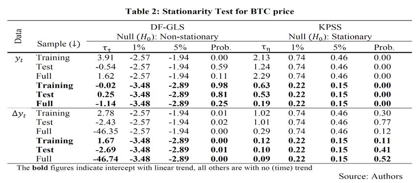
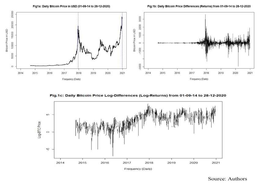
Forecasting with Competing Models…. Adekunle, Gbadebo, Akande, & Adedokun

but no seasonal component HWF ( [False]). We estimate , , and (Table 3), compute the MAE (Table
4) and present plots for 730-step-ahead predictions (Fig.4a – 4g). Some papers (Brügner, 2017) applied
the Holt-winters method.

Forecast Accuracy
The mean absolute error (MAE) is adopted to judge the best prediction technique when we run the
predictions. We use the values of the forecast to evaluate predictions with the historic data from the
same period. The model with the least minimum errors is considered as the best prediction model.
 
 MAE = ∑ ( ̂ +ℎ| − ) ⁄ (8)
 
 The measure ( ̂ +ℎ| − ) = is the forecast error, ̂ +ℎ| forecasted price at time , is
the total # of observations. For the HWF, we added two additional predictions – the prediction interval
forecast which provides uncertainty around a single (the fitted) value, i.e., the upper limit HWF( [0,1];
upper) and the lower limit HWF( [0,1]; lower). The HWF is done at 5% precision level. In all, we
obtain forecast for 18 predictive models. Before we compute the MAE and determine which model best
predict the Bitcoin price, we arbitrarily divided the actual daily Bitcoin data into training-sample (in-
sample) and test-sample (out-sample) periods. In line with Munim et al. (2019), we consider predictions
for the two different training-samples and tests-samples.
 We apply a library(forecast) and library(fpp) in RStudio software for the estimation. The R
programme reports ARIMA(p, d, q), but we follow textbook liturgy and report our result as
ARIMA(p,q,d) earlier defined. For the ARIMA(auto) model, the auto.arima() function returns the best
ARIMA model, based on either Akaike Information Criterion (AIC), corrected Akaike Information
Criterion (AICc) or Bayesian information criterion (BIC) value. The estimation is done with log-
likelihood (LL) method. We adopt Autocorrelation Function (ACF) and Partial Autocorrelation
Function (PACF) to decide the parameter (p,q,d) for the ARIMA(fix) model. We employ the
HoltWinter() function to obtain the parameters of HWF. The HoltWinter() [*, *] reports upper and lower
limits, based on the predictions interval.

Data
We use daily closing price of Bitcoin between 01 Sept., 2014 and 28 Dec., 2020. This period is chosen
putting into consideration the large volume of transactions in the bitcoin and the pattern of price
movements that occurred during these dates. Unlike some machine learning studies (McNally et al.,
2018; Mallqui, 2019) that show forecast for bitcoin returns, we focus on bitcoin price according to
Munim et al. (2019). We filter the daily series and eliminate data for leap years (29\02\2016 and
29\02\2020) which may interruption the consistency and unification of data frequency of 365/year
during estimation. The data which covers 2309 days is sourced from Blockchain.com (01\09\2014 –
14\09\2014) and Finance.yahoo.com (15\09\2014 – 28\12\20).

 Results
Statistical Description
Fig.1a shows the plot of daily bitcoin price, (full sample). The price hits above $700 in 2014 but
would later fall. In same year a leading Bitcoin exchanges (Mt. Gox) which controls about 70%
transactions globally was reportedly hacked and a total of 850,000 BTCs own by customers were stolen.
The exchange suspended trading activities and the incident pose lack of confidence on the security of
Bitcoin exchange. Hence, the price dropped and stood at $434 at 2015 end. Bitcoin experience
spectacular price increase in 2017 to an all-time high of $19,483.06 on 18 December, 2017, but later
dropped to $12,616.64 on Dec., 23. The price decline continued during 2018 and 2019 below its 2017
peak, but experience a full recovery from previous peak by Dec., 2020. The price has shown a trajectory
path of a close reverse L-shape pattern between 2014 and 2018. The shape would later turn an omega
 – an indication of drastic fall and recovery between 2017 peak and Dec., 2020. A cursory look at the
plot shows the data may not be stationary, as would be later confirmed. The plots of difference (Fig.1b)
and log-differences (Fig.1c) show large volatility clustering around zero with notable outliers.

 277 Journal of Studies in Social Sciences and Humanities,2022,8(2), 272-287, E-ISSN: 2413-9270

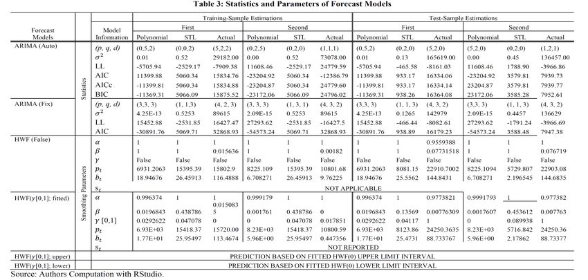
Forecasting with Competing Models…. Adekunle, Gbadebo, Akande, & Adedokun

 Table 1 presents the statistical properties of Bitcoin price data. The standard deviations of the
price indicate higher spread in the full sample than in the training and test samples. The distributions of
all the series are asymmetric (positively skewed), although the full sample is less skewed as compare
to the sub-samples. Both the test-sample and full-sample appear to be mesokurtic (moderately peaked),
while the training sample is leptokurtic (high peaked). The Jarque-Bera values for all series are
significant, rejecting the normality null.
 We observe that the ERS test statistics for the training dataset confusingly signals stationarity,
but this was dislodged when linear trend was incorporated. The statistics suggest we accept the
test null of non-stationarity since ττ > , with or without trends inclusion in the test equation. With
the all the KPSS, we reject the test null of stationarity as the test are highly significance at 1%. Hence,
all results confirm non-stationarity for the training-, test- and full sample for all data frequencies. For
the first difference series of bitcoin price, we reject the null (of non-stationarity) for the DF-GLS test,
and accept the null of stationarity for the KPSS test, both at 1% and 5%. This indicates the bitcoin price
is integrated order of one, I(1).

Generalise (Polynomial and STL) Functions
The actual series depicted by Fig.1a looks chaotic, and for prediction purpose we estimate the
polynomial and STL functions. For the polynomial model, we obtain 0 = 7.784e+08, 1 =
− 7.741e+05 and 2 =1.925e+02. The fitted values, ̂ =7.784e+08− 7.741e+05 + 1.925e+02 2 ,
was plotted (the purple line in Fig.3a) which would be later use for predictions. Fig.2 shows how the
SLT decompose the actual data (topmost graph) into key time-series components. We observe that the
trend is explosives, the remainder is convergence and mean reversing, and the seasonality is both
oscillatory and stable around it zero mean. For STL split, we adopt the STL Trend (third line) for
prediction purpose.
 Figure 3a shows a plot of the Actual data, STL-Trend and Polynomial function of BTC price.
The actual function looks chaotic, nonlinear with spiky striations. The Polynomic function is so general
and simple that its prediction smooths the actual data. For nonlinear series, Lahmiri et al. (2018) suggest
a log-transformed comparism to obtain suitable estimates. Figure 3b presents an analogous logarithmic
transformation plot. Unlike the level form and as it would be expected, the log-transformation exhibits
similar nonlinear but relative smooth striations with protrusions in periods of price peaks.

Estimated ARIMA and HWF Models
The study aims to find a model that enables more accurate prediction of daily bitcoin price. To do this,
we find the order of the ARIMA model and the HWF optimal smoothing parameters for the forecast
models. The Table 3 shows the appropriate order chosen for the Polynomial, STL and Actual series are
ARIMA(0,5,2), ARIMA(0,0,2) and ARIMA(5,2,2), respectively. These orders are applied to construct
the ARIMA forecast models and for the prediction of the three Bitcoin price functions. These HWF
parameters, , and are presented for the STL, Polynomial and Actual functions. The parameter
would be applied to construct the Holt-Winters models and predict Bitcoin price for 730 days, until 27-
12-2023. The forecast interval is shown for the polynomial, STL-trend and Actual data.

 278 Journal of Studies in Social Sciences and Humanities,2022,8(2), 272-287, E-ISSN: 2413-9270

Forecasting with Competing Models…. Adekunle, Gbadebo, Akande, & Adedokun

 279 Journal of Studies in Social Sciences and Humanities,2022,8(2), 272-287, E-ISSN: 2413-9270

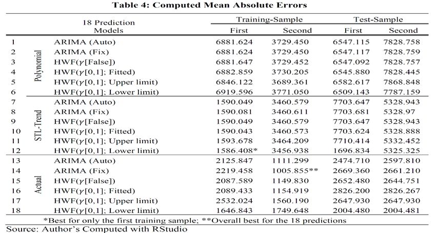
Forecasting with Competing Models…. Adekunle, Gbadebo, Akande, & Adedokun

 Discussions
We check the model’s performance and decide the model suitable for predicting the Bitcoin price. For
cross-validation, we arbitrarily split the actual Bitcoin data into two different training-samples and test-
samples. While there is no theoretical underpinning in choosing the sample duration, we are concern
about the pattern the bitcoin plots (Fig.1a) formed overtime. We introspect the pattern formed choose
the periods from 01\09\14 to 18\12\17 (1205 days) as first training-sample. The first test-sample data
range from 19\12\17 – 28\12\2020, with 1104 days. The second training-sample is considered from
01\09\14 to 30\06\19 (1764 days), with test-sample data set of 01\07\19 – 28\12\2020 (545 days). We
compare the computed MAE for 18 models, and adjudge the one with the least MAE as best predictor.
Table 4 shows that although the HWF( [0,1]; lower-limit) for the STL-trend provides the best
prediction on the first training-sample with the smallest MAE of $1586.408, but the MAE of $1005.855
for the ARIMA on the actual function outperform it in the second training-sample. The discussion show
that the Holt-Winters model is more appropriate for prediction of the daily bitcoin price with STL-trend
as the time series, while ARIMA(fix) model provide more accurate when actual data is applied.
 Fig. 4a-4g show the predictions for the models. The black lines represent actual data function,
red represents the STL-Trend, and purple represents the polynomial function. Each prediction line is
identified by the legend on the plots. The other two variants of green lines “yellow green” and “green4”
are for the HWF( [0,1]; upper limit) and HWF( [0,1]; lower limit) prediction interval, respectively.
Fig.4a shows the predictions for the polynomial function. The plot shows that with the polynomial
series, the predictions are closed within similar interval with little precisions. The various prediction is
within regions that are not too different from each other. The predictions are closed because the
polynomial function is very general, simple and hence influence the prediction with similar techniques.
This changes when same prediction models are applied for STL-Trend and Actual function. Fig. 4b and
4c present predictions for the STL-Trend based and Actual function, respectively. Both plots show
quite different predictions values for the future with larger variability for the predictions when compare
with Fig 4a. Fig. 4d, 4f and 4g, respectively show plots for all predictions in level form with predictions
interval (shaded regions) based on actual, polynomial and STL-trend functions of the bitcoin price.
Fig.4e show plot for predictions for log-transform with predictions based on STL-trend function of the
full-sample of the Bitcoin price.

 280 Journal of Studies in Social Sciences and Humanities,2022,8(2), 272-287, E-ISSN: 2413-9270

Forecasting with Competing Models…. Adekunle, Gbadebo, Akande, & Adedokun

 281 Journal of Studies in Social Sciences and Humanities,2022,8(2), 272-287, E-ISSN: 2413-9270

Forecasting with Competing Models…. Adekunle, Gbadebo, Akande, & Adedokun

 282 Journal of Studies in Social Sciences and Humanities,2022,8(2), 272-287, E-ISSN: 2413-9270

Forecasting with Competing Models…. Adekunle, Gbadebo, Akande, & Adedokun

 Implications
 The study predicts daily bitcoin prices using observed data, and datasets from constructed
generalise functions based on pattern exhibited by the price fluctuations. Because of markets
information asymmetric, increasing economic uncertainties, erratic behaviours of cryptocurrency
miners and other markets dynamics, adopting a predictive model to understand the directions and
possible predictable value of Bitcoins is important. Hence, the findings of this study have some
significant implications for Bitcoin, cryptocurrency and general financial markets, as well as for
research in the field of empirical finance.
 First, the results provide guide for investors to make informed decisions when considering
investment in the cryptocurrency market given the excessive volatile nature of Bitcoin. Accurate
predictions minimize potential losses-risks for investors, traders and users. Bitcoin has attracted
stakeholders, including individual and institutional investors since its inventions. We suppose that the
model completed offer best accurate price forecasts for Bitcoin. Second, the forecast models has
implications to drive asset allocations. Our optimal model offers warnings signals to financial markets
investors in order circumvent massive losses from sporadic volatility in the price. Asset managers may
want to avoid potential risk by adopting least error forecast models to predict likely direction and value
of the Bitcoin price. Since Bitcoin is now becoming save haven, and possible substitute for other
traditional assets, and commodities (Kliber et al., 2019), the predictive models. Lastly, the findings offer
significant implication in empirical finance, particularly to researchers interested in the bitcoin and
cryptocurrency. Extant attempt at Bitcoin price predictions focused on the use of observed data. Actual
data is too noisy and increases the risk of inaccurate predictions. Hence, a generalised function
transformation offers better predictions as our result supposed. Our functions can be applied to construct
hybrid models for future price forecast.

 Conclusions
 The sporadic nature of Bitcoin price has prompted attempts to forecast its daily future price
(Munim et al.., 2019; Chen et al., 2020; Hung et al., 2020). We establish accurate forecast models that
better predict the price of Bitcoin. The is done by considering the model with the least value of MAE
for the actual daily bitcoin price, and two generalised (polynomial and STL) functions adopted to
forecast the time-series. We establish that although the Holt-Winters Filter with trend and additive
seasonality use on the STL-trend HWF( [0,1]; lower limit) provides the best prediction on the first
training-sample with the smallest MAE of 1586.408, but when validated with the MAE of 1005.855 of
the ARIMA(fix) model applied on the Actual function in the second training-sample, the later
outperform the former. The results show that the Holt-Winters model is more appropriate for prediction
of the daily price of Bitcoin with STL-trend as the time-series, while ARIMA(fix) model provide more
accurate when actual data is applied. This finding would serve as a guide to investors, traders, regulators
and other participants in the cryptocurrency market.
 283 Journal of Studies in Social Sciences and Humanities,2022,8(2), 272-287, E-ISSN: 2413-9270

Forecasting with Competing Models…. Adekunle, Gbadebo, Akande, & Adedokun

 References
Adcock, R., & Gradojevic, N. (2019). Non-fundamental, non-parametric Bitcoin forecasting. Physica A:
 Statistical Mechanics and Its Applications, 531, 121727.
 https://doi.org/10.1016/j.physa.2019.121727
Atsalakis, G. S., Atsalaki, I. G., Pasiouras, F., & Zopounidis, C. (2019). Bitcoin price forecasting with
 neuro-fuzzy techniques. European Journal of Operational Research, 276(2), 770–780.
 https://doi.org/10.1016/j.ejor.2019.01.040
Aygün, B., & Günay Kabakçı, E. (2021). Comparison of statistical and machine learning algorithms for
 forecasting daily bitcoin returns. European Journal of Science and Technology, 21, 444–454.
 https://doi.org/10.31590/ejosat.822153
Basher, S. A., & Sadorsky, P. (2022). Forecasting Bitcoin price direction with random forests: How
 important are interest rates, inflation, and market volatility? MPRA, Paper No. 113293. Available
 at: https://mpra.ub.uni-muenchen.de/113293/MPRA
Baur, D. G., Hong, K., & Lee, A. (2018). Bitcoin: Medium of exchange or speculative assets? J. of Int.
 Fin. Markets, Institutions & Money, 54, 177 – 189. https://doi.org/10.1016/j.intfin.2017.12.004
Baur, D., Cahill, D., Godfrey, K., & Liu, Z. (2019). Bitcoin time-of-day, day-of-week and month-of-year
 effects in returns and trading volume. Finance Res. Letters. 31, 78–92.
 https://doi.org/10.1016/j.frl.2019.04.023
Box, G. E. P., & Jenkins, G. M. (1976). Time Series Analysis: forecasting and control. Revised ed. San
 Francisco: Holden-Day . https://doi.org/10.2307/2284112
Brügner, H. (2017). Holt-Winters traffic prediction on aggregated flow data: seminars FI / IITM SS 17,
 Network Architectures and Services. https://doi.org/10.2313/NET-2017-09-1_04
Caporale, G. M., Gil-Alana, L., & Plastun, A. (2018). Persistence in the cryptocurrency market. Research
 in International Business and Finance, 46, 141 – 48. https://doi.org/10.1016/j.ribaf.2018.01.002
Chen, Z., Li, C., & Sun, W. (2020). Bitcoin price prediction using machine learning: An approach to
 sample dimension engineering. Journal of Computational and Applied Mathematics, 365,
 112395. https://doi.org/10.1016/j.cam.2019.112395
Chowdhury, A., & Mendelson, B. K. (2014). Virtual currency and the financial system: The case of
 Bitcoin. Dept. of Economics, College of Business Administration, Marquette.. Finance Research
 Letters, 26, 81 – 88. https://doi.org/10.1016/j.frl.2017.12.006
Demir, A., Akılotu, B.N., Kadiroğlu, Z., & Sengür, A. (2019). Bitcoin price prediction using machine
 learning methods. In Proceedings of the 2019 1st International Informatics and Software
 Engineering Conference (UBMYK), Ankara, Turkey, 6–7 November 2019.
 https://doi.org/10.1109/UBMYK48245.2019.8965445
Elliott, G., Rothenberg, T.J., & Stock, J.H. (1996). Efficient tests for an autoregressive unit root.
 Econometrica 64, 813 – 836. https://doi.org/10.2307/2171846
Gbadebo, A. D., Adekunle, A. O., Adedokun, W. Lukman, A. A., & Akande, J. O. (2021). BTC price
 volatility: Fundamentals versus information. Cogent Business & Management, 8(1).
 https://doi.org/10.1080/23311975.2021.1984624
Goutte, S., Guesmi, K., & Saadi, S. (2019). Cryptofinance and mechanisms of exchange: the making of
 virtual currency. Springer Edition. ISBN 978-3-030-30738-7. Available at:
 https://link.springer.com/book/10.1007/978-3-030-30738-7
Guizani, S., & Nafti I. K. (2019). The determinants of Bitcoin price volatility: an investigation with ARDL
 Model. Procedia Computer Science, 164, 233 – 238. https://doi.org/10.1016/j.procs.2019.12.177.
Hamayel, M. J., & Owda, A. Y. (2021). A novel cryptocurrency price prediction model using GRU,
 LSTM and bi-LSTM Machine Learning Algorithms. AI, 2(4), 477–496.
 https://doi.org/10.3390/ai2040030
Holt, C. C. (1957). Forecasting trends and seasonals by exponentially weighted moving averages. ONR
 Research Memorandum, 52. https://doi.org/10.1016/j.ijforecast.2003.09.015
Hung, J., Liu, H., & Yang, J. C (2020). Improving the realized GARCH’s volatility forecast for Bitcoin
 with jump-robust estimators. North American Journal of Economics and Finance. 52, 101–165,
 https://doi.org/10.1016/j.najef.2020.101165
Hyndman, R. J., & Athanasopoulos, G. (2018). Forecasting: principles and practice, 2nd ed. OTexts,
 Melbourne, Australia. Available at: https://otexts.com/fpp2
 284 Journal of Studies in Social Sciences and Humanities,2022,8(2), 272-287, E-ISSN: 2413-9270

Forecasting with Competing Models…. Adekunle, Gbadebo, Akande, & Adedokun

Jang, H., & Lee, J. (2018). An empirical study on modeling and prediction of bitcoin prices with Bayesian
 neural networks based on blockchain information. IEEE Access, 6, 5427–5437.
 https://doi.org/10.1109/ACCESS.2017.2779181
Jaquart, P., Dann, D., & Weinhardt, C. (2021). Short-term bitcoin market prediction via machine learning.
 J. of Finance and Data Science, 7, 45–66. https://doi.org/10.1016/j.jfds.2021.03.001
Jeon, Y., Samarbakhsh, L., & Hewitt, K. (2020). Fragmentation in the Bitcoin market: Evidence from
 multiple coexisting order books. Finance Research Letters.
 https://doi.org/10.1016/j.frl.2020.101654
Kliber, A., Marszałek, P., Musiałkowska, I., & Świerczyńska, K. (2019). Bitcoin: Safe haven, hedge or
 diversifier? Perception of bitcoin in the context of a country’s economic situation—A stochastic
 volatility approach. Physica A: Statistical Mechanics and Its Applications, 524, 246–257.
 https://doi.org/10.1016/j.physa.2019.04.145
Kundra, H., Sharma, S., Nancy, P. and Kalyani, D. (2022). A two level ensemble classification approach
 to forecast bitcoin prices. Kybernetes, https://doi.org/10.1108/K-11-2021-1213
Kwiatkowski, D., Phillips, P.C.B., Schmidt, P., Shin, Y. (1992). Testing the null hypothesis of stationarity
 against an alternative of a unit root. Journal Econometrica. 54: 159 – 178.
 https://doi.org/10.1016/0304-4076(92)90104-Y
Kyriazis, N. A. (2020). Is Bitcoin Similar to Gold? An integrated overview of empirical findings. Journal
 of Risk and Financial Management, 13(5), 88. https://doi.org/10.3390/jrfm13050088
Lahmiri, S., & Bekiros, S. (2020) Intelligent forecasting with machine learning trading systems in chaotic
 intraday Bitcoin market. Chaos Solitons Fractals, 133, 109641.
 https://doi.org/10.1016/j.chaos.2020.109641
Lahmiri, S., Bekiros, S., & Salvi, A. (2018). Long-range memory, distributional variation and randomness
 of Bitcoin volatility. Chaos, Solitons and Fractals 107, 43 – 48.
 https://doi.org/10.1016/j.chaos.2017.12.018
Rizwan, M., Narej, S., & Javed, M. Bitcoin price prediction using deep learning algorithm. 2019 13th
 International Conference on Mathematics, Actuarial Science, Computer Science and Statistics,
 1-7, https://doi.org/10.1109/MACS48846.2019.9024772
Mallqui, D. C., & Fernandes, R. A. (2019). Predicting the direction, maximum, minimum and closing
 prices of daily Bitcoin exchange rate using machine learning techniques. Application of Software
 Computer, 75:596 – 606. https://doi.org/10.1016/j.asoc.2018.11.038
McNally, S., Roche, J., & Caton, S. (2018). Predicting the price of Bitcoin using machine learning. In:
 Proceedings - 26th Euromicro International Conference on Parallel, Distributed, and Network
 Based Processing, pp 339 – 343. https://doi.org/10.1109/PDP2018.2018.00060
Mudassir, M., Bennbaia, S., Unal, D., & Hammoudeh, M. (2020). Time-series forecasting of Bitcoin
 prices using high-dimensional features: A machine learning approach. Neural Computing and
 Applications. https://doi.org/10.1007/s00521-020-05129-6
Munim, Z. H., Shakil, M. H., & Alon, I. (2019). Next-day Bitcoin price forecast. Journal of Risk Financial
 Management, 12, 103 – 120. https://doi:10.3390/jrfm12020103
Pabuçcu, H., Ongan, S., & Ongan, A. (2020). Forecasting the movements of Bitcoin prices: An application
 of machine learning algorithms. Quantitative Finance and Economics, 4(4), 679–692.
 https://doi.org/10.3934/QFE.2020031
Troster, V., Tiwari, A. K., Shahbaz, M., & Macedo, D. N. (2019). Bitcoin returns and risk: A general
 GARCH and GAS analysis. 30(C), 187–193. https://doi.org/10.1016/j.frl.2018.09.014
Urquhart, A. (2018). What causes the attention of Bitcoin? Economics Letter. 166, 40–44.
 https://doi.org/10.1016/j.econlet.2018.02.017
Velankar, S., Valecha, S., & Maji, S. Bitcoin Price Prediction using Machine Learning. In Proceedings of
 the 20th International Conference on Advanced Communications Technology (ICACT),
 Chuncheon-si, Korea, 11–14, February 2018. https://doi.org/10.23919/ICACT.2018.8323676.
Winters, P. R. (1960). Forecasting sales by exponentially weighted moving averages. Management
 Science, 6, 324 – 342. https://doi.org/10.1287/mnsc.6.3.324
Ye, Z., Wu, Y., Chen, H., Pan, Y., & Jiang, Q. 2022. A stacking ensemble deep learning model for bitcoin
 price prediction using twitter comments on Bitcoin. Mathematics.
 https://doi.org/10.3390/math10081307

 285 Journal of Studies in Social Sciences and Humanities,2022,8(2), 272-287, E-ISSN: 2413-9270

Forecasting with Competing Models…. Adekunle, Gbadebo, Akande, & Adedokun

 Appendix
R Scripts
read.csv("BTC.csv", header= T) #Read in data
BTC

Forecasting with Competing Models…. Adekunle, Gbadebo, Akande, & Adedokun

 {
 mae[1,i]