A universal velocity profile for turbulent wall flows including adverse pressure gradient boundary layers

Page created by Frances Harmon
 
CONTINUE READING
A universal velocity profile for turbulent wall flows including adverse pressure gradient boundary layers
Downloaded from https://www.cambridge.org/core. IP address: 46.4.80.155, on 07 Jan 2022 at 19:03:55, subject to the Cambridge Core terms of use, available at https://www.cambridge.org/core/terms. https://doi.org/10.1017/jfm.2021.998

                                                                                                                                                                                                                                           J. Fluid Mech. (2022), vol. 933, A16, doi:10.1017/jfm.2021.998

                                                                                                                                                                                                                                           A universal velocity profile for turbulent wall
                                                                                                                                                                                                                                           flows including adverse pressure gradient
                                                                                                                                                                                                                                           boundary layers

                                                                                                                                                                                                                                           Matthew A. Subrahmanyam1, †, Brian J. Cantwell1 and Juan J. Alonso1
                                                                                                                                                                                                                                           1 Department   of Aeronautics and Astronautics, Stanford University, Stanford, CA 94305, USA

                                                                                                                                                                                                                                           (Received 9 June 2021; revised 26 October 2021; accepted 6 November 2021)

                                                                                                                                                                                                                                           A recently developed mixing length model of the turbulent shear stress in pipe flow
                                                                                                                                                                                                                                           is used to solve the streamwise momentum equation for fully developed channel flow.
                                                                                                                                                                                                                                           The solution for the velocity profile takes the form of an integral that is uniformly valid
                                                                                                                                                                                                                                           from the wall to the channel centreline at all Reynolds numbers from zero to infinity.
                                                                                                                                                                                                                                           The universal velocity profile accurately approximates channel flow direct numerical
                                                                                                                                                                                                                                           simulation (DNS) data taken from several sources. The universal velocity profile also
                                                                                                                                                                                                                                           provides a remarkably accurate fit to simulated and experimental flat plate turbulent
                                                                                                                                                                                                                                           boundary layer data including zero and adverse pressure gradient data. The mixing length
                                                                                                                                                                                                                                           model has five free parameters that are selected through an optimization process to provide
                                                                                                                                                                                                                                           an accurate fit to data in the range Rτ = 550 to Rτ = 17 207. Because the velocity profile is
                                                                                                                                                                                                                                           directly related to the Reynolds shear stress, certain statistical properties of the flow can be
                                                                                                                                                                                                                                           studied such as turbulent kinetic energy production. The examples presented here include
                                                                                                                                                                                                                                           numerically simulated channel flow data from Rτ = 550 to Rτ = 8016, zero pressure
                                                                                                                                                                                                                                           gradient (ZPG) boundary layer simulations from Rτ = 1343 to Rτ = 2571, zero pressure
                                                                                                                                                                                                                                           gradient turbulent boundary layer experimental data between Rτ = 2109 and Rτ = 17 207,
                                                                                                                                                                                                                                           and adverse pressure gradient boundary layer data in the range Rτ = 912 to Rτ = 3587.
                                                                                                                                                                                                                                           An important finding is that the model parameters that characterize the near-wall flow do
                                                                                                                                                                                                                                           not depend on the pressure gradient. It is suggested that the new velocity profile provides
                                                                                                                                                                                                                                           a useful replacement for the classical wall-wake formulation.
                                                                                                                                                                                                                                           Key words: turbulence modelling, turbulence theory, turbulent boundary layers

                                                                                                                                                                                                                                                                 † Email address for correspondence: msubrahm@stanford.edu
                                                                                                                                                                                                                                           © The Author(s), 2021. Published by Cambridge University Press. This is an Open Access article,
                                                                                                                                                                                                                                           distributed under the terms of the Creative Commons Attribution licence (https://creativecommons.
                                                                                                                                                                                                                                           org/licenses/by/4.0/), which permits unrestricted re-use, distribution, and reproduction in any medium,
                                                                                                                                                                                                                                           provided the original work is properly cited.                                                             933 A16-1
A universal velocity profile for turbulent wall flows including adverse pressure gradient boundary layers
Downloaded from https://www.cambridge.org/core. IP address: 46.4.80.155, on 07 Jan 2022 at 19:03:55, subject to the Cambridge Core terms of use, available at https://www.cambridge.org/core/terms. https://doi.org/10.1017/jfm.2021.998

                                                                                                                                                                                                                                                              M.A. Subrahmanyam, B.J. Cantwell and J.J. Alonso
                                                                                                                                                                                                                                           1. Introduction
                                                                                                                                                                                                                                           We are concerned with approximating incompressible wall-bounded flows including
                                                                                                                                                                                                                                           several examples of channel flow and wall boundary layers, as sketched in figure 1. These
                                                                                                                                                                                                                                           flows are governed by the two-dimensional, stationary, Reynolds-averaged Navier–Stokes
                                                                                                                                                                                                                                           (RANS) equations (1.1a,b):

                                                                                                                                                                                                                                                 ∂           ∂   1 ∂p           ∂ 2 ui            ∂uj
                                                                                                                                                                                                                                                    ui uj +     ui uj +       −ν         = 0,           = 0,       (i, j) = (1, 2).   (1.1a,b)
                                                                                                                                                                                                                                                ∂xj         ∂xj         ρ ∂xi    ∂xj ∂xj            ∂xj

                                                                                                                                                                                                                                             At high Reynolds number, the flow over a flat plate is accurately described by the
                                                                                                                                                                                                                                           boundary layer approximation,

                                                                                                                                                                                                                                               ∂        ∂      ∂            1 dpe (x)    ∂ 2u                      ∂u ∂v
                                                                                                                                                                                                                                                  (uu) + (uv) + (u v  ) +           − ν 2 = 0,                      +    = 0,       (1.2a,b)
                                                                                                                                                                                                                                               ∂x       ∂y     ∂y           ρ dx         ∂y                        ∂x   ∂y
                                                                                                                                                                                                                                           subject to the no-slip condition at the wall and the free-stream velocity at the outer edge
                                                                                                                                                                                                                                           of the boundary layer,
                                                                                                                                                                                                                                                                         u(0) = v(0) = 0,         u (δh ) = ue .                      (1.3a,b)
                                                                                                                                                                                                                                           The boundary layer thickness in figure 1 is denoted δh as is the channel half-height. The
                                                                                                                                                                                                                                           reason for this is described in detail by Cantwell (2021) and will be discussed further in § 5,
                                                                                                                                                                                                                                           where the universal velocity profile will be used to define an equivalent channel half-height
                                                                                                                                                                                                                                           for the boundary layer. This establishes a practically useful, unambiguous, measure of the
                                                                                                                                                                                                                                           overall boundary layer thickness. In fully developed channel flow, all dependence on x
                                                                                                                                                                                                                                           vanishes, the flow is parallel and the governing equations of motion reduce to

                                                                                                                                                                                                                                                                         ∂   1 dpe (x)    ∂ 2u
                                                                                                                                                                                                                                                                            uv +         − ν 2 = 0,                                      (1.4)
                                                                                                                                                                                                                                                                         ∂y      ρ dx       ∂y
                                                                                                                                                                                                                                           where pe is the channel pressure, independent of height above the wall, and the pressure
                                                                                                                                                                                                                                           gradient is an externally imposed constant.
                                                                                                                                                                                                                                             At Reynolds numbers large enough to produce turbulence, the no-slip condition imposed
                                                                                                                                                                                                                                           by viscosity leads to an array of highly unsteady, three-dimensional, streamwise-aligned
                                                                                                                                                                                                                                           eddies adjacent to the wall. The intense vortical motion associated with these eddies
                                                                                                                                                                                                                                           generates very strong convective and viscous wall-normal transport of x-momentum.
                                                                                                                                                                                                                                           The average effect of this balance of viscous and convective stresses is to produce a
                                                                                                                                                                                                                                           well-defined wall layer with a very steep mean velocity gradient at the wall over a length
                                                                                                                                                                                                                                           scale comparable to the scale of the eddies just described. The mean velocity variation
                                                                                                                                                                                                                                           over this wall layer scales with the friction velocity,
                                                                                                                                                                                                                                                                                                1/2
                                                                                                                                                                                                                                                                                            τw
                                                                                                                                                                                                                                                                                 uτ =                   .                                (1.5)
                                                                                                                                                                                                                                                                                            ρ
                                                                                                                                                                                                                                           Above the wall layer, viscous stresses become small and momentum transport is dominated
                                                                                                                                                                                                                                           by turbulent eddying motions over a length scale comparable to the thickness of the
                                                                                                                                                                                                                                           boundary layer. The large-scale eddies produce wall-normal convection of the turbulence
                                                                                                                                                                                                                                           generated close to the wall in a manner that can be compared with the smoothing out of
                                                                                                                                                                                                                                           the momentum deficit of a plane wake. The velocity variation over this outer wake layer
                                                                                                                                                                                                                                           scales with the aptly named defect velocity (ue − uτ ).
                                                                                                                                                                                                                                           933 A16-2
A universal velocity profile for turbulent wall flows including adverse pressure gradient boundary layers
Downloaded from https://www.cambridge.org/core. IP address: 46.4.80.155, on 07 Jan 2022 at 19:03:55, subject to the Cambridge Core terms of use, available at https://www.cambridge.org/core/terms. https://doi.org/10.1017/jfm.2021.998

                                                                                                                                                                                                                                                               A universal velocity profile for turbulent wall flows
                                                                                                                                                                                                                                               (a)                                                (b)

                                                                                                                                                                                                                                                                                                                   ue (x)
                                                                                                                                                                                                                                                 2δh                         ue
                                                                                                                                                                                                                                                           y
                                                                                                                                                                                                                                                                                                                            δh (x)

                                                                                                                                                                                                                                                                                                                                         x
                                                                                                                                                                                                                                                                Figure 1. Channel and flat plate flows with nomenclature.

                                                                                                                                                                                                                                           2. The wall-wake formulation
                                                                                                                                                                                                                                           While there is no first-principles theory that leads to the turbulent boundary layer velocity
                                                                                                                                                                                                                                           profile, the wall-wake formulation introduced by Coles (1956) in his landmark paper
                                                                                                                                                                                                                                           provides a very good correlation that accurately reflects the relative balance between
                                                                                                                                                                                                                                           viscous and turbulent stresses across most of the layer and can be used to compare flows at
                                                                                                                                                                                                                                           different Reynolds numbers. In this formulation, the y-coordinate and streamwise velocity
                                                                                                                                                                                                                                           are normalized using friction variables
                                                                                                                                                                                                                                                                                         uτ y               u
                                                                                                                                                                                                                                                                                  y+ =        ,     u+ =       .                       (2.1a,b)
                                                                                                                                                                                                                                                                                          ν                 uτ
                                                                                                                                                                                                                                           The friction Reynolds number, sometimes called the Kármán number and sometimes
                                                                                                                                                                                                                                           denoted δ + , is the y+ coordinate evaluated at δh ,
                                                                                                                                                                                                                                                                                                  uτ δh
                                                                                                                                                                                                                                                                                     Rτ =               .                                 (2.2)
                                                                                                                                                                                                                                                                                                   ν
                                                                                                                                                                                                                                           Here, Rτ will be the primary measure of flow Reynolds number in this paper. There is
                                                                                                                                                                                                                                           a lower limit, Rτ ≈ 100, below which wall turbulence cannot be sustained (Schlichting &
                                                                                                                                                                                                                                           Gersten 2000, p. 535), whereas the highest Reynolds number laboratory wall flows studied
                                                                                                                                                                                                                                           to date can reach Rτ > 500 000 while geophysical flows can reach much higher values. In
                                                                                                                                                                                                                                           this range, u+ at the outer edge of the boundary layer, u+ = ue /uτ , varies from a low of
                                                                                                                                                                                                                                           approximately 15 to a high close to 40 or more.
                                                                                                                                                                                                                                              At the wall, the velocity profile is linear, τw /ρ = ν∂u/∂y = νu/y, and to a good
                                                                                                                                                                                                                                           approximation,
                                                                                                                                                                                                                                                                                           u+ =y+                                         (2.3)
                                                                                                                                                                                                                                           within the so-called viscous sublayer, (0 < y+  5). The Coles wall-wake profile given
                                                                                                                                                                                                                                           by
                                                                                                                                                                                                                                                                                                   +
                                                                                                                                                                                                                                                                         1              Π (x)     y
                                                                                                                                                                                                                                                                    u+ = ln y+ + C +            W                            (2.4)
                                                                                                                                                                                                                                                                         κ                  κ       Rτ
                                                                                                                                                                                                                                           is a good approximation in the range (≈ 100 < y+ < Rτ ). The first two terms of (2.4)
                                                                                                                                                                                                                                           comprise the law of the wall introduced by von Kármán (1931). Coles (1956) recommends
                                                                                                                                                                                                                                           k = 0.41 and C = 5.0. The last term in (2.4) is the law of the wake that Coles determined
                                                                                                                                                                                                                                           from a careful study of a variety of flow data for various pressure gradients. The function W
                                                                                                                                                                                                                                           provides the self-similar shape of the velocity profile in the outer flow, while the function
                                                                                                                                                                                                                                           Π is used to change the amplitude of the outer velocity profile to account for the effect of
                                                                                                                                                                                                                                           the pressure gradient. Coles suggested W = 2 sin2 ((π/2)(y/δ)), where y+ /Rτ = y/δ and
                                                                                                                                                                                                                                           δ is the boundary layer thickness, as a good choice for the wake-like shape of the outer
                                                                                                                                                                                                                                                                                                                                     933 A16-3
A universal velocity profile for turbulent wall flows including adverse pressure gradient boundary layers
Downloaded from https://www.cambridge.org/core. IP address: 46.4.80.155, on 07 Jan 2022 at 19:03:55, subject to the Cambridge Core terms of use, available at https://www.cambridge.org/core/terms. https://doi.org/10.1017/jfm.2021.998

                                                                                                                                                                                                                                                                M.A. Subrahmanyam, B.J. Cantwell and J.J. Alonso
                                                                                                                                                                                                                                                                            30
                                                                                                                                                                                                                                                                            25
                                                                                                                                                                                                                                                                            20
                                                                                                                                                                                                                                                                        u+ 15
                                                                                                                                                                                                                                                                            10
                                                                                                                                                                                                                                                                             5
                                                                                                                                                                                                                                                                             0
                                                                                                                                                                                                                                                                              100      101      102      103      104
                                                                                                                                                                                                                                                                                                  y+
                                                                                                                                                                                                                                           Figure 2. Equation (2.5) used by Spalding (1961) to connect the sublayer to the log region. Dashed curve is
                                                                                                                                                                                                                                                                        u+ = y+ . Constants are κ = 0.41 and C = 5.0.

                                                                                                                                                                                                                                           velocity profile. For dpe /dx = 0, Coles used Π = 0.62. The part of the velocity profile
                                                                                                                                                                                                                                           that connects the viscous sublayer (2.3) to the beginning of the law of the wall in (2.4) is
                                                                                                                                                                                                                                           called the buffer layer.
                                                                                                                                                                                                                                             Missing from the theory at that time, and highly sought after by a number of
                                                                                                                                                                                                                                           investigators including Deissler (1954), van Driest (1956) and others, was a single formula
                                                                                                                                                                                                                                           that could span the entire wall layer connecting the viscous sublayer (2.3) through the
                                                                                                                                                                                                                                           buffer layer to the law of the wall. The problem was solved by Spalding (1961), who came
                                                                                                                                                                                                                                           up with the implicit formula,
                                                                                                                                                                                                                                                                  +                       2         3        + 4 
                                                                                                                                                                                                                                                y+ =u+ + e−κC eκu − 1 − κu+ − 12 κu+ − 16 κu+ − 24            1
                                                                                                                                                                                                                                                                                                                  κu     ···      (2.5)

                                                                                                                                                                                                                                           shown in figure 2. Although somewhat awkward to use, this formula asymptotes to the
                                                                                                                                                                                                                                           linear profile at the wall at small u+ and approaches the logarithm as the exponential
                                                                                                                                                                                                                                           term inside the parentheses dominates the algebraic terms for u+ > 30. There are several
                                                                                                                                                                                                                                           features of the Coles wall-wake formulation of the velocity profile that can be noted.
                                                                                                                                                                                                                                             (i) The velocity derivative has a small discontinuity at the outer edge of the boundary
                                                                                                                                                                                                                                                 layer owing to the log term that continues to increase with y+ .
                                                                                                                                                                                                                                            (ii) There is a discontinuity at the matching point between the Spalding and Coles
                                                                                                                                                                                                                                                 profiles where they overlap. At low Reynolds number, the discontinuity becomes
                                                                                                                                                                                                                                                 quite apparent, requiring additional terms to be included in (2.5).
                                                                                                                                                                                                                                           (iii) There is a long running debate as to the validity of the logarithmic dependence of
                                                                                                                                                                                                                                                 the velocity profile outside the viscous wall layer. The profile (2.4) assumes the log
                                                                                                                                                                                                                                                 law.
                                                                                                                                                                                                                                           (iv) The profile is not connected to any model of the turbulent shear stress.

                                                                                                                                                                                                                                           3. The universal velocity profile
                                                                                                                                                                                                                                           Expressing (1.4) in wall normalized coordinates, integrating once and applying the free
                                                                                                                                                                                                                                           stream condition, du+ /dy+ = 0 at y+ = Rτ , the result is
                                                                                                                                                                                                                                                                                              
                                                                                                                                                                                                                                                                        +     du+           y+
                                                                                                                                                                                                                                                                       τ + + − 1−                  = 0,                      (3.1)
                                                                                                                                                                                                                                                                              dy            Rτ

                                                                                                                                                                                                                                           where τ + = −u v  /(uτ )2 . This equation is identical to the governing stress balance in
                                                                                                                                                                                                                                           pipe flow. This fact motivated Subrahmanyam, Cantwell & Alonso (2021) to approximate
                                                                                                                                                                                                                                           velocity profiles in channel flow and the zero pressure gradient boundary layer using the
                                                                                                                                                                                                                                           933 A16-4
A universal velocity profile for turbulent wall flows including adverse pressure gradient boundary layers
Downloaded from https://www.cambridge.org/core. IP address: 46.4.80.155, on 07 Jan 2022 at 19:03:55, subject to the Cambridge Core terms of use, available at https://www.cambridge.org/core/terms. https://doi.org/10.1017/jfm.2021.998

                                                                                                                                                                                                                                                               A universal velocity profile for turbulent wall flows
                                                                                                                                                                                                                                           same universal velocity profile used by Cantwell (2019) to approximate the Princeton
                                                                                                                                                                                                                                           Superpipe (PSP) data (Zagarola 1996; Zagarola & Smits 1998; Jiang, Li & Smits 2003;
                                                                                                                                                                                                                                           McKeon 2003).
                                                                                                                                                                                                                                             In this approach, the shear stress is modelled using classical mixing length theory (von
                                                                                                                                                                                                                                           Kármán 1931; Prandtl 1934; van Driest 1956),
                                                                                                                                                                                                                                                                                               
                                                                                                                                                                                                                                                                                        du+ 2
                                                                                                                                                                                                                                                                             τ + = λ y+             ,                            (3.2)
                                                                                                                                                                                                                                                                                            dy+
                                                                                                                                                                                                                                           where λ( y+ ) is the mixing length function. When (3.2) is substituted into (3.1), the result
                                                                                                                                                                                                                                           is a quadratic equation for du+ /dy+ . We use the positive root
                                                                                                                                                                                                                                                                                                                 1/2
                                                                                                                                                                                                                                                         du+           1           1                + 2        y+
                                                                                                                                                                                                                                                               = −           +             1 + 4λ( y  )    1 −          .          (3.3)
                                                                                                                                                                                                                                                          dy+       2λ( y+ )2 2λ( y+ )2                        Rτ
                                                                                                                                                                                                                                           Equation (3.3) is integrated from the wall to y+ to obtain the velocity profile in the form
                                                                                                                                                                                                                                           of an integral dependent on the non-dimensional mixing length λ( y+ ) and Rτ ,
                                                                                                                                                                                                                                                                 y+                                         1/2
                                                                                                                                                                                                                                                                          1       1                         s
                                                                                                                                                                                                                                                  u+ ( y+ ) =       −         +           1 + 4λ(s)2
                                                                                                                                                                                                                                                                                                       1 −             ds.        (3.4)
                                                                                                                                                                                                                                                               0       2λ(s)2 2λ(s)2                       Rτ
                                                                                                                                                                                                                                             At low Reynolds number, (3.4) approaches the laminar channel flow solution
                                                                                                                                                                                                                                                                                                  
                                                                                                                                                                                                                                                                            + +        +       y+
                                                                                                                                                                                                                                                                      lim u ( y ) = y 1 −            ,                             (3.5)
                                                                                                                                                                                                                                                                     Rτ →0                    2Rτ
                                                                                                                                                                                                                                           where, in the laminar limit, Rτ = (2ue δh /ν)1/2 . The mixing length model introduced
                                                                                                                                                                                                                                           by Cantwell (2019) to approximate pipe data and used here to approximate channel and
                                                                                                                                                                                                                                           boundary layer flow is
                                                                                                                                                                                                                                                                                                +
                                                                                                                                                                                                                                                                                                       
                                                                                                                                                                                                                                                                                    ky+ 1 − e−( y /a)
                                                                                                                                                                                                                                                                                                     m

                                                                                                                                                                                                                                                                          λ( y+ ) =       + n 1/n .                           (3.6)
                                                                                                                                                                                                                                                                                            y
                                                                                                                                                                                                                                                                                       1+
                                                                                                                                                                                                                                                                                           bRτ
                                                                                                                                                                                                                                           This model contains five free parameters. The constant k is closely related to the Kármán
                                                                                                                                                                                                                                           constant and, at high Reynolds number, is essentially equivalent to the κ in the wall-wake
                                                                                                                                                                                                                                           profile (2.4). The parameter a constitutes a wall-damping length scale. The wall model is
                                                                                                                                                                                                                                           similar to the exponential decay proposed by van Driest (1956) except for the exponent
                                                                                                                                                                                                                                           m that determines the rate of damping. Together, k, a and m set the overall size of the
                                                                                                                                                                                                                                           wall layer from the viscous sublayer through the buffer layer to the end of the logarithmic
                                                                                                                                                                                                                                           region. The outer flow is accounted for in the denominator of (3.6) and includes a length
                                                                                                                                                                                                                                           scale b, which is proportional to the fraction of the wall-bounded layer thickness where
                                                                                                                                                                                                                                           wake-like behaviour begins, as well as an exponent n that helps shape the outer part of the
                                                                                                                                                                                                                                           profile.
                                                                                                                                                                                                                                             The model parameters (k, a, m, b, n) for the mixing length model (3.6) are selected
                                                                                                                                                                                                                                           by minimizing the total squared error between a given Rτ data profile and the universal
                                                                                                                                                                                                                                           velocity profile (3.4) using the cost function
                                                                                                                                                                                                                                                                       N
                                                                                                                                                                                                                                                                G=          (u+ (k, a, m, b, n, Rτ , y+      + + 2
                                                                                                                                                                                                                                                                                                      i ) − ui ( yi )) ,           (3.7)
                                                                                                                                                                                                                                                                      i=1

                                                                                                                                                                                                                                                                                                                             933 A16-5
A universal velocity profile for turbulent wall flows including adverse pressure gradient boundary layers
Downloaded from https://www.cambridge.org/core. IP address: 46.4.80.155, on 07 Jan 2022 at 19:03:55, subject to the Cambridge Core terms of use, available at https://www.cambridge.org/core/terms. https://doi.org/10.1017/jfm.2021.998

                                                                                                                                                                                                                                                              M.A. Subrahmanyam, B.J. Cantwell and J.J. Alonso
                                                                                                                                                                                                                                           where N is the number of data points in a given profile. It should be pointed out that
                                                                                                                                                                                                                                           the minimization problem solved here is not convex and alternate minima can be found.
                                                                                                                                                                                                                                           Further discussion of this issue with an example can be found in the paper by Cantwell
                                                                                                                                                                                                                                           (2019). At the end of the day, the low u+ rms error on the order of 0.2 % or less, computed
                                                                                                                                                                                                                                           using multiple DNS and experimental data sources, supports the determined parameter
                                                                                                                                                                                                                                           values and the efficacy of the universal velocity profile.
                                                                                                                                                                                                                                             The following limits near the wall and approaching the free stream are obtained for
                                                                                                                                                                                                                                           n > 1:
                                                                                                                                                                                                                                                                                                                      ⎫
                                                                                                                                                                                                                                                                                  λ( y+ )             +               ⎪
                                                                                                                                                                                                                                                                                                                      ⎪
                                                                                                                                                                                                                                                                                          = (1 − e−( y /a) ),
                                                                                                                                                                                                                                                                                                          m
                                                                                                                                                                                                                                                                              lim                                     ⎪
                                                                                                                                                                                                                                                                                                                      ⎪
                                                                                                                                                                                                                                                                              +
                                                                                                                                                                                                                                                                             y →0 ky  +                               ⎪
                                                                                                                                                                                                                                                                                                                      ⎪
                                                                                                                                                                                                                                                                                                                      ⎬
                                                                                                                                                                                                                                                                                       λ( y+ )            1                            (3.8)
                                                                                                                                                                                                                                                                             lim
                                                                                                                                                                                                                                                                                        ky+
                                                                                                                                                                                                                                                                                               =         n 1/n .⎪
                                                                                                                                                                                                                                                                                                                    ⎪
                                                                                                                                                                                                                                                                                                                    ⎪
                                                                                                                                                                                                                                                                            y+ →Rτ                        1         ⎪
                                                                                                                                                                                                                                                                                                                    ⎪
                                                                                                                                                                                                                                                                                                      1+            ⎪
                                                                                                                                                                                                                                                                                                                    ⎭
                                                                                                                                                                                                                                                                                                          b

                                                                                                                                                                                                                                           Note that if b < 1, which is generally the case, and n is large, which can occur in an adverse
                                                                                                                                                                                                                                           pressure gradient flow, the normalized mixing length is just λ( y+ )/ky+ ≈ b as the free
                                                                                                                                                                                                                                           stream is approached. The friction law is generated by evaluating (3.4) at y+ = Rτ :

                                                                                                                                                                                                                                                                   Rτ                                                    1/2
                                                                                                                                                                                                                                                       ue                     1      1                                   s
                                                                                                                                                                                                                                                          =             −         +                      1 + 4λ(s)2 1 −          ds.   (3.9)
                                                                                                                                                                                                                                                       uτ      0            2λ(s)2 2λ(s)2                               Rτ

                                                                                                                                                                                                                                                                  3.1. The universal velocity profile shape function
                                                                                                                                                                                                                                           Cantwell (2019) showed that the universal velocity profile can be expressed in terms of a
                                                                                                                                                                                                                                           shape function. Equations (3.4) and (3.6) are repeated here with the full dependence on
                                                                                                                                                                                                                                           (k, a, m, b, n, Rτ ) shown:

                                                                                                                                                                                                                                                                                                                   1/2 
                                                                                                                                                                                                                                                                                     y+         1   1             s
                                                                                                                                                                                                                                             u k, a, m, b, n, Rτ , y+ =
                                                                                                                                                                                                                                              +
                                                                                                                                                                                                                                                                                                − 2 + 2 1 + 4λ 1 −
                                                                                                                                                                                                                                                                                                              2
                                                                                                                                                                                                                                                                                                                              ds, (3.10)
                                                                                                                                                                                                                                                                                   0             2λ  2λ            Rτ

                                                                                                                                                                                                                                           where
                                                                                                                                                                                                                                                                                                                    + m 
                                                                                                                                                                                                                                                                                                                       y
                                                                                                                                                                                                                                                                                                    ky+    1 − exp −
                                                                                                                                                                                                                                                                                                                      a
                                                                                                                                                                                                                                                           λ k, a, m, b, n, Rτ , y+ =                           + n 1/n    .       (3.11)
                                                                                                                                                                                                                                                                                                                  y
                                                                                                                                                                                                                                                                                                            1+
                                                                                                                                                                                                                                                                                                                 bRτ

                                                                                                                                                                                                                                           Equations (3.10) and (3.11) admit a scaling that can be used to reduce the number
                                                                                                                                                                                                                                           of independent model parameters by one and determine the high Reynolds number
                                                                                                                                                                                                                                           limiting behaviour of a wall-bounded layer. Use the group, u/u0 → ku/u0 , y+ → ky+
                                                                                                                                                                                                                                           and Rτ → kRτ to define a modified wall-wake mixing length function by multiplying and
                                                                                                                                                                                                                                           933 A16-6
A universal velocity profile for turbulent wall flows including adverse pressure gradient boundary layers
Downloaded from https://www.cambridge.org/core. IP address: 46.4.80.155, on 07 Jan 2022 at 19:03:55, subject to the Cambridge Core terms of use, available at https://www.cambridge.org/core/terms. https://doi.org/10.1017/jfm.2021.998

                                                                                                                                                                                                                                                               A universal velocity profile for turbulent wall flows
                                                                                                                                                                                                                                           dividing various terms in (3.11) by k:
                                                                                                                                                                                                                                                                                                     + m 
                                                                                                                                                                                                                                                                                                         y
                                                                                                                                                                                                                                                                                     ky+    1 − exp −
                                                                                                                                                                                                                                                                                                        a
                                                                                                                                                                                                                                                       λ k, a, m, b, n, Rτ , y+ =                + n 1/n
                                                                                                                                                                                                                                                                                                   y
                                                                                                                                                                                                                                                                                             1+
                                                                                                                                                                                                                                                                                                  bRτ
                                                                                                                                                                                                                                                                               + m 
                                                                                                                                                                                                                                                                                   ky
                                                                                                                                                                                                                                                             ky+ 1 − exp −
                                                                                                                                                                                                                                                                                    ka                                    
                                                                                                                                                                                                                                                          =                                 = λ̃ ka, m, b, n, kRτ , ky+ .      (3.12)
                                                                                                                                                                                                                                                                             ky+
                                                                                                                                                                                                                                                                                     n  1/n
                                                                                                                                                                                                                                                                   1+
                                                                                                                                                                                                                                                                          b (kRτ )
                                                                                                                                                                                                                                           In the reduced space, k and a are not independent parameters. Multiply both sides of (3.10)
                                                                                                                                                                                                                                           by k and insert the modified mixing length function (3.12). Choose the integration variable,
                                                                                                                                                                                                                                           α = ky+ ,
                                                                                                                                                                                                                                                                                                         1/2 
                                                                                                                                                                                                                                                                     ky+     1       1                   α
                                                                                                                                                                                                                                                             +                                  2
                                                                                                                                                                                                                                                           ku =            − 2 + 2 1 + 4λ̃ 1 −                      dα.          (3.13)
                                                                                                                                                                                                                                                                   0        2λ̃     2λ̃                 kRτ

                                                                                                                                                                                                                                             Equation (3.13) is a k-independent model velocity profile, ku+ , with four model
                                                                                                                                                                                                                                           parameters, (ka, m, b, n) in a wall-bounded layer at the scaled friction Reynolds number,
                                                                                                                                                                                                                                           kRτ . Now, define the shape function:
                                                                                                                                                                                                                                                                          
                                                                                                                                                                                                                                                  Φ ka, b, m, n, kRτ , ky+
                                                                                                                                                                                                                                                                                               1/2 
                                                                                                                                                                                                                                                           ky+     1       1                  α                       
                                                                                                                                                                                                                                                                                     2
                                                                                                                                                                                                                                                     =           − 2 + 2 1 + 4λ̃ 1 −                      dα − ln ky+ .        (3.14)
                                                                                                                                                                                                                                                         0        2λ̃     2λ̃                kRτ

                                                                                                                                                                                                                                           Note that ky+ = ( y/δh )kRτ . The shape function, (3.14), has the property that, for fixed
                                                                                                                                                                                                                                           (y/δh ), it approaches a constant value as kRτ → ∞. Importantly, the limit is approached
                                                                                                                                                                                                                                           quite rapidly, and for kRτ > 2000, the limit is fully established over almost the entire
                                                                                                                                                                                                                                           thickness of the wall-bounded layer except very close to the wall:

                                                                                                                                                                                                                                                           φ(ka, m, b, n, y/δh ) =     lim       Φ(ka, m, b, n, kRτ , ky+ ).        (3.15)
                                                                                                                                                                                                                                                                                     kRτ >2000

                                                                                                                                                                                                                                           In the same limit, the velocity and friction laws, (3.4) and (3.9), become
                                                                                                                                                                                                                                                                                                                  
                                                                                                                                                                                                                                                                          u     1       +     1                  y
                                                                                                                                                                                                                                                                   lim       = ln(ky ) + φ ka, m, b, n,                             (3.16)
                                                                                                                                                                                                                                                                kRτ >2000 uτ    k             k                 δh
                                                                                                                                                                                                                                           and
                                                                                                                                                                                                                                                                             ue  1          1
                                                                                                                                                                                                                                                                   lim          = ln(kRτ ) + φ(ka, m, b, n, 1).                     (3.17)
                                                                                                                                                                                                                                                                 kRτ >2000   uτ  k          k
                                                                                                                                                                                                                                           There are two issues that need to be addressed when integrating the universal
                                                                                                                                                                                                                                           velocity profile: one is the removable singularity near y+ = 0, which can be addressed
                                                                                                                                                                                                                                           straightforwardly (Kollmann 2020), the other is the very small value of du+ /dy+ in the
                                                                                                                                                                                                                                           wake region. Figure 7(a) gives some idea of the difficulty, although du+ /dy+ is easily
                                                                                                                                                                                                                                           integrated for the values of Rτ shown there. However, once Rτ exceeds 105 or so, the
                                                                                                                                                                                                                                           integration can be quite slow. Fortunately this problem is essentially solved through the use
                                                                                                                                                                                                                                                                                                                                933 A16-7
A universal velocity profile for turbulent wall flows including adverse pressure gradient boundary layers
Downloaded from https://www.cambridge.org/core. IP address: 46.4.80.155, on 07 Jan 2022 at 19:03:55, subject to the Cambridge Core terms of use, available at https://www.cambridge.org/core/terms. https://doi.org/10.1017/jfm.2021.998

                                                                                                                                                                                                                                                               M.A. Subrahmanyam, B.J. Cantwell and J.J. Alonso
                                                                                                                                                                                                                                           of the shape function. In practice, the shape function is determined by simply evaluating
                                                                                                                                                                                                                                           Φ by (3.14) at any Rτ > 2000/k, to produce φ by (3.15) (Cantwell 2019, 2021). Any
                                                                                                                                                                                                                                           velocity profile with Rτ > 2000/k can then be generated by integrating du+ /dy+ (3.4)
                                                                                                                                                                                                                                           only over the lowest few percent of the wall flow. The rest of the profile out to y+ = Rτ
                                                                                                                                                                                                                                           is generated using (3.16). If Φ is evaluated at say Rτ = 105 , then the overlap region is at
                                                                                                                                                                                                                                           y/δh ≈ 0.01. This makes it possible to quickly generate the velocity profile at essentially
                                                                                                                                                                                                                                           any Reynolds number. This topic is discussed further in § 6, where the shape function for
                                                                                                                                                                                                                                           adverse pressure gradient boundary layers is discussed.
                                                                                                                                                                                                                                              This formulation of the velocity profile has several useful features.
                                                                                                                                                                                                                                              (i) The profile (3.4) with the mixing length model (3.6) is uniformly valid over
                                                                                                                                                                                                                                                  0 ≤ y ≤ δh and 0 ≤ Rτ < ∞. There is no need for a buffer layer function and there
                                                                                                                                                                                                                                                  is no discontinuity in the velocity derivative at the outer edge of a boundary layer.
                                                                                                                                                                                                                                                  At low Reynolds number, the velocity profile reverts to the laminar pipe/channel
                                                                                                                                                                                                                                                  solution.
                                                                                                                                                                                                                                             (ii) There is no presumption of logarithmic dependence of the velocity profile
                                                                                                                                                                                                                                                  outside the viscous wall layer and so the profile can better approximate
                                                                                                                                                                                                                                                  low-Reynolds-number wall-bounded flows.
                                                                                                                                                                                                                                            (iii) The mixing length model (3.6) can be used in computational fluid dynamics (CFD)
                                                                                                                                                                                                                                                  based on the full RANS equations.
                                                                                                                                                                                                                                            (iv) Optimal values of the model parameters (k, a, m, b, n) are determined through a
                                                                                                                                                                                                                                                  procedure designed to minimize the error over the whole profile.
                                                                                                                                                                                                                                             (v) Using optimal values of the model parameters (k, a, m, b, n) enables subtle Reynolds
                                                                                                                                                                                                                                                  number and geometry effects to be detected and compared.
                                                                                                                                                                                                                                            (vi) Mean values of the model parameters can provide a good approximation to the
                                                                                                                                                                                                                                                  velocity profile for a given geometry over a wide range of Reynolds numbers.
                                                                                                                                                                                                                                           (vii) The accuracy of the fit to the velocity profile is such that extrapolation to Reynolds
                                                                                                                                                                                                                                                  numbers beyond the range of available data can be used to explore the structure of
                                                                                                                                                                                                                                                  the velocity profile in the limit of infinite Reynolds number (Pullin, Inoue & Saito
                                                                                                                                                                                                                                                  2013; Cantwell 2019; Kollmann 2020; Cantwell 2021).

                                                                                                                                                                                                                                                          3.2. Landmarks of the universal velocity profile, the friction law
                                                                                                                                                                                                                                           Mean parameter values, (k̄, ā, m̄, b̄, n̄) for smooth wall pipe, channel and zero-pressure-
                                                                                                                                                                                                                                           gradient boundary layer flow are shown in table 1. The averages for k, interpreted as the
                                                                                                                                                                                                                                           Kármán constant, are close to traditional values. The pipe flow average of k = 0.4092
                                                                                                                                                                                                                                           is in agreement with the conclusion of κ = 0.41 by Nagib & Chauhan (2008) after they
                                                                                                                                                                                                                                           re-examined the Princeton Superpipe data, but the channel and boundary layer averages in
                                                                                                                                                                                                                                           table 1 are considerably higher than their value of κ = 0.384 for the boundary layer and
                                                                                                                                                                                                                                           κ ≈ 0.37 for channel flow. The boundary layer value is also larger than κ = 0.37 found
                                                                                                                                                                                                                                           by Inoue & Pullin (2011) using a high-Reynolds-number LES simulation. As yet, there is
                                                                                                                                                                                                                                           really no explanation for these differences although it is worth noting that optimum values
                                                                                                                                                                                                                                           of (k, a, m, b, n) are determined through a procedure designed to minimize the error over
                                                                                                                                                                                                                                           the whole profile and the achieved errors are small.
                                                                                                                                                                                                                                              To examine the structure of the universal velocity profile, multiply the velocity gradient
                                                                                                                                                                                                                                           (3.3) by y+ to generate the log-law indicator function y+ du+ /dy+ . The basic idea is to
                                                                                                                                                                                                                                           reveal a flat region that would identify where the velocity profile is logarithmic. In practice,
                                                                                                                                                                                                                                           a minimum in the log indicator function will always occur but an extended flat region
                                                                                                                                                                                                                                           will not unless the Reynolds number is large enough to ensure a certain degree of scale
                                                                                                                                                                                                                                           separation between the viscous wall layer and outer wake flow. If a log region can be
                                                                                                                                                                                                                                           933 A16-8
A universal velocity profile for turbulent wall flows including adverse pressure gradient boundary layers
Downloaded from https://www.cambridge.org/core. IP address: 46.4.80.155, on 07 Jan 2022 at 19:03:55, subject to the Cambridge Core terms of use, available at https://www.cambridge.org/core/terms. https://doi.org/10.1017/jfm.2021.998

                                                                                                                                                                                                                                                                               A universal velocity profile for turbulent wall flows

                                                                                                                                                                                                                                                                              Flow                             k̄                 ā              m̄            b̄             n̄
                                                                                                                                                                                                                                                                              Pipe                         0.4092       20.0950               1.6210       0.3195           1.6190
                                                                                                                                                                                                                                                                              Channel                      0.4086       22.8673               1.2569       0.4649           1.3972
                                                                                                                                                                                                                                                                              ZPG boundary layer           0.4233       24.9583               1.1473       0.1752           2.1707
                                                                                                                                                                                                                                           Table 1. Mean model parameters for canonical wall flows. Pipe flow means are obtained by averaging optimal
                                                                                                                                                                                                                                           parameters for PSP cases 6 to 26 in table 1 of Cantwell (2019). Means for channel flow and the boundary layer
                                                                                                                                                                                                                                           are generated by averaging optimal parameters from tables 3 and 4.

                                                                                                                                                                                                                                            (a)             8                                                           (b)
                                                                                                                                                                                                                                                                                            Pipe
                                                                                                                                                                                                                                                                                            Channel                                    2.44
                                                                                                                                                                                                                                                                  I                                                                                                        V
                                                                                                                                                                                                                                                                                            ZPG boundary layer                                                                       IV
                                                                                                                                                                                                                                                            6                                                                          2.42
                                                                                                                                                                                                                                            y+ (du+/dy+)

                                                                                                                                                                                                                                                                                                                        y+ (du+/dy+)
                                                                                                                                                                                                                                                                                                        III
                                                                                                                                                                                                                                                                                                                                       2.40
                                                                                                                                                                                                                                                            4                                                                                             II
                                                                                                                                                                                                                                                                                                                                       2.38
                                                                                                                                                                                                                                                            2            II           V           IV                                   2.36
                                                                                                                                                                                                                                                                                                                                       2.34
                                                                                                                                                                                                                                                            0
                                                                                                                                                                                                                                                            100   101     102        103    104    105       106                            100     101    102        103      104        105   106
                                                                                                                                                                                                                                                                                       y+                                                                                   y+
                                                                                                                                                                                                                                            (c) 1.0                                                    Rτ = 1 024 000
                                                                                                                                                                                                                                                                                                                        (d) 40

                                                                                                                                                                                                                                                           0.8
                                                                                                                                                                                                                                            λ (y+)/ky+

                                                                                                                                                                                                                                                                                                                                       30
                                                                                                                                                                                                                                                                                                                        ue /uτ

                                                                                                                                                                                                                                                           0.6
                                                                                                                                                                                                                                                                        Rτ = 500
                                                                                                                                                                                                                                                                                                                                       20
                                                                                                                                                                                                                                                           0.4

                                                                                                                                                                                                                                                           0.2                                                                         10

                                                                                                                                                                                                                                                            0                                                                           0
                                                                                                                                                                                                                                                            100   101     102        103    104    105       106                        100       101     102        103       104        105   106
                                                                                                                                                                                                                                                                                       y+                                                                              Rτ
                                                                                                                                                                                                                                           Figure 3. (a,b) Log indicator functions for pipe (red), channel (blue) and boundary layer flow (magenta) at
                                                                                                                                                                                                                                           Rτ = 106 using mean parameter values from table 1. Coordinate values of extrema I, II, III and IV are provided
                                                                                                                                                                                                                                           in table 2. (c) Normalized length scale function for channel flow at 12 values of Rτ differing by factors of
                                                                                                                                                                                                                                           2 beginning at Rτ = 500. Dashed line is the free stream limit in (3.8). (d) Friction law, (3.9), including the
                                                                                                                                                                                                                                           laminar range using parameter values from table 1.

                                                                                                                                                                                                                                           identified, the value of the log indicator function at the minimum is the inverse of the
                                                                                                                                                                                                                                           parameter k which can be identified with the Kármán constant, 1/k = 1/κ, that appears in
                                                                                                                                                                                                                                           the wall-wake profile (2.4). In figure 3, the log indicator functions for pipe, channel and
                                                                                                                                                                                                                                           zero pressure gradient boundary layer flow are plotted at a value of Rτ = 106 chosen to
                                                                                                                                                                                                                                           insure well-separated inner and outer length scales. Mean parameter values from table 1
                                                                                                                                                                                                                                           are used to generate the curves. The close-up view in figure 3(b) reveals details of the
                                                                                                                                                                                                                                           intermediate region.
                                                                                                                                                                                                                                              The structure of the log indicator function presents an opportunity to adopt a consistent
                                                                                                                                                                                                                                           convention for defining various regions of the flow. Several extrema are identified in figures
                                                                                                                                                                                                                                           3(a) and 3(b) using the notation in Cantwell (2019). These can be thought of as landmarks
                                                                                                                                                                                                                                           in the velocity profile.
                                                                                                                                                                                                                                                                                                                                                                                           933 A16-9
A universal velocity profile for turbulent wall flows including adverse pressure gradient boundary layers
Downloaded from https://www.cambridge.org/core. IP address: 46.4.80.155, on 07 Jan 2022 at 19:03:55, subject to the Cambridge Core terms of use, available at https://www.cambridge.org/core/terms. https://doi.org/10.1017/jfm.2021.998

                                                                                                                                                                                                                                                                  M.A. Subrahmanyam, B.J. Cantwell and J.J. Alonso

                                                                                                                                                                                                                                                                  Flow                     ( y+ )I    ( y+ )II   ( y/δh )III   ( y/δh )IV
                                                                                                                                                                                                                                                                  Pipe                    8.1214      62.057      0.5942       0.01698
                                                                                                                                                                                                                                                                  Channel                 8.2527     101.540      0.5182       0.01181
                                                                                                                                                                                                                                                                  ZPG boundary layer      8.3155     132.137      0.6576       0.02557
                                                                                                                                                                                                                                           Table 2. Coordinates of the extrema in figure 3 in wall or outer coordinates. Descriptors of the velocity profile:
                                                                                                                                                                                                                                           viscous sublayer 0 < y+ < ( y+ )I ; viscous wall layer 0 < y+ < ( y+ )II ; wall layer (includes log region) 0 <
                                                                                                                                                                                                                                           y+ < ( y+ )IV ; wake layer ( y+ )IV < y+ < Rτ .

                                                                                                                                                                                                                                              (i) The outer edge of the viscous sublayer is defined here as the peak at I.
                                                                                                                                                                                                                                             (ii) Every profile has a maximum in the middle of the wake region designated as III.
                                                                                                                                                                                                                                            (iii) There is a minimum between I and III at all Reynolds numbers but the outer edge of
                                                                                                                                                                                                                                                  the buffer layer and beginning of the intermediate (logarithmic) region, defined as
                                                                                                                                                                                                                                                  the minimum at II, only begins to be localized near y+ ≈ 60–140, for Rτ  12 000.
                                                                                                                                                                                                                                                  The viscous wall layer ends at the outer edge of the buffer layer; at y+ = ( y+ )II
                                                                                                                                                                                                                                                  when the minimum at II is present.
                                                                                                                                                                                                                                            (iv) If Rτ is greater than approximately 40 000, then a second minimum begins to appear
                                                                                                                                                                                                                                                  at IV. The second minimum unambiguously marks the end of the log region and
                                                                                                                                                                                                                                                  beginning of the wake region. When the minimum at IV appears, there is also a
                                                                                                                                                                                                                                                  broad region where λ ≈ ky+ , which indicates complete scale separation between the
                                                                                                                                                                                                                                                  inner and outer flows. See the mixing length function for channel flow in figure 3(c).
                                                                                                                                                                                                                                                  The wall layer ends at the outer edge of the log layer; at y+ = ( y+ )IV when the
                                                                                                                                                                                                                                                  minimum at IV is present.
                                                                                                                                                                                                                                             (v) The maximum at V that develops for Rτ  40 000 designates the broad middle of
                                                                                                                                                                                                                                                  the intermediate region where the velocity profile is precisely logarithmic and outer
                                                                                                                                                                                                                                                  and inner length scales are well separated.

                                                                                                                                                                                                                                              The coordinates of the extrema (other than V) for the three flows are provided in table 2.
                                                                                                                                                                                                                                           The positions of extrema I and II generally follow the trend indicated by the values of the
                                                                                                                                                                                                                                           near-wall parameters (k, a, m). Table 2 shows the values of ( y+ )II for pipe, channel and
                                                                                                                                                                                                                                           the boundary layer. This point is at the end of the buffer layer and is determined by the
                                                                                                                                                                                                                                           parameters k, a and m in table 2. The smallest a and largest m produce the smallest ( y+ )II
                                                                                                                                                                                                                                           (pipe flow) whereas the largest a and smallest m produce the largest ( y+ )II (boundary
                                                                                                                                                                                                                                           layer) with more than a factor of two between the two flows. The point IV is important
                                                                                                                                                                                                                                           because it defines the outer boundary of the wall layer that could potentially be modelled in
                                                                                                                                                                                                                                           an LES computation using wall functions. Changing Rτ over several orders of magnitude
                                                                                                                                                                                                                                           from 105 to 1010 has no significant effect on the values in table 2.
                                                                                                                                                                                                                                              Below Rτ  40 000, the log indicator function has only one minimum between I and
                                                                                                                                                                                                                                           III. The data exhibit a logarithmic section of the velocity profile at this minimum and, at
                                                                                                                                                                                                                                           first sight, this would seem to indicate significant separation between the wall and wake
                                                                                                                                                                                                                                           regions. This issue can be examined further by looking at the normalized length scale
                                                                                                                                                                                                                                           function λ( y+ )/ky+ shown in figure 3(c) using the mean parameter values for channel
                                                                                                                                                                                                                                           flow. This figure shows the dependence of the mixing length on Reynolds number with
                                                                                                                                                                                                                                           a flat section of increasing length with increasing Reynolds number. This is the crucial
                                                                                                                                                                                                                                           feature of the mixing length model that enables it to approximate the Reynolds number
                                                                                                                                                                                                                                           dependence of wall-bounded flows with empirical constants that depend, at most, weakly
                                                                                                                                                                                                                                           on the Reynolds number. Significant scale separation begins to be present only when there
                                                                                                                                                                                                                                           933 A16-10
Downloaded from https://www.cambridge.org/core. IP address: 46.4.80.155, on 07 Jan 2022 at 19:03:55, subject to the Cambridge Core terms of use, available at https://www.cambridge.org/core/terms. https://doi.org/10.1017/jfm.2021.998

                                                                                                                                                                                                                                                                   A universal velocity profile for turbulent wall flows
                                                                                                                                                                                                                                                                                                            ue      1
                                                                                                                                                                                                                                                                                     40                     uτ =        ln(14 849)+6.1111
                                                                                                                                                                                                                                                                                                                 0.4055

                                                                                                                                                                                                                                                                                     30   ue      1

                                                                                                                                                                                                                                                                        u+, ue /uτ
                                                                                                                                                                                                                                                                                          uτ = 0.4409 ln(Rτ)+8.0098
                                                                                                                                                                                                                                                                                                                      ue      1
                                                                                                                                                                                                                                                                                     20                               uτ =        ln(452 380)+6.4893
                                                                                                                                                                                                                                                                                                                           0.4193

                                                                                                                                                                                                                                                                                     10

                                                                                                                                                                                                                                                                                      0 0
                                                                                                                                                                                                                                                                                      10               102               104                106
                                                                                                                                                                                                                                                                                                                  y+, Rτ
                                                                                                                                                                                                                                           Figure 4. Two PSP velocity profiles at Rτ = 14 849 (magenta) and Rτ = 452 380 (blue). The values of k and
                                                                                                                                                                                                                                           C for each profile are indicated and the arrows point to ue /uτ for each profile. The dashed line is the friction
                                                                                                                                                                                                                                           law generated when the two end points are joined by a straight line.

                                                                                                                                                                                                                                           is a clearly identifiable region where λ( y+ )/ky+ ≈ 1. Looking at figure 3(c), this appears
                                                                                                                                                                                                                                           to be the case beginning with the sixth curve from the left at Rτ = 16 000.

                                                                                                                                                                                                                                           3.2.1. The friction law
                                                                                                                                                                                                                                           Figure 3(d) shows the friction law for the three canonical flows using the averaged
                                                                                                                                                                                                                                           parameters in table 1. Above Rτ ≈ 2000/k, ue /uτ closely follows (3.17) and the additive
                                                                                                                                                                                                                                           constant is
                                                                                                                                                                                                                                                                                     C = (ln(k) + φ(ka, m, b, n, 1))/k.                                     (3.18)
                                                                                                                                                                                                                                           For the pipe, channel and boundary layer, the values of C are 6.219, 5.628 and 8.900,
                                                                                                                                                                                                                                           respectively. Below Rτ ≈ 2000/k, (3.9) must be used to determine ue /uτ .
                                                                                                                                                                                                                                              It should be noted that the curves in figure 3(d) are generated by a single set of
                                                                                                                                                                                                                                           parameters for each flow. There is a subtle point to be made when the friction law is
                                                                                                                                                                                                                                           determined from more than one dataset, which is generally the case. Because the channel
                                                                                                                                                                                                                                           and boundary layer data in the present paper comprise a relatively limited number of cases
                                                                                                                                                                                                                                           over a narrow range of Reynolds numbers, pipe flow, where the averages in table 1 come
                                                                                                                                                                                                                                           from profiles 6 to 26 of the PSP experiments covering two orders of magnitude in the
                                                                                                                                                                                                                                           Reynolds number, will be used to illustrate the point. The pipe friction law presented
                                                                                                                                                                                                                                           in figure 3(d) is ue /uτ = (1/0.4092) ln(Rτ ) + 6.219, where k = 0.4092 in table 1 is the
                                                                                                                                                                                                                                           average over PSP profiles 6 to 26. This can be compared to figure 23(a) in Cantwell
                                                                                                                                                                                                                                           (2019), where the friction law is given as ue /uτ = (1/0.4309) ln(Rτ ) + 7.5115. Why the
                                                                                                                                                                                                                                           difference? The answer has to do with the fact that over profiles 6 to 26, there is a
                                                                                                                                                                                                                                           small Reynolds number variation; k and a both increase slightly with increasing Reynolds
                                                                                                                                                                                                                                           number. When profiles 6 to 26 are all used to generate the friction law for pipe flow, the
                                                                                                                                                                                                                                           values of k and C that fit the friction law are quite different from the k and C that describe
                                                                                                                                                                                                                                           any one profile and they are not averages. The issue is illustrated using the construction in
                                                                                                                                                                                                                                           figure 4, where two PSP velocity profiles widely separated in Rτ are plotted on the same
                                                                                                                                                                                                                                           axes as the friction law that they generate. The value of k for the friction law (dashed
                                                                                                                                                                                                                                           line) is considerably larger than either value of k for each individual velocity profile. If
                                                                                                                                                                                                                                           both profiles had the same k, there would be no difference. Something similar can be said
                                                                                                                                                                                                                                           for C, each profile has a different C (also a consequence of the weak Reynolds number
                                                                                                                                                                                                                                           dependence of the optimal parameters) but the friction law generated by the aggregate of
                                                                                                                                                                                                                                           all profiles only has one C and it is considerably larger than the C for either profile.
                                                                                                                                                                                                                                                                                                                                                       933 A16-11
Downloaded from https://www.cambridge.org/core. IP address: 46.4.80.155, on 07 Jan 2022 at 19:03:55, subject to the Cambridge Core terms of use, available at https://www.cambridge.org/core/terms. https://doi.org/10.1017/jfm.2021.998

                                                                                                                                                                                                                                                                      M.A. Subrahmanyam, B.J. Cantwell and J.J. Alonso

                                                                                                                                                                                                                                                      (×10–3)
                                                                                                                                                                                                                                            (a) 4                                                 (b)

                                                                                                                                                                                                                                                  2
                                                                                                                                                                                                                                                                                                        80
                                                                                                                                                                                                                                                  0
                                                                                                                                                                                                                                                                                                        60
                                                                                                                                                                                                                                            w+ –2                                                 u+
                                                                                                                                                                                                                                                                                                        40
                                                                                                                                                                                                                                                 –4
                                                                                                                                                                                                                                                                                                        20
                                                                                                                                                                                                                                                 –6

                                                                                                                                                                                                                                                 –8                                                      0
                                                                                                                                                                                                                                                                100     101        102   103                    100     101        102   103      104
                                                                                                                                                                                                                                                                              y+                                              y+
                                                                                                                                                                                                                                           Figure 5. (a) Spanwise velocity, w+ , for Rτ = 5186 channel flow DNS from Lee & Moser (2015).
                                                                                                                                                                                                                                           (b) Channel flow DNS velocity profiles from Lee & Moser (2015), Lozano-Durán & Jiménez (2014), Bernardini
                                                                                                                                                                                                                                           et al. (2014) and Yamamoto & Tsuji (2018) at Rτ = 550 (dark blue); 1001 (green); 1995 (dark red); 4079
                                                                                                                                                                                                                                           (yellow); 4179 (purple); 5186 (light blue); 8016 (light red). Profiles are separated vertically by 10 units.

                                                                                                                                                                                                                                           4. Channel flow
                                                                                                                                                                                                                                           Simulation data for channel flow were taken from multiple sources: Lee & Moser (2015)
                                                                                                                                                                                                                                           (Rτ = 550, 1001, 1995, 5186), Bernardini, Pirozzoli & Orlandi (2014) (Rτ = 4079),
                                                                                                                                                                                                                                           Lozano-Durán & Jiménez (2014) (Rτ = 4179) and Yamamoto & Tsuji (2018) (Rτ = 8016).
                                                                                                                                                                                                                                           All cases exhibited a small degree of uncertainty in the form of non-zero mean spanwise
                                                                                                                                                                                                                                           velocity in wall units of O(10−3 ) with peaks of approximately |w+ | ≈ 0.007 for the largest
                                                                                                                                                                                                                                           deviation from zero. Turbulence is inherently three-dimensional and spanwise fluctuations
                                                                                                                                                                                                                                           will not average to zero in the finite time of even a very well-converged, long time-averaged
                                                                                                                                                                                                                                           numerical solution. The spanwise velocity tends to be largest in the wake region where
                                                                                                                                                                                                                                           bulk mixing with long time scales occurs, but is also evident in all regions. As an example,
                                                                                                                                                                                                                                           the spanwise velocity distribution for Rτ = 5186 from Lee & Moser (2015) is shown in
                                                                                                                                                                                                                                           figure 5(a). According to figure 5(a), the variation in the mean spanwise velocity, w+ ,
                                                                                                                                                                                                                                           is roughly 10 % of the error in the fit of the universal velocity profile to the streamwise
                                                                                                                                                                                                                                           velocity data. One could reasonably view the peak in |w+ | as providing a rough lower
                                                                                                                                                                                                                                           bound of the error in the fit that can be achieved with the universal velocity profile.
                                                                                                                                                                                                                                              The channel data are shown in figure 5(b). The minimization procedure leads to the
                                                                                                                                                                                                                                           optimal channel flow parameter values shown in table 3. The fit using optimal parameter
                                                                                                                                                                                                                                           values for each case is shown in figure 6(a). The data exhibit an increasingly well-defined
                                                                                                                                                                                                                                           wake region as Rτ increases. For Rτ = 4079 and above, the region between the buffer and
                                                                                                                                                                                                                                           wake regions is increasingly logarithmic. The largest errors in the profile, on the order of
                                                                                                                                                                                                                                           0.1 in units of u+ , tend to occur near the wall for 10 < y+ < 20 and are associated with
                                                                                                                                                                                                                                           a slight overestimation of the velocity gradient as the flow transitions from the viscous
                                                                                                                                                                                                                                           sublayer to the buffer layer. Even so, the fit is generally excellent for each case.
                                                                                                                                                                                                                                              To illustrate the sensitivity of the channel profiles to the relatively small variations in
                                                                                                                                                                                                                                           parameter values shown in table 3 compared with the averages in table 1, the profile
                                                                                                                                                                                                                                           comparison in figure 6(a) is repeated in figure 6(b) but with average values of the
                                                                                                                                                                                                                                           parameters used for each profile. The largest error still tends to occur in the region
                                                                                                                                                                                                                                           10 < y+ < 20 and is of the same order as when optimal parameters are used. In addition,
                                                                                                                                                                                                                                           the error in the logarithmic region for the largest Rτ cases is slightly more pronounced.
                                                                                                                                                                                                                                           Still, the universal profile gives excellent agreement for all regions and all profiles.
                                                                                                                                                                                                                                           933 A16-12
Downloaded from https://www.cambridge.org/core. IP address: 46.4.80.155, on 07 Jan 2022 at 19:03:55, subject to the Cambridge Core terms of use, available at https://www.cambridge.org/core/terms. https://doi.org/10.1017/jfm.2021.998

                                                                                                                                                                                                                                                                       A universal velocity profile for turbulent wall flows

                                                                                                                                                                                                                                            Rτ         (ue /uτ )data     (ue /uτ )uvp      k            a            m           b             n            u+
                                                                                                                                                                                                                                                                                                                                                             rms

                                                                                                                                                                                                                                            550         21.0008              21.0595     0.4344     24.9898        1.2504      0.4237        1.3395     0.055682
                                                                                                                                                                                                                                            1001        22.5932              22.6511     0.4247     24.2801        1.2341      0.4289        1.3058     0.051927
                                                                                                                                                                                                                                            1995        24.3959              24.4841     0.4227     24.3731        1.2164      0.4307        1.2588     0.043820
                                                                                                                                                                                                                                            4079        25.9546              26.0605     0.3950     21.4550        1.2607      0.4654        1.4602     0.042982
                                                                                                                                                                                                                                            4179        25.9565              26.1392     0.3916     21.7990        1.3035      0.5020        1.5284     0.038933
                                                                                                                                                                                                                                            5186        26.5753              26.6803     0.3950     21.8670        1.2667      0.4472        1.5700     0.043438
                                                                                                                                                                                                                                            8016        27.3808              27.5914     0.3964     21.3074        1.2828      0.5558        1.3171     0.032911
                                                                                                                                                                                                                                           Table 3. Reynolds number, optimal model parameters and root-mean-square (r.m.s.) error for channel flow
                                                                                                                                                                                                                                           datasets. Second column is extrapolation of u/uτ data to channel centreline. Third column is ue /uτ calculated
                                                                                                                                                                                                                                           using the universal velocity profile (uvp).

                                                                                                                                                                                                                                            (a)                                                         (b)

                                                                                                                                                                                                                                                  80                                                          80

                                                                                                                                                                                                                                                  60                                                          60
                                                                                                                                                                                                                                            u+
                                                                                                                                                                                                                                                  40                                                          40

                                                                                                                                                                                                                                                  20                                                          20

                                                                                                                                                                                                                                                   0                                                           0
                                                                                                                                                                                                                                                            100        101         102   103      104                    100     101         102      103      104
                                                                                                                                                                                                                                                                              y+                                                        y+
                                                                                                                                                                                                                                           Figure 6. Channel flow velocity profiles from Lee & Moser (2015), Lozano-Durán & Jiménez (2014),
                                                                                                                                                                                                                                           Bernardini et al. (2014) and Yamamoto & Tsuji (2018) overlaid on the universal velocity profile with (a) optimal
                                                                                                                                                                                                                                           parameters from table 3 and (b) average parameter values from table 1 for (k̄, ā, m̄, b̄, n̄) at Rτ = 550 (dark
                                                                                                                                                                                                                                           blue), 1001 (green), 1995 (dark red), 4079 (yellow), 4179 (purple), 5186 (light blue), 8016 (light red). Profiles
                                                                                                                                                                                                                                           are separated vertically by 10 units.

                                                                                                                                                                                                                                              Note that in table 3, and the other tables in the paper, the number of significant figures
                                                                                                                                                                                                                                           retained in the parameter values is intended to allow an interested reader to be able to
                                                                                                                                                                                                                                           reproduce the results shown here with the same degree of error. The ue /uτ values in table 3
                                                                                                                                                                                                                                           column 3 are calculated using the universal profile with the optimal parameters for each
                                                                                                                                                                                                                                           case. While the parameters do not vary significantly with Rτ , there is a distinct decrease
                                                                                                                                                                                                                                           in k and a between cases at Rτ = 1995 and below, and cases at Rτ = 4079 and above. In
                                                                                                                                                                                                                                           pipe flow, a similar drop in k and a occurs between Rτ = 2345 and Rτ = 4124. In both
                                                                                                                                                                                                                                           geometries, the drop appears to be associated with increased mixing by the underlying
                                                                                                                                                                                                                                           turbulence. The optimal value of b for the pipe tends to be closer to 0.3 compared with
                                                                                                                                                                                                                                           0.4 for the channel. Both exponents m and n are slightly larger in the case of pipe flow
                                                                                                                                                                                                                                           compared with channel flow. Given the equivalence between the governing equations in
                                                                                                                                                                                                                                           pipe and channel flow, these differences can be viewed as purely arising from geometrical
                                                                                                                                                                                                                                           effects.

                                                                                                                                                                                                                                              4.1. Channel flow velocity gradient and turbulence properties determined from the
                                                                                                                                                                                                                                                                            universal velocity profile
                                                                                                                                                                                                                                           With the mean velocity and a model for the turbulent shear stress known, a variety of
                                                                                                                                                                                                                                           channel flow properties can be studied. In figure 7(a), the velocity gradient, (3.3), is plotted
                                                                                                                                                                                                                                                                                                                                                      933 A16-13
Downloaded from https://www.cambridge.org/core. IP address: 46.4.80.155, on 07 Jan 2022 at 19:03:55, subject to the Cambridge Core terms of use, available at https://www.cambridge.org/core/terms. https://doi.org/10.1017/jfm.2021.998

                                                                                                                                                                                                                                                                         M.A. Subrahmanyam, B.J. Cantwell and J.J. Alonso

                                                                                                                                                                                                                                             (a) 100                                                      (b) 6
                                                                                                                                                                                                                                                             Rτ = 550
                                                                                                                                                                                                                                                             Rτ = 1001
                                                                                                                                                                                                                                                             Rτ = 1995
                                                                                                                                                                                                                                                             Rτ = 4079
                                                                                                                                                                                                                                                             Rτ = 4179
                                                                                                                                                                                                                                                                                                                         4

                                                                                                                                                                                                                                                                                                          y+ (du+/dy+)
                                                                                                                                                                                                                                                             Rτ = 5186
                                                                                                                                                                                                                                                      10–2
                                                                                                                                                                                                                                            du+/dy+

                                                                                                                                                                                                                                                             Rτ = 8016

                                                                                                                                                                                                                                                                                                                         2
                                                                                                                                                                                                                                                      10–4

                                                                                                                                                                                                                                                                                                                         0
                                                                                                                                                                                                                                                              100          101        102     103   104                      100   101        102   103    104
                                                                                                                                                                                                                                                                                 y+                                                      y+
                                                                                                                                                                                                                                           Figure 7. (a) Channel flow velocity gradient and (b) log indicator function at Rτ values for channel flow DNS
                                                                                                                                                                                                                                                                                         cases in table 3.

                                                                                                                                                                                                                                           in log–log coordinates clearly delineating the linear part of the viscous sublayer y+  5
                                                                                                                                                                                                                                           and showing the position of the wake region as Rτ increases. It is the integral of this
                                                                                                                                                                                                                                           function that generates the universal velocity profile. As the free stream is approached, the
                                                                                                                                                                                                                                           velocity gradient drops rapidly to zero as the limiting behaviour,

                                                                                                                                                                                                                                                                                                              
                                                                                                                                                                                                                                                                                                   du+      y+
                                                                                                                                                                                                                                                                                              lim      = 1−      ,                                        (4.1)
                                                                                                                                                                                                                                                                                            y+ →Rτ dy+      Rτ

                                                                                                                                                                                                                                           is reached. In figure 7(b), by comparing the log indicator functions of the universal velocity
                                                                                                                                                                                                                                           profile at the various Reynolds numbers of the data, only a single minimum appears and
                                                                                                                                                                                                                                           an identifiable flat region just begins to appear at Rτ = 8016. Collapse of the five highest
                                                                                                                                                                                                                                           Reynolds number velocity profiles in the viscous wall layer below y+ ≈ 80 is essentially
                                                                                                                                                                                                                                           perfect indicating a degree of insensitivity to small variations in the wall parameters
                                                                                                                                                                                                                                           (k, a, m).
                                                                                                                                                                                                                                              In figure 8, the log indicator function from the universal profile is compared with the
                                                                                                                                                                                                                                           Rτ = 5186 data of Lee & Moser (2015) and the Rτ = 8016 data of Yamamoto & Tsuji
                                                                                                                                                                                                                                           (2018). The agreement between the data and the universal profile is generally very good
                                                                                                                                                                                                                                           although the profile does not accurately match the dip in the DNS velocity gradient that
                                                                                                                                                                                                                                           occurs between the buffer layer and the logarithmic region at approximately y+ = 60
                                                                                                                                                                                                                                           for Rτ = 5186 with a clear flat section at y+ = 500. This dip would coincide with the
                                                                                                                                                                                                                                           minimum II defined in § 3.2 except that the Reynolds number is too low to make that
                                                                                                                                                                                                                                           correspondence exact given the low degree of scale separation. The agreement between
                                                                                                                                                                                                                                           the universal profile and the Rτ = 8016 data in figure 8(b) with a dip at y+ ≈ 70 and a
                                                                                                                                                                                                                                           flat section at y+ = 800 is somewhat better. However, the universal velocity profile does
                                                                                                                                                                                                                                           not generate a localized minimum at II unless Rτ > 12 000, so there is still an unexplained
                                                                                                                                                                                                                                           discrepancy. Optimal values of k for the two cases (0.3950 and 0.3964) are slightly larger
                                                                                                                                                                                                                                           than the values of the Kármán constant (κ = 0.384 and 0.387) reported by Lee & Moser
                                                                                                                                                                                                                                           (2015) and Yamamoto & Tsuji (2018). In both comparisons, the peak of the universal
                                                                                                                                                                                                                                           profile near the wall at I occurs at a slightly lower y+ and has a slightly larger maximum
                                                                                                                                                                                                                                           value than either DNS dataset. The agreement in figure 8 in the outer wake region is nearly
                                                                                                                                                                                                                                           perfect in both cases.
                                                                                                                                                                                                                                           933 A16-14
Downloaded from https://www.cambridge.org/core. IP address: 46.4.80.155, on 07 Jan 2022 at 19:03:55, subject to the Cambridge Core terms of use, available at https://www.cambridge.org/core/terms. https://doi.org/10.1017/jfm.2021.998

                                                                                                                                                                                                                                                                            A universal velocity profile for turbulent wall flows
                                                                                                                                                                                                                                             (a) 6                                                                      (b)     6
                                                                                                                                                                                                                                                                                              DNS data
                                                                                                                                                                                                                                                                                              Universal profile
                                                                                                                                                                                                                                                            5                                                                   5
                                                                                                                                                                                                                                             y+ (du+/dy+)

                                                                                                                                                                                                                                                            4                                                                   4

                                                                                                                                                                                                                                                            3                                                                   3

                                                                                                                                                                                                                                                            2                                                                   2

                                                                                                                                                                                                                                                            1                                                                   1

                                                                                                                                                                                                                                                            0                                                                   0
                                                                                                                                                                                                                                                                  100        101         102          103 5200                          100    101        102    103    8000
                                                                                                                                                                                                                                                                                   y+                                                                y+
                                                                                                                                                                                                                                            Figure 8. Channel flow DNS data from Lee & Moser (2015) and Yamamoto & Tsuji (2018) compared with
                                                                                                                                                                                                                                                                 the universal velocity profile. (a) Rτ = 5186 and (b) Rτ = 8016.

                                                                                                                                                                                                                                           (a) 1.0              Rτ = 550
                                                                                                                                                                                                                                                                                                                         (b)   0.25
                                                                                                                                                                                                                                                                Rτ = 1001
                                                                                                                                                                                                                                                                Rτ = 1995
                                                                                                                                                                                                                                                       0.8      Rτ = 4079                                                      0.20
                                                                                                                                                                                                                                                                Rτ = 4179
                                                                                                                                                                                                                                                                Rτ = 5186
                                                                                                                                                                                                                                                       0.6      Rτ = 8016                                                      0.15
                                                                                                                                                                                                                                            τ+                                                                            P+
                                                                                                                                                                                                                                                       0.4                                                                     0.10

                                                                                                                                                                                                                                                       0.2                                                                     0.05

                                                                                                                                                                                                                                                            0                                                                       0
                                                                                                                                                                                                                                                                 100        101         102         103           104                    100    101        102    103     104
                                                                                                                                                                                                                                                                                   y+                                                                 y+
                                                                                                                                                                                                                                            Figure 9. Channel shear stress and TKE production generated using the universal velocity profile in (4.2).
                                                                                                                                                                                                                                                                  (a) Channel τ + profiles and (b) channel flow P+ profiles.

                                                                                                                                                                                                                                           4.1.1. Channel flow turbulent shear stress and kinetic energy (TKE) production
                                                                                                                                                                                                                                           An expression for the Reynolds shear stress profile can be generated from (3.1), (3.3) and
                                                                                                                                                                                                                                           (3.6) as
                                                                                                                                                                                                                                                                                                                            1/2
                                                                                                                                                                                                                                              +      y+ du+             y+        1            1               + 2       y+
                                                                                                                                                                                                                                            τ =1 −      − + =1−            +            −             1 + 4λ( y ) 1 −               .
                                                                                                                                                                                                                                                     Rτ     dy          Rτ    2λ( y+ )2 2λ( y+ )2                        Rτ
                                                                                                                                                                                                                                                                                                                                (4.2)
                                                                                                                                                                                                                                           Equation (4.2) is plotted in figure 9(a) for the various DNS values of Rτ . Near-wall
                                                                                                                                                                                                                                           damping drives τ + to zero to a high order in y+ in the viscous wall layer. The y+ position
                                                                                                                                                                                                                                           of the maximum in τ + occurs roughly in the middle of the the log layer and increases
                                                                                                                                                                                                                                           with (Rτ /k)1/2 . Above the log layer, the viscous term in (3.1) becomes negligible and
                                                                                                                                                                                                                                           the balance of τ + against the pressure gradient accounts for almost all the momentum
                                                                                                                                                                                                                                           transport.
                                                                                                                                                                                                                                              The turbulent kinetic energy (TKE) production P = −(u v  ) du/dy is obtained from the
                                                                                                                                                                                                                                           product of Reynolds shear stress and the velocity gradient:
                                                                                                                                                                                                                                                                             +                       + 2
                                                                                                                                                                                                                                                                   +    + du            y+ du+         du
                                                                                                                                                                                                                                                                  P =τ       + = 1− R            + −           ,                 (4.3)
                                                                                                                                                                                                                                                                          dy              τ   dy       dy+
                                                                                                                                                                                                                                                                                                                                                                 933 A16-15
Downloaded from https://www.cambridge.org/core. IP address: 46.4.80.155, on 07 Jan 2022 at 19:03:55, subject to the Cambridge Core terms of use, available at https://www.cambridge.org/core/terms. https://doi.org/10.1017/jfm.2021.998

                                                                                                                                                                                                                                                                                    M.A. Subrahmanyam, B.J. Cantwell and J.J. Alonso
                                                                                                                                                                                                                                                    (a)                                                                    (b)
                                                                                                                                                                                                                                                                       1.0   Rτ = 1010                                           1.0                          y/δh = 0.01181
                                                                                                                                                                                                                                                P̄+ ( y+) /P¯+ ( Rτ)   0.8                                                       0.8
                                                                                                                                                                                                                                                                                                                                       Rτ = 1010

                                                                                                                                                                                                                                                                       0.6               Rτ = 102                                0.6

                                                                                                                                                                                                                                                                       0.4                                                       0.4
                                                                                                                                                                                                                                                                                                                                                   Rτ = 104
                                                                                                                                                                                                                                                                       0.2                                                       0.2

                                                                                                                                                                                                                                                                        0         0.2          0.4          0.6   0.8   1.0       0       0.005         0.010           0.015   0.020
                                                                                                                                                                                                                                                                                                     y/δh                                                y/δh
                                                                                                                                                                                                                                           Figure 10. Cumulative channel flow TKE production versus y+ generated using mean parameters from table 1.
                                                                                                                                                                                                                                           Contours vary from Rτ = 102 to Rτ = 1010 by factors of 10. The outer edge of the log region and beginning
                                                                                                                                                                                                                                           of the wake is identified by the vertical dashed line at ( y/δh )IV = 0.01181. The extremum IV does not occur
                                                                                                                                                                                                                                           below Rτ = 40 000.

                                                                                                                                                                                                                                           where P+ = Pν/u4τ . Using (4.3), it can be easily shown that at high Reynolds number,
                                                                                                                                                                                                                                           the maximum in TKE production occurs where du+ /dy+ = 1/2 and the value of the
                                                                                                                                                                                                                                           peak is P+ = 1/4 (Sreenivasan 1989; Chen, Hussain & She 2018; Cantwell 2019; Chen
                                                                                                                                                                                                                                           & Sreenivasan 2021). Equation (4.3) is plotted in figure 9(b) for the various cases listed
                                                                                                                                                                                                                                           in table 3. The position of the peak above the wall is at y+ ≈ 12, near the lower edge of
                                                                                                                                                                                                                                           the buffer layer just above ( y+ )I , close to the value found in pipe flow. The overlap of all
                                                                                                                                                                                                                                           cases except Rτ = 550 is nearly perfect.
                                                                                                                                                                                                                                              The cumulative TKE production between the wall and channel midline is

                                                                                                                                                                                                                                                                                       1     y+     du+
                                                                                                                                                                                                                                                                                                         
                                                                                                                                                                                                                                                                        P+ ( y+ ) =              τ+        ds.                      (4.4)
                                                                                                                                                                                                                                                                                      Rτ 0            ds
                                                                                                                                                                                                                                           Using the channel flow average parameter values in table 1, the mean TKE production
                                                                                                                                                                                                                                           averaged across the channel is
                                                                                                                                                                                                                                                                                                                  1
                                                                                                                                                                                                                                                                                                P+ (Rτ ) =           (2.458 ln(Rτ ) − 6.421) ,                                      (4.5)
                                                                                                                                                                                                                                                                                                                  Rτ
                                                                                                                                                                                                                                           which is very close to the comparable expression in pipe flow (Cantwell 2019, (7.19)).
                                                                                                                                                                                                                                           The cumulative TKE production normalized by the total is shown in figure 10, where the
                                                                                                                                                                                                                                           distribution across the whole layer is shown along with a close-up near the wall. The outer
                                                                                                                                                                                                                                           edge of the log region, ( y/δh )IV = 0.01181 from table 2, is indicated by a vertical dashed
                                                                                                                                                                                                                                           line. Note that the minimum IV is only present if Rτ > 40 000 and so the dashed line only
                                                                                                                                                                                                                                           crosses the six contours corresponding to Rτ = 105 to Rτ = 1010 .
                                                                                                                                                                                                                                              Although the highest rate of TKE production occurs very close to the wall below ( y+ )II ,
                                                                                                                                                                                                                                           a substantial fraction of the total TKE generated is produced in the wake layer and even at
                                                                                                                                                                                                                                           the highest Reynolds number, more than 20 % of the total TKE is generated in the wake
                                                                                                                                                                                                                                           region. At moderate Reynolds numbers of the order of Rτ = 105 , the fraction is closer to
                                                                                                                                                                                                                                           50 %.

                                                                                                                                                                                                                                           5. Zero pressure gradient boundary layer
                                                                                                                                                                                                                                           In the boundary layer case, the flow variation in the streamwise direction does not vanish
                                                                                                                                                                                                                                           and the boundary layer equation (1.2a,b) does not simplify to one that is easily integrated.
                                                                                                                                                                                                                                           Although the universal velocity profile is not a solution of this equation, we will push
                                                                                                                                                                                                                                           933 A16-16
Downloaded from https://www.cambridge.org/core. IP address: 46.4.80.155, on 07 Jan 2022 at 19:03:55, subject to the Cambridge Core terms of use, available at https://www.cambridge.org/core/terms. https://doi.org/10.1017/jfm.2021.998

                                                                                                                                                                                                                                                                   A universal velocity profile for turbulent wall flows
                                                                                                                                                                                                                                                                             40

                                                                                                                                                                                                                                                                             30

                                                                                                                                                                                                                                                                        u+ 20

                                                                                                                                                                                                                                                                             10

                                                                                                                                                                                                                                                                              0     500 1000 1500 2000 2500 3000 3500
                                                                                                                                                                                                                                                                                                     y+
                                                                                                                                                                                                                                           Figure 11. Optimal fit of the universal velocity profile (blue curves) to the data of Sillero et al. (2013) (open
                                                                                                                                                                                                                                           circles) for three choices of ue /U. Curves and data are shifted vertically by 4 units for viewing. Upper
                                                                                                                                                                                                                                           curve ue /U = 0.999, Rτ = 2471, (k, a, m, b, n) = (0.4201, 25.1850, 1.1650, 0.1719, 2.2415), u+     rms = 0.2074;
                                                                                                                                                                                                                                           middle curve ue /U = 0.994, Rτ = 2088, (k, a, m, b, n) = (0.4289, 25.9290, 1.1480, 0.1696, 2.2516), u+      rms =
                                                                                                                                                                                                                                           0.0314; lower curve ue /U = 0.980, Rτ = 1834, (k, a, m, b, n) = (0.4338, 25.8676, 1.1746, 0.1733, 2.3251),
                                                                                                                                                                                                                                           u+
                                                                                                                                                                                                                                            rms = 0.0805.

                                                                                                                                                                                                                                           on and see if (3.4) and (3.6) can be used to approximate turbulent boundary simulation
                                                                                                                                                                                                                                           and experimental data. In figure 1, the boundary layer thickness is denoted δh and an
                                                                                                                                                                                                                                           explanation was promised. The thickness δh will be called the boundary layer equivalent
                                                                                                                                                                                                                                           channel half-height. The concept is introduced and explained in detail by Cantwell (2021).
                                                                                                                                                                                                                                           See pp. 12–13 and figures 17–23 in that paper.
                                                                                                                                                                                                                                              The universal velocity profile is fundamentally a pipe/channel profile with a
                                                                                                                                                                                                                                           well-defined outer edge where u/ue = 1 and ∂u/∂y = 0 at the channel midpoint y/δh = 1.
                                                                                                                                                                                                                                           These properties of the profile are only approached asymptotically in the boundary layer
                                                                                                                                                                                                                                           and an outer length scale that falls short of these conditions must be defined. The most
                                                                                                                                                                                                                                           common choice is the boundary layer thickness corresponding to ue /U = 0.99, where U
                                                                                                                                                                                                                                           is the free stream velocity reported with the data.
                                                                                                                                                                                                                                              The boundary layer equivalent channel half-height, δh , is defined as the thickness that
                                                                                                                                                                                                                                           minimizes the error between the universal velocity profile and a given dataset. This
                                                                                                                                                                                                                                           provides a well-defined, practically useful, alternative to an arbitrary choice of ue /U.
                                                                                                                                                                                                                                              Figure 11 shows how changing the choice of ue /U changes the optimal fit to the
                                                                                                                                                                                                                                           Sillero, Jiménez & Moser (2013) data. The minimum error is achieved for ue /U = 0.994
                                                                                                                                                                                                                                           (Cantwell 2021, figure 17). If ue /U > 0.994, the error increases fairly rapidly because
                                                                                                                                                                                                                                           several data points at the edge of the boundary layer are included where the velocity is
                                                                                                                                                                                                                                           virtually constant. The optimization procedure will try to fit these points and this will
                                                                                                                                                                                                                                           tend to degrade the accuracy over the whole profile causing the error to increase. If
                                                                                                                                                                                                                                           ue /U < 0.994, the data are cut off short of the boundary layer edge, and the derivative
                                                                                                                                                                                                                                           condition, ∂u/∂y = 0 at y/δh = 1, is applied where the derivative is not quite zero. This
                                                                                                                                                                                                                                           produces a more gentle increase in the error. Relevant data for each curve in figure 11 is
                                                                                                                                                                                                                                           provided in the figure caption. The value Rτ = 1989 reported with the Sillero et al. (2013)
                                                                                                                                                                                                                                           data corresponds to ue /U = 0.990. The value of Rτ corresponding to ue /U = 0.994 is
                                                                                                                                                                                                                                           Rτ = 2088 and this is the number provided in table 4 along with optimal parameter values.
                                                                                                                                                                                                                                              The value of ue /U that minimizes the error is a unique property of a given profile
                                                                                                                                                                                                                                           dataset. In principle, it can change from one profile to another depending on the precise
                                                                                                                                                                                                                                           details on how the data were measured and reported. Looking at tables 4 and 5, there
                                                                                                                                                                                                                                           appears to be no evidence that the optimal value of ue /U depends on Rτ . It does appear
                                                                                                                                                                                                                                           that, as a rule, ue /U = 0.995 is a good choice, generally better than ue /U = 0.990.
                                                                                                                                                                                                                                                                                                                                             933 A16-17
Downloaded from https://www.cambridge.org/core. IP address: 46.4.80.155, on 07 Jan 2022 at 19:03:55, subject to the Cambridge Core terms of use, available at https://www.cambridge.org/core/terms. https://doi.org/10.1017/jfm.2021.998

                                                                                                                                                                                                                                                                     M.A. Subrahmanyam, B.J. Cantwell and J.J. Alonso

                                                                                                                                                                                                                                            Rτ       (ue /uτ )data    (ue /uτ )uvp     k        a         m         b         n        u+
                                                                                                                                                                                                                                                                                                                                        rms      ue /U
                                                                                                                                                                                                                                            1343       25.5088         25.4939       0.4222   24.7756   1.1820   0.1828    2.3298    0.03617     0.993
                                                                                                                                                                                                                                            1475       25.9305         25.8994       0.4205   24.7786   1.1732   0.1787    2.3622    0.03332     0.993
                                                                                                                                                                                                                                            1616       26.2722         26.2365       0.4200   24.7834   1.1720   0.1764    2.3548    0.03390     0.993
                                                                                                                                                                                                                                            1779       26.5926         26.5818       0.4187   24.3610   1.2032   0.1757    2.2932    0.03215     0.994
                                                                                                                                                                                                                                            1962       26.8226         26.8512       0.4191   24.6388   1.1752   0.1747    2.2833    0.03298     0.994
                                                                                                                                                                                                                                            2088       27.0332         27.0255       0.4289   25.9290   1.1480   0.1696    2.2516    0.03143     0.994
                                                                                                                                                                                                                                            2571       27.4177         27.4073       0.4221   25.1424   1.1130   0.1724    2.3087    0.03150     0.993
                                                                                                                                                                                                                                            2109       26.8104         26.9239       0.4361   26.0709   1.1410   0.1665    2.1993    0.05453     0.996
                                                                                                                                                                                                                                            4374       28.8876         29.0940       0.4338   26.3286   1.1060   0.1664    1.8792    0.09473     0.996
                                                                                                                                                                                                                                            9090       30.5483         30.7301       0.4214   25.0804   1.1216   0.1829    1.7753    0.13364     0.996
                                                                                                                                                                                                                                            17 207     32.0670         32.4649       0.4136   24.6549   1.0846   0.1816    1.8397    0.16864     0.996
                                                                                                                                                                                                                                           Table 4. Reynolds number, optimal model parameters and r.m.s. error for turbulent boundary layer datasets.
                                                                                                                                                                                                                                           Second column is u/uτ data interpolated at the boundary layer edge, y = δh , y+ = Rτ . Third column is ue /uτ
                                                                                                                                                                                                                                           calculated using the universal velocity profile (uvp) at y+ = Rτ .

                                                                                                                                                                                                                                           This discussion will be continued in § 6, where the determination of δh is described for
                                                                                                                                                                                                                                           the adverse pressure gradient data of Perry & Marusic (1995a,b).
                                                                                                                                                                                                                                              The boundary layer simulation data are taken from: Simens et al. (2009), Borrell, Sillero
                                                                                                                                                                                                                                           & Jiménez (2013), Sillero et al. (2013) (Rτ = 1343, 1475, 1616, 1779, 1962, 2088) and
                                                                                                                                                                                                                                           Ramis & Schlatter (2014) (Rτ = 2571). The experimental data at (Rτ = 2109, 4374, 9090,
                                                                                                                                                                                                                                           17 207) are from Baidya et al. (2017, 2021). The length scale for evaluating Rτ for all
                                                                                                                                                                                                                                           cases is δh chosen through the error minimization scheme just described. The same cost
                                                                                                                                                                                                                                           function, (3.7), is used to identify model parameters (k, a, m, b, n) that minimize the total
                                                                                                                                                                                                                                           squared error. The resulting parameter values are presented in table 4. The Rτ values for
                                                                                                                                                                                                                                           the Baidya et al. (2017, 2021) data listed in table 4 are between 5 % and 15 % lower than
                                                                                                                                                                                                                                           the reported values. Baidya et al. (2017) calculated Rτ using the boundary layer thickness
                                                                                                                                                                                                                                           determined from a fit of the data to the composite profile of Monkewitz, Chauhan & Nagib
                                                                                                                                                                                                                                           (2007) and Chauhan, Monkewitz & Nagib (2009) which extends beyond δh = δ0.996 used
                                                                                                                                                                                                                                           here.
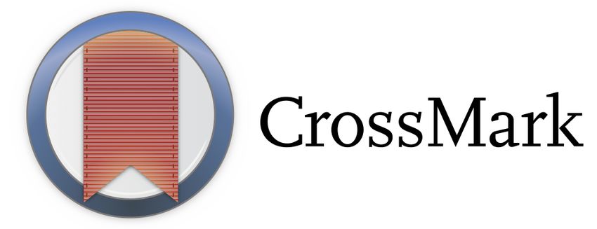
                                                                                                                                                                                                                                              The simulation data with comparison to the universal velocity profile using optimal
                                                                                                                                                                                                                                           parameters for each profile are shown in figure 12(a). The parameters, (k, a, m), lead to
                                                                                                                                                                                                                                           a viscous wall layer that is approximately a third thicker than in channel flow. The outer
                                                                                                                                                                                                                                           flow parameters, (b, n), indicate a smaller outer length scale when compared with channel
                                                                                                                                                                                                                                           flow with a more pronounced wake-like shape, as can be seen in figures 12(a) and 12(b).
                                                                                                                                                                                                                                           The nearly discontinuous decrease in the parameters k and a between Rτ = 2000 and
                                                                                                                                                                                                                                           Rτ = 4000 that occurs in pipe and channel flow is not seen in the boundary layer datasets.
                                                                                                                                                                                                                                           Instead, there is a small increase between the highly resolved LES at Rτ = 2571 and the
                                                                                                                                                                                                                                           experiments at Rτ = 2109 and Rτ = 4374 followed by a decrease in k between Rτ = 4374
                                                                                                                                                                                                                                           and Rτ = 9090.
                                                                                                                                                                                                                                              The largest error between the DNS data and the universal profile is, again, of the
                                                                                                                                                                                                                                           order of 0.1 in units of u+ and occurs in the region 10 < y+ < 20 in the buffer layer.
                                                                                                                                                                                                                                           Nevertheless, the fit for this region is still quite good and, in fact, the universal velocity
                                                                                                                                                                                                                                           profile accurately fits the entire dataset very well. The small variation of the parameters
                                                                                                                                                                                                                                           over all boundary layer datasets supports the applicability of the universal velocity profile,
                                                                                                                                                                                                                                           (3.4) and (3.6), to the boundary layer geometry. Average parameter values from table 1 are
                                                                                                                                                                                                                                           used in figure 12(b) and, again, the optimal and average fits are very close.
                                                                                                                                                                                                                                              The velocity gradient and log indicator function for each boundary layer simulation
                                                                                                                                                                                                                                           case are shown in figure 13. The wake section of the boundary layer profile is much more
                                                                                                                                                                                                                                           933 A16-18
Downloaded from https://www.cambridge.org/core. IP address: 46.4.80.155, on 07 Jan 2022 at 19:03:55, subject to the Cambridge Core terms of use, available at https://www.cambridge.org/core/terms. https://doi.org/10.1017/jfm.2021.998

                                                                                                                                                                                                                                                                        A universal velocity profile for turbulent wall flows
                                                                                                                                                                                                                                             (a) 100                                                  (b) 100

                                                                                                                                                                                                                                                       80                                                       80

                                                                                                                                                                                                                                                       60                                                       60

                                                                                                                                                                                                                                                u+
                                                                                                                                                                                                                                                       40                                                       40

                                                                                                                                                                                                                                                       20                                                       20

                                                                                                                                                                                                                                                        0                                                           0
                                                                                                                                                                                                                                                            100         101              102    103                         100         101          102         103
                                                                                                                                                                                                                                                                                    y+                                                        y+
                                                                                                                                                                                                                                           Figure 12. Turbulent boundary layer DNS data from Simens et al. (2009), Borrell et al. (2013), Sillero et al.
                                                                                                                                                                                                                                           (2013) and Ramis & Schlatter (2014) at Rτ = 1343 (dark blue), 1475 (green), 1616 (dark red), 1779 (yellow),
                                                                                                                                                                                                                                           1962 (purple), 2088 (light blue) and 2571 (light red) compared with the universal velocity profile using (a)
                                                                                                                                                                                                                                           optimal parameters from table 4, (b) average parameters from 1. Profiles are separated vertically by 10 units.

                                                                                                                                                                                                                                            (a) 100                                                     (b) 6

                                                                                                                                                                                                                                                     10–1                                                               5
                                                                                                                                                                                                                                                                  Rτ = 1307
                                                                                                                                                                                                                                                                                                                        4
                                                                                                                                                                                                                                                                                                         y+ (du+/dy+)

                                                                                                                                                                                                                                                                  Rτ = 1437
                                                                                                                                                                                                                                                     10–2
                                                                                                                                                                                                                                           du+/dy+

                                                                                                                                                                                                                                                                  Rτ = 1571
                                                                                                                                                                                                                                                                  Rτ = 1709                                             3
                                                                                                                                                                                                                                                                  Rτ = 1848
                                                                                                                                                                                                                                                     10–3         Rτ = 1989
                                                                                                                                                                                                                                                                  Rτ = 2479
                                                                                                                                                                                                                                                                                                                        2
                                                                                                                                                                                                                                                     10–4
                                                                                                                                                                                                                                                                                                                        1

                                                                                                                                                                                                                                                     10–5                                                               0
                                                                                                                                                                                                                                                                  100         101         102   103                               100         101          102     103
                                                                                                                                                                                                                                                                                y+                                                              y+
                                                                                                                                                                                                                                           Figure 13. Velocity derivative and log indicator function using boundary layer data with average parameters.
                                                                                                                                                                                                                                           The Rτ legend shows values reported with the data for ue /U = 0.99. The Rτ values in table 4 were used to
                                                                                                                                                                                                                                           make the curves. (a) Velocity gradient and (b) log-law indicator function.

                                                                                                                                                                                                                                           pronounced with a larger variation in the gradient compared with channel flow and pipe
                                                                                                                                                                                                                                           flow leading to a substantially larger second peak at ( y+ /δh )III in the wake region of the
                                                                                                                                                                                                                                           log indicator function.

                                                                                                                                                                                                                                                   5.1. The universal profile in the context of the boundary layer equations
                                                                                                                                                                                                                                           The zero pressure gradient form of (1.2a,b) is
                                                                                                                                                                                                                                                                        ∂        ∂       ∂τ   ∂ 2u                           ∂u ∂v
                                                                                                                                                                                                                                                                           (uu) + (uv) =    +ν 2,                               +    = 0.                        (5.1a,b)
                                                                                                                                                                                                                                                                        ∂x       ∂y      ∂y   ∂y                             ∂x   ∂y
                                                                                                                                                                                                                                           The fit of the log indicator function, derived from the universal velocity profile, to the
                                                                                                                                                                                                                                           Ramis & Schlatter (2014) Rτ = 2479 data (Rτ = 2571 in table 4) is shown in figure 14(a).
                                                                                                                                                                                                                                           The fit is at least comparable to and perhaps somewhat better than it was in the channel
                                                                                                                                                                                                                                           flow examples, and the r.m.s. errors presented in table 4 are comparable to or lower than
                                                                                                                                                                                                                                           in the channel flow case. This is a little surprising and raises obvious questions. Why does
                                                                                                                                                                                                                                                                                                                                                            933 A16-19
Downloaded from https://www.cambridge.org/core. IP address: 46.4.80.155, on 07 Jan 2022 at 19:03:55, subject to the Cambridge Core terms of use, available at https://www.cambridge.org/core/terms. https://doi.org/10.1017/jfm.2021.998

                                                                                                                                                                                                                                                                            M.A. Subrahmanyam, B.J. Cantwell and J.J. Alonso
                                                                                                                                                                                                                                             (a) 6                                                                      (b)
                                                                                                                                                                                                                                                                LES data
                                                                                                                                                                                                                                                                Universal profile                                                1.0
                                                                                                                                                                                                                                                            5
                                                                                                                                                                                                                                                                                                                                 0.8
                                                                                                                                                                                                                                             y+ (du+/dy+)

                                                                                                                                                                                                                                                            4

                                                                                                                                                                                                                                                            3                                                           ττ 0.6
                                                                                                                                                                                                                                                            2                                                                    0.4

                                                                                                                                                                                                                                                            1                                                                    0.2

                                                                                                                                                                                                                                                            0                                                                        0
                                                                                                                                                                                                                                                                         100        101       102       103                          10–1          100       101                102       103
                                                                                                                                                                                                                                                                                    y+                                                                            y+
                                                                                                                                                                                                                                           Figure 14. Boundary layer log-law indicator function for Rτ = 2479 Ramis & Schlatter (2014) data
                                                                                                                                                                                                                                           (Rτ = 2571 in table 4) compared with the universal profile and turbulent shear stress data compared with
                                                                                                                                                                                                                                           the shear stress generated using the universal velocity profile in (5.6). The dashed line in panel (b) is the
                                                                                                                                                                                                                                           pipe/channel shear stress generated directly from (3.2) and (3.6). (a) Log indicator function and (b) turbulent
                                                                                                                                                                                                                                           shear stress.

                                                                                                                                                                                                                                           the universal profile derived for pipe flow work so well in the boundary layer and what is
                                                                                                                                                                                                                                           the role of the convective terms in (5.1a,b)?
                                                                                                                                                                                                                                             To examine these questions, we recast (5.1a,b) in wall units. The Kármán integral form
                                                                                                                                                                                                                                           of the boundary layer equation with zero pressure gradient is

                                                                                                                                                                                                                                                                                                                                             2
                                                                                                                                                                                                                                                                                                             dθ   Cf                     uτ
                                                                                                                                                                                                                                                                                                                =    =                             ,                                        (5.2)
                                                                                                                                                                                                                                                                                                             dx   2                      ue

                                                                                                                                                                                                                                           where θ is the boundary layer momentum thickness. The momentum thickness Reynolds
                                                                                                                                                                                                                                           number can be written in terms of wall units as
                                                                                                                                                                                                                                                                                                                                     
                                                                                                                                                                                                                                                                                               ue θ                    Rτ        uτ +
                                                                                                                                                                                                                                                                                          Rθ =      =                       u 1 − u dy+ .
                                                                                                                                                                                                                                                                                                                                +
                                                                                                                                                                                                                                                                                                                                                                                            (5.3)
                                                                                                                                                                                                                                                                                                ν                  0             ue

                                                                                                                                                                                                                                           Equation (5.2) can be rearranged to read

                                                                                                                                                                                                                                                                                                                                
                                                                                                                                                                                                                                                                                                                        uτ 2
                                                                                                                                                                                                                                                                                                                 dRθ     ue
                                                                                                                                                                                                                                                                                                                     =         .                                                            (5.4)
                                                                                                                                                                                                                                                                                                                 dRτ   d (Rτ )
                                                                                                                                                                                                                                                                                                                        dRx

                                                                                                                                                                                                                                           Differentiate (5.3) with respect to Rτ :

                                                                                                                                                                                                                                                                                                                                                               
                                                                                                                                                                                                                                              dRθ    ∂                     Rτ
                                                                                                                                                                                                                                                                                +         +             uτ        ∂             Rτ
                                                                                                                                                                                                                                                                                                                                       +2     +   ∂          uτ            Rτ
                                                                                                                                                                                                                                                                                                                                                                                u+ dy+ . (5.5)
                                                                                                                                                                                                                                                                                                                                                                                      2
                                                                                                                                                                                                                                                  =                             u dy −                                               u      dy −
                                                                                                                                                                                                                                              dRτ   ∂Rτ                0                                ue       ∂Rτ        0                    ∂Rτ         ue        0

                                                                                                                                                                                                                                           Now express (5.1a,b) in wall units and integrate with respect to y+ . Use (5.4) and (5.5)
                                                                                                                                                                                                                                           to replace differentiation in Rx with differentiation in Rτ and solve for the Reynolds stress
                                                                                                                                                                                                                                           933 A16-20
You can also read