What's Up with the Phillips Curve? - Brookings Institution
←
→
Page content transcription
If your browser does not render page correctly, please read the page content below

BPEA Conference Drafts, March 19, 2020

What’s Up with the Phillips Curve?

Marco Del Negro, Federal Reserve Bank of New York
Michele Lenza, European Central Bank
Giorgio E. Primiceri, Northwestern University
Andrea Tambalotti, Federal Reserve Bank of New York

    DO NOT DISTRIBUTE – ALL PAPERS ARE EMBARGOED UNTIL 9:01PM ET 3/18/2020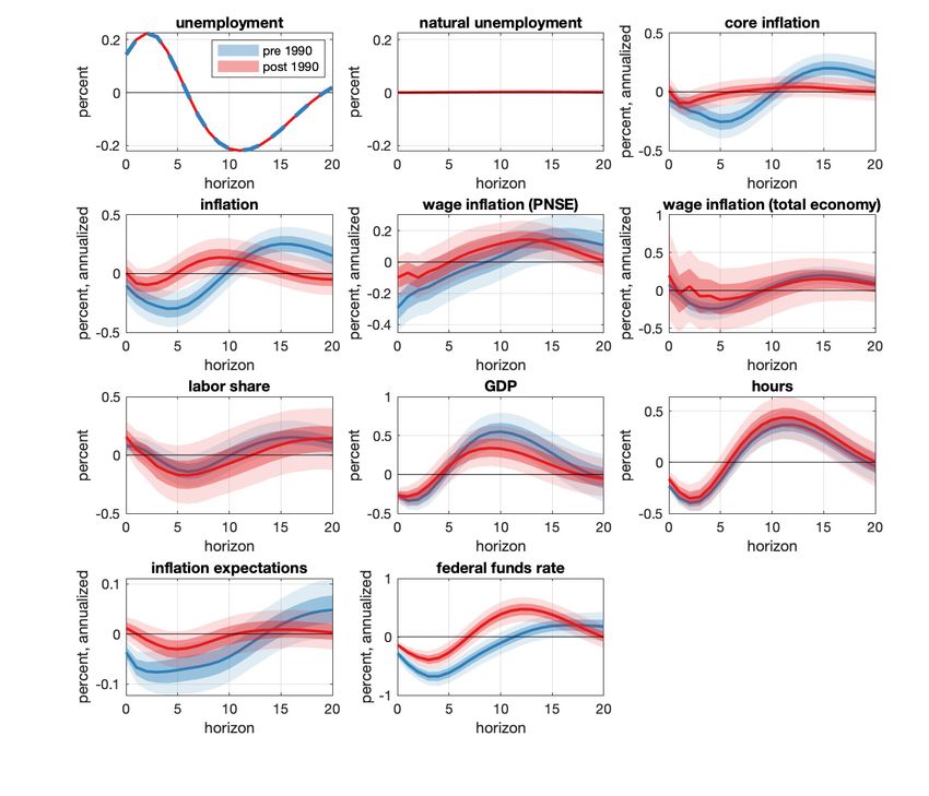
Conflict of Interest Disclosure: Marco Del Negro is Vice President in the Macroeconomic and Monetary Studies
Function of the Research and Statistics Group of the Federal Reserve Bank of New York; Michele Lenza is Head
of Section for the Monetary Policy Research Division of the European Central Bank, the Forecasting and Business
Cycle group leader and research coordinator for the European Central Bank, and a member of the Forecast
Steering Committee for the European Central Bank; Giorgio Primiceri is a professor of economics at
Northwestern University and co-editor of the American Economics Journal; Andrea Tambalotti is Vice President
of the Federal Reserve Bank of New York. Beyond these affiliations, the authors did not receive financial support
from any firm or person for this paper or from any firm or person with a financial or political interest in this
paper. The views expressed in this paper are those of the authors, and do not necessarily reflect those
of Northwestern University, the American Economics Journal, the Federal Reserve Bank of New York, or the
European Central Bank.
WHAT’S UP WITH THE PHILLIPS CURVE?

MARCO DEL NEGRO, MICHELE LENZA, GIORGIO E. PRIMICERI, AND ANDREA TAMBALOTTI

         Abstract. The business cycle is alive and well, and real variables respond to it more
         or less as they always did. Witness the Great Recession. Inflation, in contrast, has gone
         quiescent. This paper studies the sources of this disconnect using VARs and an estimated
         DSGE model. It finds that the disconnect is due primarily to the muted reaction of
         inflation to cost pressures, regardless of how they are measured—a flat aggregate supply
         curve. A shift in policy towards more forceful inflation stabilization also appears to have
         played some role by reducing the impact of demand shocks on the real economy. The
         evidence also rules out stories centered around changes in the structure of the labor
         market or in how we should measure its tightness.

        Key words and phrases: Inflation, unemployment, monetary policy trade-off, VARs,
         DSGE models

                                           1. introduction

   The recent history of inflation and unemployment is a puzzle. The unemployment rate
has gone from below 5 percent in 2006-07 to 10 percent at the end of 2009, and back
down below 4 percent over the past couple of years. These fluctuations are as wide as any
experienced by the U.S. economy in the post-war period. In contrast, inflation has been
as stable as ever, with core inflation almost always between 1 and 2.5 percent, except for
short bouts below 1 percent in the darkest hours of the Great Recession.
   Much has been written about this disconnect between inflation and unemployment. In
the early phase of the expansion, when unemployment was close to 10 percent and inflation
barely dipped below 1 percent, the search was for the “missing deflation” (e.g. Hall, 2011,
Ball and Mazumder, 2011, Coibion and Gorodnichenko, 2015, Del Negro et al., 2015b, Linde

Date: March 2020. PRELIMINARY AND INCOMPLETE. NOT FOR CIRCULATION OR POSTING.
Prepared for the 2020 Spring Brookings Papers on Economic Activity. We thank Ethan Matlin and espe-
cially William Chen for excellent research assistance, and Olivier Blanchard, Keshav Dogra, Simon Gilchrist,
Pierre-Olivier Gourinchas, and Argia Sbordone for useful comments and suggestions. Jim Stock provided
much appreciated guidance during the research and writing process. The views expressed in this paper are
those of the authors and do not necessarily represent those of the European Central Bank, the Eurosystem,
the Federal Reserve Bank of New York, or the Federal Reserve System.
                                                     1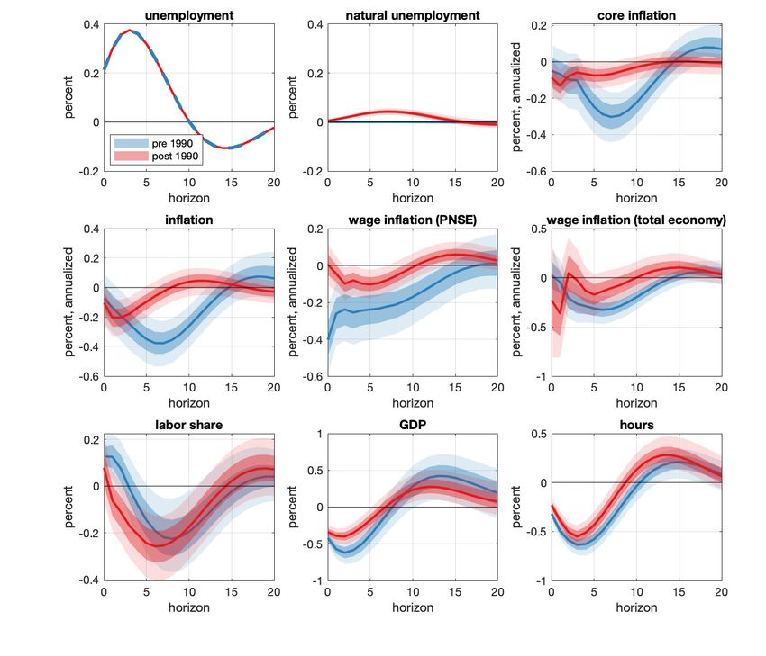
WHAT’S UP WITH THE PHILLIPS CURVE?                                  2

and Trabandt, 2019). More recently, with unemployment below 5 percent for almost four
years and inflation persistently under 2 percent, attention has turned to factors that might
explain why inflation is not coming back (e.g. Powell, 2019, Yellen, 2019). Beyond this
recent episode, a reduction in the cyclical correlation between inflation and real activity
has been evident at least since the 1990s (e.g. Atkeson and Ohanian, 2001, Stock and
Watson, 2008, Stock and Watson, 2007, Zhang et al., 2018 and Stock and Watson, 2019).
The literature, which we review in more detail below, has focused on four main classes of
explanations for this puzzle: (i) mis-measurement of either inflation or economic slack; (ii)
a flatter wage Phillips curve; (iii) a flatter price Phillips curve; and (iv) a flatter aggre-
gate demand relationship, induced by an improvement in the ability of policy to stabilize
inflation.
  This paper tries to distinguish among these four competing hypotheses using a variety
of time-series methods. We find overwhelming evidence in favor of a flatter price Phillips
curve. Some of the evidence is also consistent with a change in policy that has led to a
flatter aggregate demand relationship.
  The analysis starts by illustrating a set of empirical facts regarding the dynamics of in-
flation in relation to other macroeconomic variables, using a vector autoregression (VAR).
Many of these facts are already known, but the dynamic, multivariate perspective offered
by the VAR makes it easier to consider them jointly, enhancing our ability to point towards
promising explanations for the phenomenon of interest. First, goods inflation has become
much less sensitive to the business cycle after 1990, consistent with most of the literature
on the severe illness of the Phillips curve. Second, this is true to a much lesser extent for
wage inflation: the wage Phillips curve is in better health than that of good inflation, as
also found by Coibion et al. (2013), Coibion and Gorodnichenko (2015), Gali and Gambetti
(2018), Hooper et al. (2019) and Rognlie (2019). Third, there is little change before and
after 1990 in the business cycle dynamics of the most popular indicators of inflationary
pressures relative to each other, especially when compared to the pronounced reduction in
the responsiveness of inflation. These indicators include measures of labor market activ-
ity, such as the unemployment rate and its deviations from the natural rate, hours, the
employment-to-population ratio and unit labor costs, as well as broader notions of resource
utilization, such as GDP and its deviation from measures of potential. Fourth, the decline
in the sensitivity of inflation to the business cycle is heterogenous across goods and services.
WHAT’S UP WITH THE PHILLIPS CURVE?                                           3

In particular, Stock and Watson (2019) document that the relationship between cyclical
unemployment and inflation has changed very little over time for certain categories of goods
and services that are better measured and less exposed to international competition. Our
VAR analysis produces results that are consistent with these findings, but we do not report
them here since they are not necessary to draw our main conclusions.1
    Together, the first three empirical facts listed above lead us to reject the mis-measurement
of economic slack, as well as a significant flattening of the wage Phillips curve, as the main
drivers of the inflation-real activity disconnect. The evidence sustaining this conclusion is
that the relationship between the most common indicators of cost pressures has not changed
much before and after 1990, while at the same time inflation became way more stable.2 A
further implication of this finding is that we can focus the rest of the investigation on the bi-
variate relationship between inflation and real activity, without having to take a stance on
the most appropriate measure of the latter. Any indicator commonly used in the literature
will do.3
    This conclusion marks the boundary to which we can push the VAR for purely descrip-
tive purposes. As illustrated in a recent influential paper by McLeay and Tenreyro (2019),
the observed relationship between inflation and real activity is the result of the interaction
between aggregate demand and supply. The latter captures the positive relationship be-
tween inflation and real activity, usually associated with the price Phillips curve. Higher
inflation is connected with higher marginal costs, which in turn tend to rise in expansions
when demand is high, the labor market is tight, and wages are under pressure. On the con-
trary, the economy’s aggregate demand captures a negative relationship between inflation
and real activity, which reflects the endogenous response of monetary policy to inflationary

1
 Some recent papers have also explored the behavior of inflation across geographic areas in the United States
and across countries (e.g. Fitzgerald and Nicolini, 2014, Mavroeidis et al. 2014, McLeay and Tenreyro 2019,
Hooper et al. 2019, and Geerolf, 2019). They generally find that the correlation between inflation and
unemployment in the cross-section is stronger and more stable than in the time-series. Hazell et al. (2020)
provide a guide to translate those cross-sectional correlations in terms of the time-series correlation that is
of interest to most of the macroeconomics literature. Using data on U.S. states, they recover a flat Phillips
curve once the estimates are properly re-scaled, with a further reduction in the slope coefficient after 1985.
2
 We cannot rule out that all the indicators of cost pressures that we include in our analysis have become a
poorer proxy for the “true” real marginal costs that drive firms’ pricing decisions after 1990. However, it is
unlikely that an unobserved change in the dynamics of those costs could have left almost no trace on the
joint dynamics of all those indicators.
3
 In practice, we focus primarily on the relationship between inflation and unemployment, but continue to do
so in the context of a VAR that also includes other macroeconomic variables. We focus on unemployment
because the latter is arguably the most straightforward and widely-discussed measure of the health of the
real economy, as well as the most commonly used independent variable in Phillips curve regressions.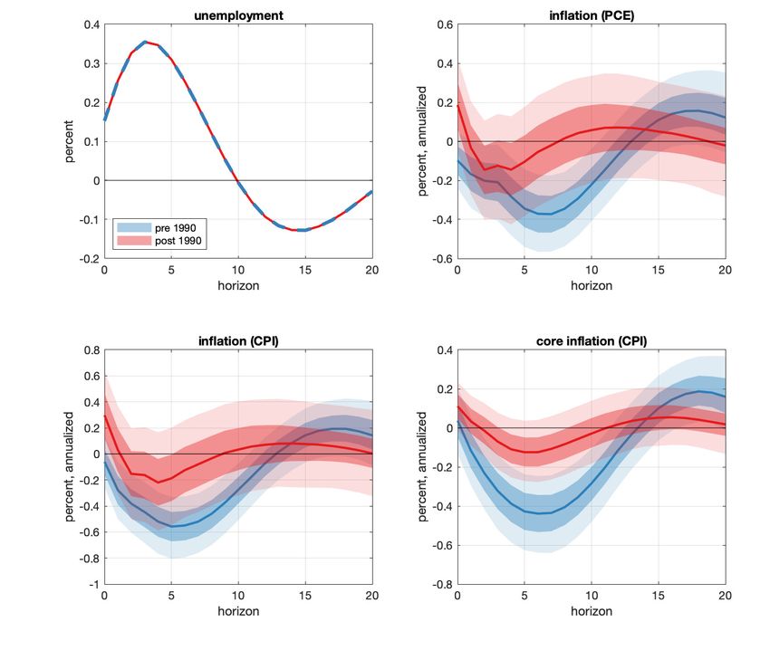
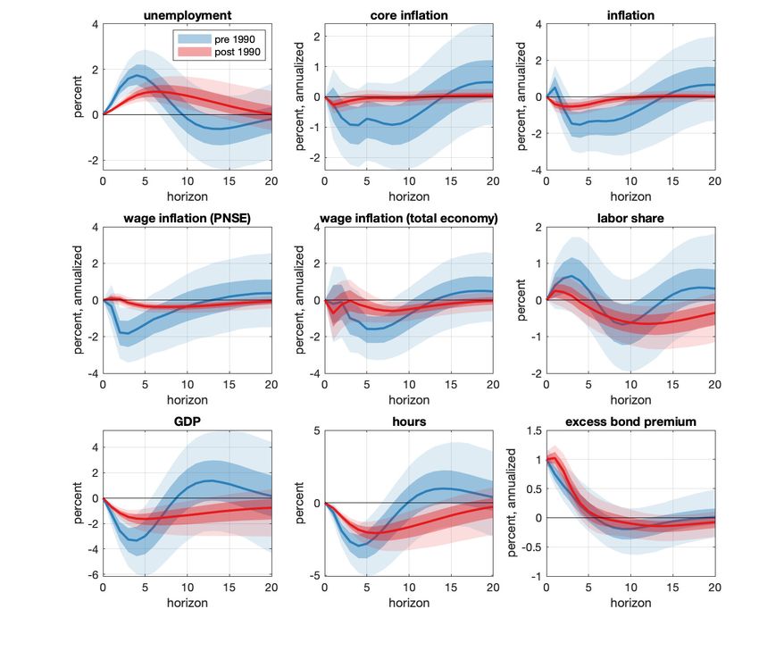
WHAT’S UP WITH THE PHILLIPS CURVE?                                4

pressures. When inflation is high, the central bank tightens monetary policy, thus slowing
the real economy. Therefore, the observed cyclical disconnect between inflation and real
activity might be the result of either a flat Phillips curve—the slope hypothesis—or a flat
aggregate demand, generated by a forceful response of monetary policy to inflation. In the
limit in which the central bank pursues perfect inflation stability, inflation is observed to
be insensitive to the cycle, regardless of the slope of the Phillips curve. We refer to this
second possible explanation for the stability of inflation as the policy hypothesis.
  Distinguishing between these two hypotheses is a classic identification problem that re-
quires economic assumptions that were not needed for the data description exercise in
the first part of the paper. We impose those restrictions through two complementary
approaches, a structural VAR (SVAR) and an estimated dynamic stochastic general equi-
librium (DSGE) model. In the SVAR, we identify cyclical fluctuations that can be plausibly
attributed to a demand disturbance. To do so, we follow Gilchrist and Zakrajsek (2012) and
use their data on the excess bond premium (EBP) to identify a financial shock that prop-
agates through the economy like a typical demand shock, by depressing both real activity
and inflation. We choose this shock as a proxy for demand disturbances because it accounts
for a significant fraction of the business cycle fluctuations behind the facts described in the
first part of the paper. In response to this demand shock, inflation barely reacts in the post-
1990 sample, while it used to fall significantly before. This result indicates that the slope
of the aggregate supply relationship must have fallen since 1990. Intuitively, the demand
shock acts as an instrument for cost pressures in the Phillips curve, identifying its slope. If
real activity declines in response to an EBP shock, as it clearly does in both samples, and
this lowers cost pressures (i.e. if the instrument is not weak), a muted response of inflation
implies a flat Phillips curve.
  Although this evidence clearly points in the direction of a very flat aggregate supply
curve after 1990, it does not rule out the possibility that monetary policy might have also
contributed to the observed stability of inflation. In fact, the main implication of this
hypothesis is that monetary policy should lean more heavily against inflation by limiting
the impact of demand shocks on the real fluctuations. In the limit in which inflation
is perfectly stable, demand shocks should leave no footprint on the real variables. The
impulse responses to the EBP shock are far from implying no reaction of the real variables
WHAT’S UP WITH THE PHILLIPS CURVE?                                   5

to the demand disturbance, as we would expect if the stability of inflation were due to
monetary policy, although they do point to some stabilization, at least in the short run.
  The SVAR evidence that we just described still leaves (at least) two explanations for the
stability of inflation on the table, even if it helps to narrow down their relative contributions.
In this respect, our interpretation is that the evidence leaves little doubt that the slope of
the Phillips curve is currently very low, but it is also consistent with a contribution to the
overall stability of inflation from a flatter aggregate demand curve. To provide a sharper
quantification of the relative roles of these two changes, we turn to an estimated DSGE
model. This exercise is subject to the typical trade-off associated with imposing tighter
economic restrictions on the data. On the one hand, we can map the slope and policy
hypotheses directly into parameters of the model that we can estimate on data before and
after 1990. On the other hand, the results of this exercise hinge on the entire structure of
the model, rather than on a looser set of identifying assumptions as in the SVAR. Therefore,
they stand or fall together with the observer’s believes on the validity of that structure as
a representation of the data. To support the case in favor of the model’s validity for our
purposes, we show that it reproduces the facts generated by the reduced-form VAR used for
data description in the first part of the paper. In terms of the two hypotheses, the DSGE
estimates point in the direction of a much flatter Phillips curve in the second sample. If we
assume that the slope of the Phillips curve is the only parameter that changes after 1990,
the estimated model still broadly reproduces the empirical facts. If we only allow policy to
change, the estimated model falls short.
  Together, the results of the SVAR and DSGE produce two more conclusions. First, the
slope hypothesis is correct: the slope of the Phillips curve is extremely low after 1990,
although it is not zero. Second, there is less clear-cut evidence in favor of the policy
hypothesis. Changes in the conduct of policy, or other structural changes contributing to a
flatter aggregate demand curve, also appear partly responsible for the reduced sensitivity
of inflation to cyclical impulses.
  The rest of the paper proceeds as follows. The remainder of this section reviews the
literature. Section 2 describes the VAR that we use for data description, whose results are
then described in section 3. Section 4 introduces a stylized aggregate demand and supply
framework inspired by McLeay and Tenreyro (2019), which illustrates the fundamental
identification problem underlying the interpretation of the observed relationship between
WHAT’S UP WITH THE PHILLIPS CURVE?                                           6

inflation and real activity. This model also guides the interpretation of the impulse responses
to the EBP shock presented in section 5. Section 6 revisits the same facts presented in
section 3 from the perspective of an estimated DSGE model, and uses that model to further
explore the relative contribution of the slope and policy hypothesis to the observed stability
of inflation. Section 7 elaborates on some policy implications of our main findings, before
offering some concluding remarks in section 8.

The literature. The literature has explored four main classes of explanations for the
reduction in the observed correlation between inflation and real activity.
    The first set of explanations is related to mis-measurement of either inflation or economic
slack. In the inflation dimension, much of the debate has focused on the role of new products
and quality adjustment in the construction of price indexes and in the measurement of
output and productivity, especially following the introduction of technologies with a very
visible impact on everyday life, such as the internet and smart phones (e.g. Moulton, 2018).
This branch of the literature has also explored the recent emergence of online retailing
as a source of transformation in firms’ pricing practices (e.g. Cavallo, 2018, Goolsbee
and Klenow, 2018). By focusing on cyclical fluctuations, our analysis mostly bypasses
these considerations, since they primarily pertain to the level of measured inflation. In
addition, the inflation-real activity disconnect predates the potential effect of information
technology on price mis-measurement, further reducing the potential explanatory power of
this hypothesis for our phenomenon of interest.
    On the real activity front, a long-standing issue is how to measure economic slack and
the amount of inflationary pressures emanating from it.4 In this respect, our results on the
stability of the co-movement of various measures of cost pressures should reduce the weight
put on explanations of the inflation disconnect based on the idea that any measure of slack
might be less representative of underlying inflationary pressures after 1990, for instance due
to changes in the relationship between measured unemployment and the overall health of
the labor market (e.g. Stock, 2011, Gordon, 2013, Hong et al., 2018, Ball and Mazumder,
2019).

4
 A large body of work focuses on the estimation of potential output and the natural rate of unemployment
as reference points to assess the cyclical position of the economy (e.g. Abraham et al., 2020 in this volume).
Crump et al., 2019 provide a comprehensive discussion of the literature on the natural rate of unemployment
and its definition and measurement, which features many prominent contributions in the Brookings papers.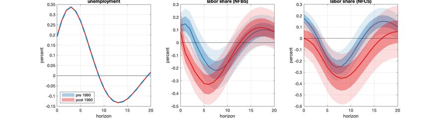
WHAT’S UP WITH THE PHILLIPS CURVE?                                   7

  A second set of explanations, which in some cases connect with the mis-measurement
of slack we just discussed, focuses on a flatter wage Phillips curve and more in general
on structural transformations of the labor market and/or of its connection with the goods
market (e.g. Daly and Hobijn, 2014, Stansbury and Summers, 2020, Faccini and Melosi,
2020). While the structure of the labor market surely underwent major changes over the
past decades, our results suggest that these transformations may not be the leading cause
of inflation stability.
  A third set of explanations focuses on the role of policy in delivering stable inflation.
The idea is that a stronger response of monetary policy to inflation flattens the aggregate
demand curve, weakening the connection between inflation and real fluctuations, even if the
aggregate supply relationship is unchanged (e.g. Fitzgerald and Nicolini, 2014, Barnichon
and Mesters, 2019a, and McLeay and Tenreyro, 2019, echoing older work by Kareken and
Solow, 1963 and Goldfeld and Blinder, 1972). We also find that monetary policy probably
played some role in stabilizing inflation over the cycle. However, our evidence suggests that
policy did not entirely succeed in eliminating demand-driven real fluctuations, implying
that it cannot be the dominant driver of the inflation-real activity disconnect. This result,
however, does not imply that changes in monetary (and perhaps fiscal) policy were not a
major source of the low frequency fluctuations in inflation related to its slow rise between
the mid 1960s and 1979 and its return to 2 percent over the subsequent two decades, as
argued, for instance, by Primiceri (2006).
  Related to this policy hypothesis is the large literature on the role of inflation expectations
and their anchoring (e.g. Orphanides and Williams, 2005, Bernanke, 2007, Stock, 2011,
Blanchard et al., 2015, Blanchard, 2016, Ball and Mazumder, 2019, Carvalho et al., 2019,
Jorgensen and Lansing, 2019, and Barnichon and Mesters, 2019c). Empirically, expectations
are now less volatile than they were before 1990, as we also find in our VAR. However,
this observation does not establish that changes in their formation, perhaps in response
to shifts in the conduct or communication of policy, represent an autonomous source of
inflation stability. Rather, our evidence suggests that the behavior of inflation expectations
mostly reflects the inflation stability induced by the flattening of the aggregate supply curve,
instead of being its primary source.
  In conclusion, our results support a fourth set of explanations that attribute the inflation-
real activity disconnect to forces that dull the response of goods prices to the cost pressures
WHAT’S UP WITH THE PHILLIPS CURVE?                                       8

faced by firms, lowering the slope of the “structural” price Phillips curve. This is the slope
hypothesis, which takes several variants. The most prominent is the one that attributes a
reduction in the response of prices to marginal costs to the increased relevance of global
supply chains, heightened international competition, and other effects of globalization (e.g.
Sbordone, 2007, Auer and Fischer, 2010, Rich et al., 2013, Tallman and Zaman, 2017,
Forbes, 2019a, Forbes, 2019b, and Obstfeld, 2019). In a similar vein, Rubbo (2020) points
to changes in the network structure of the U.S. production sector.5

                                  2. Methodology and Data

    The objective of this paper is to shed light on the possible causes of the widely acknowl-
edged attenuation of the response of inflation to labor market slack over the past three
decades. This section illustrates the methodology and the data that we use to document
this fact, and its relationship with the behavior of a broad set of macroeconomic variables,
whose joint dynamics might help to discriminate among alternative explanations.

2.1. Methodology. To study macroeconomic dynamics and their change over time, we
begin by adopting the following Vector-Autoregression (VAR) model:

(2.1)                          yt = c + B 1 y t   1   + ... + Bp yt   p   + ut .

In this expression, yt is an n ⇥ 1 vector of macroeconomic variables, which is modeled as
a function of its own past values, a constant term, and an n ⇥ 1 vector of forecast errors
(ut ) with covariance matrix ⌃. The reduced-form shocks (ut ) are a linear combinations of
n orthogonal structural disturbances ("t ), which we write as ut = "t .
    VARs are flexible multivariate time-series models, which provide a rich account of the
complex forms of autocorrelation and cross-correlation that are typical of macroeconomic
variables. To synthesize and illustrate these relationships, we study the dynamic response of
the variables of interest to a typical business cycle (BC) shock. We define this shock as the
linear combination of structural disturbances that drives the largest share of unemployment

5
 Afrouzi and Yang (2019) connect changes in the conduct of monetary policy directly to the slope of the
Phillips curve, straddling the two strands of the literature that we just discussed. They present a model
in which rationally inattentive price setters respond less to aggregate shocks when monetary policy is
committed to inflation stabilization.
WHAT’S UP WITH THE PHILLIPS CURVE? 9
variation at business cycle frequencies, as in Giannone et al. (2019) and Angeletos et al.
(2019).6
This approach does not attempt to pin down the precise identity of the structural dis-
turbances driving fluctuations, as in more typical structural VARs. Doing so would require
additional economic assumptions, which are not necessary to document many of the em-
pirical facts regarding the attenuated response of inflation to labor market slack that have
been discussed in the literature. The advantage of this methodology is that we can illustrate
these facts in the context of a unified, dynamic, multivariate statistical framework, without
imposing any theoretical restriction. Its obvious disadvantage is that, without economic
restrictions, those facts can be mapped into more than one hypothesis on the sources of the
increased disconnect between inflation and real activity. Therefore, section 5 and 6 will also
explore more economically-demanding approaches—SVARs and DSGE models—in order to
further pinpoint the source of the empirical observations illustrated below.
The VAR approach to data description that we pursue in this section has also some
advantages over the much more popular direct estimation of a Phillips curve, defined as the
relationship between inflation (and its lags) and some measure of slack. First, such an in-
flation equation is embedded in the VAR, which therefore encompasses the single-equation
approaches as long as the same variables used in them are included in yt . Second, embed-
ding such an equation into a multivariate framework explicitly recognizes the challenging
identification problem of distinguishing a Phillips curve, which represents the economy’s
aggregate supply, from its aggregate demand. We illustrate this challenge in the context of
a stylized New Keynesian model in section 4. Third, looking at the response of inflation and
the other variables to the combination of shocks responsible for the bulk of business cycle
fluctuations produces more flexible measures of economic slack than those based on specific
indicators of potential output or natural unemployment—two notoriously elusive concepts.
Fourth, we do not need explicit measures, or a model, of inflation expectations, as long as
the variables included in the VAR approximately span the information set used by agents
6More precisely, we compute the spectral density of y implied by the VAR representation (2.1). We use this
t
spectrum to evaluate the variance of unemployment at business cycle frequencies (those related to periods
of length between 6 and 32 quarters, as in Stock and Watson, 1999), as a function of the columns of all
1
possible ⌃ 2 matrices. The BC shock is pinned down by the column associated with the maximal variance
of unemployment at these frequencies. For technical details and the specific implementation of this idea,
see Giannone et al. (2019) and Angeletos et al. (2019).WHAT’S UP WITH THE PHILLIPS CURVE? 10 to form those expectations. This aspect of the analysis is especially important, since infla- tion expectations are a key ingredient in most formulations of the Phillips curve. For this reason, we also consider VAR specifications that include a direct measure of expectations in the vector yt . 2.2. Data. What variables should the VAR include to provide a comprehensive view of the forces shaping the connection between inflation and the labor market? To answer this question, we refer to an intuitive description of that connection, which is embedded in most formal and informal frameworks built around a price and/or wage Phillips curve.7 When firms try to hire more workers to satisfy higher demand for their output, wages tend to rise. Given labor productivity, this increase in wages is associated with higher marginal costs and inflation. Therefore, a tight labor market, rising wages, costs and inflation tend to occur together in response to demand shocks. To characterize these channels, data on inflation and unemployment are not enough. In addition, we need measures of wages, labor productivity, and firms’ costs to help capture the intermediate steps of the transmission. Therefore, we propose a baseline VAR that includes 8 macroeconomic variables: (i) unemployment, measured by the civilian unemployment rate; (ii) natural unemployment, measured by the CBO estimate; (iii) core inflation, mea- sured by the annualized quarterly growth rate of the Personal Consumption Expenditures price index, excluding food and energy; (iv) inflation, measured by the annualized quarterly growth rate of the GDP deflator; (v) GDP, measured by the logarithm of per-capita real GDP; (vi) hours, measured by the logarithm of per-capita hours worked in the total econ- omy; (vii) wage inflation, measured by the annualized quarterly growth rate of the average hourly earnings of production and nonsupervisory employees (PNSE); and (viii) the labor share, measured by the logarithm of the share of labor compensation in GDP. Appendix A describes the data, their sources and transformations in more detail. Besides unemployment, this VAR includes a block of variables referring to the total economy: GDP, hours, the labor share, and the GDP deflator. These variables can be combined to compute a measure of hourly nominal compensation in the total economy. The growth rate of this measure of nominal wages closely tracks compensation per hour in the nonfarm business sector, a commonly used indicator of labor costs. The problem with both 7A simple example of such a framework is the New-Keynesian model with sticky wages and prices in Chapter 6 of Galí (2015).
WHAT’S UP WITH THE PHILLIPS CURVE? 11
these series is that they are extremely volatile at high frequencies, obscuring the underlying
wage dynamics over the business cycle. For this reason, the baseline VAR also includes the
PNSE wage inflation series. This series only covers 80 percent of private industries, but it
is substantially less noisy than the more comprehensive ones that we mentioned. Finally, in
addition to GDP inflation, our model also includes core PCE inflation, given its importance
as a gauge of underlying inflationary pressures.
We estimate this 8-variable VAR over two non-overlapping samples, to investigate pos-
sible changes in the typical co-movement pattern of these variables in response to the BC
shock described in section 2.1. The first sample ranges from 1964:II to 1989:IV, and the
second from 1989:I to 2019:III.8 The analysis starts in 1964:II because that is when the
PNSE wage inflation series becomes available. The date at which we split the sample is
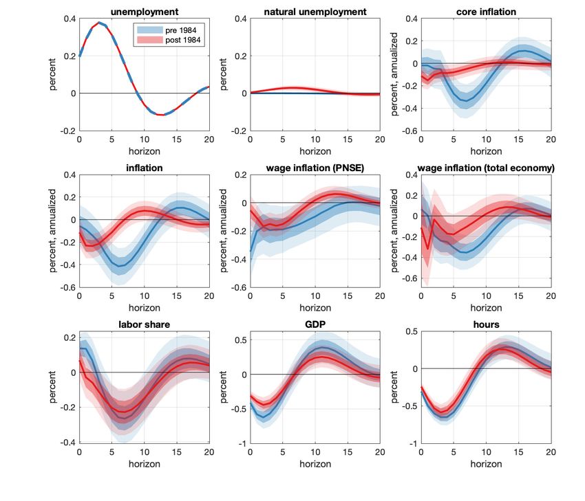
the result of a compromise. On the one hand, there is some evidence that macroeconomic
dynamics might have changed around 1984, after the first phase of the so-called Volcker
disinflation. On the other hand, a simple inspection of the data suggests that inflation
has been most stable starting around the mid 1990s, after the opportunistic disinflation
engineered by the Federal Reserve under Alan Greenspan following the 1990-91 recession.
As a compromise between these two alternatives, we split the sample in 1990. This choice
also has the advantage of creating two samples of fairly similar lengths. Section B shows
that this choice is immaterial for the results.
The data are quarterly and the VAR includes 4 lags. It is estimated with Bayesian
methods and a standard Minnesota prior, given the relatively high number of variables and
short sample sizes. The tightness of the prior is chosen based on the data-driven method
described in Giannone et al. (2015).
3. Facts
This section documents a number of known and new facts concerning the relationship
between unemployment, inflation, and some other key macroeconomic variables. These em-
pirical findings lead us to two main conclusions: (i) the attenuation of inflation fluctuations
over the business cycle before and after 1990 is striking; (ii) in comparison, the co-movement
of all real variables and indicators of firms’ cost pressures has been remarkably stable.
8The first four observations are used as initial conditions, since our VAR has four lags. Therefore, effectively,
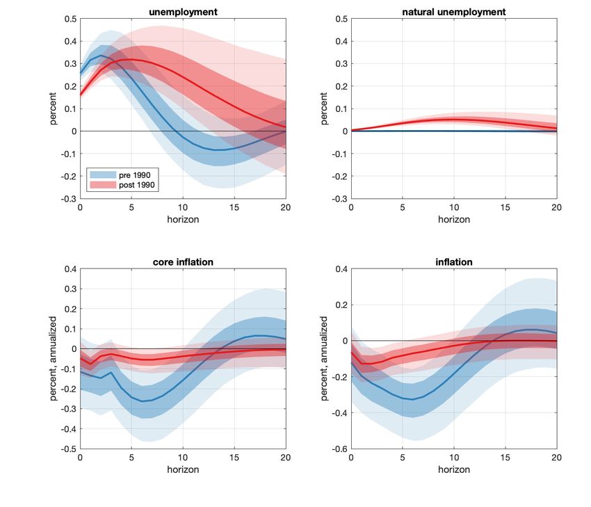
the estimation starts in 1965:II in the first sample and in 1990:I in the second one.WHAT’S UP WITH THE PHILLIPS CURVE? 12 3.1. Fact 1: Unemployment and price inflation. We begin by presenting the impulse responses of unemployment and inflation to a BC shock in the two samples. Figure 3.1 shows that inflation falls significantly as unemployment rises in the first sample. This finding suggests that the BC shock is characterized by a strong demand component, which explains why traditional Phillips curves estimated over this sample have a negative slope. In the second sample, instead, unemployment increases by a roughly similar amount, but the responses of both inflation measures are muted. In fact, the response of core inflation is statistically indistinguishable from zero throughout the horizon, while that of GDP inflation is a bit more negative and borderline significant after about one year. In addition, the very flat response of natural unemployment confirms that the shock only captures business cycle variation. Therefore, looking at the reaction of unemployment or the unemployment gap to this shock would produce identical results.9 The response of unemployment to a BC shock in figure 3.1 is more persistent in the second sample. This feature of economic fluctuations is evident even from the raw data, and it is consistent with the lengthening of expansions in the last thirty years. However, this change in the profile of unemployment fluctuations does not play much of a role in accounting for the attenuated response of inflation in the second sample. We illustrate this point with an exercise that forces the response of unemployment to be identical in the two samples. Specifically, we adopt the conditional-forecast methodology of Banbura et al. (2015) to compute the behavior of all the VAR variables, conditional on unemployment following the same path in both samples. As this common path, we choose the median response of unemployment to a BC shock in the first sample.10 Figure 3.2 plots the dynamics of all the VAR variables in this conditional forecast exercise. As in figure 3.1, the response of inflation in the second sample is much attenuated, although it now remains negative. Appendix B shows that this change in inflation dynamics over the two samples is not limited to the two measures of inflation included in the baseline VAR, but it extends to a number of other commonly used inflation series. 9Appendix B shows that the responses of figure 3.1 are nearly identical to those to an unemployment shock using a Cholesky identification with unemployment ordered first. This result suggests that the combination of shocks responsible for the bulk of business cycle fluctuations and the one associated with the one-step- ahead forecast error in unemployment are virtually the same. 10This conditional forecast approach recovers the most likely sequence of shocks to guarantee that un- employment follows a given path. In this respect, it has a slightly different interpretation relative to the impulse responses, because the latter are based on a single shock perturbing the economy at horizon zero.
WHAT’S UP WITH THE PHILLIPS CURVE?                                    13

         Figure 3.1. Impulse responses of unemployment and price inflation to a business cycle
         shock. The impulse responses are from the baseline VAR described in section 2.2. The
         BC shock is identified with the methodology discussed in section 2.1. The solid lines
         are posterior medians, while the shaded areas correspond to 68- and 95-percent posterior
         credible regions. The pre- and post-1990 samples consist of data from 1964:II to 1989:IV,
         and from 1989:I to 2019:III, respectively.

  These findings can be summarized into a first key stylized fact: The sensitivity of goods
price inflation to labor market slack has decreased dramatically after 1990. This fact pro-
vides a complementary, more dynamic, characterization of many findings in the literature
regarding the stability of inflation. Interpreting this fact is the main task of the rest of the
paper.

3.2. Fact 2: Unemployment and wage inflation. A substantial body of recent work
finds that the connection of wage inflation to labor market slack remains stronger than
WHAT’S UP WITH THE PHILLIPS CURVE? 14
Figure 3.2. Forecasts of all variables, conditional on unemployment following the
path in the first subplot. The conditional forecasts are from the baseline VAR described
in section 2.2. The solid lines are posterior medians, while the shaded areas correspond
to 68- and 95-percent posterior credible regions. The pre- and post-1990 samples consist
of data from 1964:II to 1989:IV, and from 1989:I to 2019:III, respectively.
that of goods inflation (Gali and Gambetti, 2018, Hooper et al., 2019, Rognlie, 2019). This
section presents VAR results broadly consistent with these findings. The second row of
figure 3.2 plots the response of two measures of nominal wage inflation using the conditional
forecast approach described in the previous subsection. The first measure (PNSE) is the
one used directly for the estimation of the baseline VAR. The second (total economy) is
that implied by the data on the labor share, hours, output and GDP inflation.11 The
11In logs, the labor share (ls) is defined as the sum of the nominal wage (w) and hours (h), minus real
GDP (gdp) and the price level (p), or ls ⌘ w + h gdp p. Therefore, this measure of the (log) nominal
wage is constructed as w = ls h + gdp + p.WHAT’S UP WITH THE PHILLIPS CURVE? 15
reaction of the PNSE series is attenuated in the post-1990 period, while the response of
the total-economy measure shows more similarities in the two samples. Therefore, we take
the balance of the evidence as consistent with the view that the connection between wage
inflation and unemployment remains alive, although it is weaker in the more recent period.
As shown in appendix B, the sensitivity of wage inflation to unemployment after 1990 is
even stronger when wages are measured with the employment cost index (ECI), which is
arguably a better measure of the cyclicality of wages than the ones used in this section.
Unfortunately, the ECI is only available starting in 1980, preventing a full comparison of its
behavior pre and post 1990. We summarize these findings in the form of a second stylized
fact: The sensitivity of nominal wage inflation to labor market slack has diminished after
1990, but less than that of price inflation.
One implication of this fact is that explanations of the unemployment-inflation disconnect
involving a much reduced responsiveness of wage inflation to labor market slack are not
very plausible. For example, a popular narrative attributes the stability of inflation during
the Great Recession to the existence of downward nominal wage rigidities: If firms are
reluctant or unable to lower nominal wages, their marginal costs should remain relatively
high, putting upward pressure on prices and inflation. Such a story, however, would imply
a substantial weakening of the comovement between unemployment and wage inflation,
which seems at odds with the data. In addition, as we demonstrate in appendix B, this
co-movement is approximately equally strong in the post-1990 period, regardless of whether
we include or exclude the Great Recession period.
3.3. Fact 3: Unemployment and unit labor costs. One obvious difficulty in inter-
preting the evidence on the connection between nominal wage inflation and unemployment
presented in the previous section is that it also partly reflects a weaker response of goods
inflation. Mechanically, nominal wage inflation is the sum of real wage inflation and goods
inflation. Therefore, the former will appear less responsive to the cycle if the latter is,
given the dynamics of the real wage. A more helpful approach to evaluate the implications
of wage dynamics for inflation, therefore, is to study more direct measures of how wages
contribute to firms’ marginal costs.12 The most popular proxy for aggregate real marginal
costs are unit labor costs, (or, equivalently, the labor share). With constant returns in
12
In pricing problems based on cost minimization, firms’ marginal costs are the key driver of their pricing
decisions. As a result, the evolution of aggregate marginal costs is the fundamental source of inflation in
a large class of models with nominal rigidities. These models include those with staggered price setting,WHAT’S UP WITH THE PHILLIPS CURVE? 16 production, (log) unit labor costs are proportional to (log) marginal costs. Under more general assumptions, this proportionality no longer holds, but unit labor costs are likely to remain a more accurate gauge of the cost pressures faced by firms than nominal wage inflation.13 Figure 3.2 shows that the forecast of the labor share conditional on the usual path of unemployment is very similar in the two samples. This observation leads to the third stylized fact: The co-movement of unemployment and the labor share over the business cycle is stable over time. This fact supports and further refines the view according to which labor market developments are unlikely to be the main source of the change in inflation dynamics over the past thirty years. The claim is not that labor market dynamics have not changed since 1990. More narrowly, the statement is that, whatever those changes might have been, they did not have a significant impact on the dynamics of firms’ marginal costs, at least as seen through the lens of a proxy such as the labor share. The next section adds one further dimension to this claim, by showing that the same can be said of other well known aggregate proxies for firms’ cost pressures. 3.4. Fact 4: Unemployment and other measures of real activity. The previous subsection argued that unit labor costs are likely to be the most informative variable on the extent to which cost pressures originating in the labor market are transmitted to goods prices.14 Next, we show that the dynamics of many other variables used in the literature to capture real sources of inflationary pressure, from the labor market or otherwise, are also relatively stable over time. The third row of figure 3.2 reports the conditional forecasts of hours and output. These responses are essentially identical over time, implying a fourth stylized fact: the business cycle correlation among several indicators of real activity has not changed in the two samples. Appendix B further shows that these empirical patterns as in Calvo (1983) and Taylor (1980), as well as those with sticky information or rational inattention, as inMankiw and Reis (2002) or Mackowiak and Wiederholt (2009). 13 With constant returns to scale production, a firm’s log marginal cost is proportional to its log unit labor cost, defined as ulc = w (gdp h). With homogeneous factor markets, marginal cost is equalized across firms, so that the aggregate log labor share (ls = w + h gdp p) is proportional to the average real marginal cost. 14 A key implication of firms’ cost minimization is that marginal cost is equalized across all inputs. As a result, marginal cost pressures—measured by comparing wages to labor productivity—provide a com- prehensive view of the cost pressures faced by firms, even if the input whose direct cost is rising is not labor. The main difficulty in operationalizing this observation is the measurement of the marginal cost and marginal benefit of labor, i.e. the “wage” and the marginal product of labor. Available measures of wages and (average) labor productivity capture those marginal concepts only under restrictive assumptions.
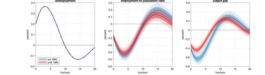
WHAT’S UP WITH THE PHILLIPS CURVE?                              17

also hold for the output gap and the employment-to-population ratio, when we add these
variables to the baseline VAR.
     The important conclusion that we draw from these results is that the severe illness of the
reduced-form relationship between inflation and real activity cannot be cured by picking a
different indicator of either labor or goods market slack among those commonly used in the
literature. In fact, the remarkable stability in the dynamic relationships between all the real
variables that we have considered suggests that the diagnosis of what ails inflation should
be independent of one’s view on the the best proxy for underlying inflationary pressures.

3.5. Adding interest rates and expected inflation. In this subsection, we augment
the model with data on the federal funds rate and on long-term inflation expectations from
the survey of professional forecasters (SPF). The former was not included in the baseline
VAR because it was at the zero lower bound for many years in the second sample. To
avoid that period, this larger VAR is estimated excluding data after 2007. Figure 3.3 plots
the conditional forecast of all the variables in the model. Compared to the baseline, the
conditioning path of unemployment, which is, as usual, the median response of unemploy-
ment to the BC shock in the pre-1990 sample, returns to zero faster, although its inverted
S shape is otherwise similar. Moreover, the estimated responses are more uncertain in the
second sample, since it is shorter by about 12 years. However, the main empirical facts
documented so far are robust to these changes.
     Focusing on the newly added variables, the response of the federal funds rate in the
two samples has a similar shape, but it is less persistent after 1990. That of inflation
expectations is muted in the second sample, similar to that of inflation. At the same time,
the gap between the two variables falls significantly in the first sample, while it is more
stable in the second, just as inflation itself. This observation suggests that the reduction in
the sensitivity of inflation to business cycles goes beyond what can be explained through the
increased stability of long-run inflation expectations. The extent to which more anchored
expectations simply reflect the increased stability of inflation, as opposed to being one of
its independent sources, remains an open question. We will return to this issue in section
5.

3.6. Summary of the key facts. The four stylized facts documented above lead us to
two important conclusions, which crucially inform the rest of the analysis. First, the change
WHAT’S UP WITH THE PHILLIPS CURVE? 18
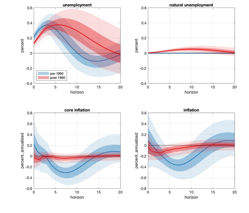
Figure 3.3. Forecasts of all variables, conditional on unemployment following the
path in the first subplot. The conditional forecasts are from the baseline VAR described
in section 2.2, augmented with long-term inflation expectations and the federal funds
rate. The solid lines are posterior medians, while the shaded areas correspond to 68- and
95-percent posterior credible regions. The pre- and post-1990 samples consist of data
from 1964:II to 1989:IV, and from 1989:I to 2019:III, respectively.
in the business cycle dynamics of inflation before and after 1990 stands out compared to
that of all the real variables that we have considered. Second, the co-movement of these
real variables is remarkably similar before and after 1990. Together, these two observations
suggest that we can focus the rest of the analysis on the bi-variate relationship between
inflation and real activity, with no need to be more specific on its measurement. As illus-
trated in section 4, however, this significant narrowing of the scope of the inquiry is not
sufficient to conclude that the anemic response of inflation to the cycle is due to a flatteningWHAT’S UP WITH THE PHILLIPS CURVE? 19
of the structural Phillips curve. The reason is that a flattening of the aggregate demand
relationship, perhaps induced by a more forceful reaction of monetary policy to inflation,
could in principle result in more stable inflation. Further distinguishing between these two
possibilities requires putting more structure on the problem, as we will then do in sections
5 and 6.
4. Lessons from a Stylized Model
To aid in the interpretation of the empirical facts described in section 3, we now introduce
a stylized model of the joint determination of inflation and real activity. This model,
which is directly inspired by McLeay and Tenreyro (2019), is based on the textbook New-
Keynesian framework of Woodford (2003) and Galí (2015). However, its implications for
the nature of business cycles under alternative hypotheses regarding the possible sources of
inflation stability are quite general, as we argue below. We use this simple model to make
three essential points: (i) the empirical facts of section 3 are consistent with two possible
explanations of the stability of inflation after 1990: either a reduction in the sensitivity of
pricing decisions to marginal cost pressures, or a change in the conduct of monetary policy;
(ii) the key implication that differs across these two hypotheses is that real activity is driven
predominantly by demand-type shocks in the first case, and supply-type disturbances in
the second; (iii) unfortunately, it is difficult to empirically verify which shocks—demand or
supply—are prevalent in the post-1990 period based on the co-movement pattern between
inflation and real activity, because the variation of inflation is minimal. Therefore, in the
next sections we will introduce more information and structure to further sharpen our
inference.
4.1. A simple model of aggregate demand and supply. The stylized model we con-
sider consists of the following three familiar equations:
(4.1) ⇡t = Et ⇡t+1 + (xt + st )
(4.2) xt = Et xt+1 (it Et ⇡t+1 t)
(4.3) it = Et ⇡t+1 + ↵ t + ⇡ ⇡t ,WHAT’S UP WITH THE PHILLIPS CURVE? 20
where ⇡t represents price inflation, xt ⌘ yt ytn is the output gap (defined as the log
deviation of output from a measure of potential), it is the nominal interest rate, and st
and t are exogenous disturbances. In this formulation, Et ⇡t+1 and Et xt+1 denote rational
expectations of next period’s inflation and output gap.15
Equation (4.1) is the model’s structural Phillips curve, an aggregate supply relationship
that maps higher output gaps into higher inflation. It is based on the dependence of
inflation on firms’ marginal costs—a fairly general feature of optimal pricing problems
(Sbordone, 2002)—in combination with some simplifying assumptions that make marginal
costs proportional to the output gap. These simplifying assumptions, however, are not
restrictive for our analysis, given that facts 3 and 4 in section 3 document a stable dynamic
relationship between many real activity variables usually employed to measure slack, such
as unemployment, hours, GDP and unit labor costs. Therefore, given this stability, we do
not need to take a strong stance on what xt precisely represents in our stylized model, and
will simply refer to it generically as real activity, or the output gap. Finally, the supply, or
cost-push shock (st ) in equation (4.1) stems from fluctuations in desired markups, which
explains why it is scaled by the slope .16
The other two equations constitute the demand block of the model. In particular, equa-
tion (4.2) is an Euler equation, or dynamic IS equation, which connects the nominal interest
rate to real activity. The strength of this negative relationship is governed by the parameter
> 0. In addition, the equation is perturbed by the shock t, which can be interpreted
as capturing fluctuations in the Wicksellian natural rate of interest or, more generally, as
a demand disturbance. Equation (4.3) is a simple interest rate rule that represents the
response of the monetary policy authority to economic developments. This specification
allows for a direct response of the policy rate to the IS shock—for reasons that will become
clear shortly—and to inflation, where the Taylor principle requires ⇡ > 0. Adding a term
15Lowercase letters denote logs, so that, for instance, y ⌘ log Y , where Y is the level of output. Y n is
t t t t
natural output, the level of output that would be observed in the absence of nominal rigidities.
16Under Calvo pricing, fluctuations in desired markups have the same effect on inflation as those in real
marginal costs. Therefore, in the limit in which prices never change, the sensitivity of inflation to both real
activity and desired markups captured by the parameter goes to zero and inflation becomes perfectly
stable. More generally, we could allow for other sources of exogenous supply shocks, which might include, for
instance, exogenous shifts in inflation expectations that are not fully captured by the rational expectations
term Et ⇡t+1 . In the presence of such shocks, the variability of inflation is not zero even when = 0, but
the qualitative implications of the model described below do not change.WHAT’S UP WITH THE PHILLIPS CURVE? 21
in the output gap, as in Taylor (1993), or a monetary policy shock would not change the
model’s key qualitative implications.
Plugging the policy rule into the IS equation produces a negative relationship between
inflation and real activity of the form
⇡t = (xt Et xt+1 dt ) ,
1
where ⌘( ⇡) 0 and dt ⌘ (↵ 1) t is a simple re-scaling of the demand shock.
If the demand disturbance is observable, monetary policy can perfectly offset it by setting
↵ = 1. More generally, demand shocks are likely to be transmitted to the economy at least
partially, either because the monetary authority observes them with noise, or because it
chooses not to react to them fully, or because it is prevented from doing so by the zero
lower bound. All of these scenarios are captured in this model by ↵ < 1, which implies
some pass-through of these shocks into inflation.
The negative slope of this aggregate demand equation reflects the fact that monetary
policy leans against inflation by raising the real interest rate, which in turns lowers real
activity. This feature of aggregate demand does not depend on the exact specification of the
interest rate rule, as long as the real interest rate responds positively to inflation. As shown
by McLeay and Tenreyro (2019), this is also a feature of aggregate demand under optimal
monetary policy. In this respect, our approach to modeling monetary policy and that of
McLeay and Tenreyro (2019) are isomorphic, even if they derive the aggregate demand
equation directly from an optimal policy problem, without relying on the IS equation. In
comparison, our setup with an IS equation and a policy rule is more explicit about some
potential sources of demand shocks, but its key implications are the same.
In sum, at a high level of generality, the model is just an aggregate supply (AS) and ag-
gregate demand (AD) framework, similar to those typically found in intermediate macroe-
conomics textbooks, such as Jones, 2020. In fact, most of the intuition that we derive
from this framework stems exactly from this underlying demand and supply structure, as
in McLeay and Tenreyro (2019).
4.2. Two alternative sources of inflation stabilization. Given the structure of the
model, it is immediate to see that stable inflation can be the result of at least two changes
in the economy. First, a flat structural Phillips curve, which corresponds to ! 0. Second,WHAT’S UP WITH THE PHILLIPS CURVE? 22 a very elastic aggregate demand curve, which corresponds to ! 0 or, in terms of the interest rate rule, to ⇡ ! 1. In what follows, we will take these two extreme parametric restrictions as stylized representations of the two alternative hypotheses on the ultimate source of the observed inflation stability that have been most discussed in the literature.17,18 The first hypotheses—the (Phillips curve) slope hypothesis, for short—is that inflation is stable because changes in the structure of goods markets or in firms’ pricing practices have produced a structural disconnect between inflation and marginal cost pressures. The literature has explored many mechanisms that might lead to such a disconnect, as reviewed in the introduction. Distinguishing among them is beyond the scope of this paper. The second hypothesis that we focus on—the policy hypothesis, for short—is that inflation is stable because monetary policy now leans more heavily against inflation than it did in the first part of the sample, thus reducing its variability in equilibrium. This is the hypothesis favored by McLeay and Tenreyro (2019). In our stylized model, this hypothesis amounts to assuming that ⇡ has increased in the second part of the sample. In the limit with ⇡ ! 1, inflation becomes perfectly stable. In practice, there are many channels through which a change in the actual conduct of monetary policy and in the communication and public understanding of its objectives can affect inflation dynamics and inflation expectations, without going to the extreme of promising a very large increase in policy rates in reaction to even small changes in inflation.19 17In our stylized model, a flat aggregate demand curve could also result from ! 1, although its intercept (and thus inflation) would still depend on the demand shock in this case. We do not focus on this possibility because there is not much evidence that the responsiveness of the real economy to interest rates has increased since 1990. If anything, there is some discussion of a reduced pass-through of interest rates, and of financial conditions more generally, onto real variables, especially since the financial crisis. 18Another obvious possibility is that the volatilities of both shocks have fallen dramatically. Although the large literature on the Great Moderation indeed suggests that the volatility of (at least some) shocks did fall in the mid 1990s, we do not focus on this possible explanation because the volatility of real variables has not fallen nearly as much as that of inflation, at least in response to business cycle shocks. In this respect, our main object of inquiry is the reduction in the volatility of inflation relative to that of its plausible real drivers, conditional on business cycle shocks. 19Inflation expectations do not play a crucial independent role in our model because under rational ex- pectations they are a function of the same shocks that drive inflation. In this respect, stable inflation and inflation expectations are two manifestations of the same phenomenon. Carvalho et al., 2019 discuss the notion of expectation anchoring theoretically and empirically in the context of a model with learning, in which expectations are not as tightly linked to actual inflation as under rational expectations. Jorgensen and Lansing, 2019 also study the implications of a learning model for the observed connection between inflation and real activity.
You can also read