Warm Magnets - CAS CERN - CERN Indico
←
→
Page content transcription
If your browser does not render page correctly, please read the page content below

Warm Magnets
CAS Chavannes de Bogis, 28-Sept-2021, warm magnets, GdR

 Gijs de Rijk
 CERN

 CAS

 Chavannes de Bogis, Switzerland
 28th September 2021

 1

Copyright statement and speaker’s release for video publishing
CAS Chavannes de Bogis, 28-Sept-2021, warm magnets, GdR

 The author consents to the photographic, audio and video recording of this lecture
 at the CERN Accelerator School. The term “lecture” includes any material
 incorporated therein including but not limited to text, images and references.

 The author hereby grants CERN a royalty-free license to use his image and name as
 well as the recordings mentioned above, in order to post them on the CAS
 website.

 The author hereby confirms that to his best knowledge the content of the lecture
 does not infringe the copyright, intellectual property or privacy rights of any third
 party. The author has cited and credited any third-party contribution in
 accordance with applicable professional standards and legislation in matters of
 attribution. Nevertheless the material represent entirely standard teaching
 material known for more than ten years. Naturally some figures will look alike
 those produced by other teachers.
 2

Contents

 • Introduction: magnetic field and warm magnet principles
CAS Chavannes de Bogis, 28-Sept-2021, warm magnets, GdR

 • Field description and magnet types
 • Practical magnet design & manufacturing
 • Permanent magnets
 • Examples of accelerator magnets from the early times until
 the present
 • Literature on warm Magnets

 3
Magnet types, technological view

 We can also classify magnets based on their technology
CAS Chavannes de Bogis, 28-Sept-2021, warm magnets, GdR

 electromagnet permanent magnet

 iron dominated coil dominated

 normal conducting
 superconducting
 (resistive)

 cycled / ramped
 static fast pulsed
 slow pulsed
 4
Earth magnetic field

 In Geneva, on 06/09/2021, the (estimated) magnetic field (flux density) is
 |B| = 47672 nT = 0.047672 mT = 4.7672·10-5 T ≈ 0.5 Gauss. Bhorizontal = 22259 nT
CAS Chavannes de Bogis, 28-Sept-2021, warm magnets, GdR

 5
Maxwell equations

 Integral form Differential form

CAS Chavannes de Bogis, 28-Sept-2021, warm magnets, GdR

 ර Ԧ = න Ԧ + Ԧ Ampere’s law = Ԧ +

 ර Ԧ = − න Ԧ Faraday’s equation = −

 න Ԧ = 0 Gauss’s law for = 0
 magnetism

 න Ԧ = න =

 Gauss’s law

 With: = = 0 = 0 +

 = = 0 +
 Ԧ = + .
 6
Magnetostatics

 Let’s have a closer look at the 3 equations that describe
 magnetostatics
CAS Chavannes de Bogis, 28-Sept-2021, warm magnets, GdR

 Gauss law of
 magnetism
 (1) div = 0 always holds

 Ampere’s law with no
 time dependencies
 (2) rot = Ԧ holds for magnetostatics

 Relation between
 field and the flux (3) = 0 holds for linear materials
 density

 7
Magnetic fields

 From Ampere’s law with no time
 dependencies (Integral form) ò C
 B × dl = m0 I encl.
CAS Chavannes de Bogis, 28-Sept-2021, warm magnets, GdR

 We can derive the law of Biot and Savart
 m0 I
 B= ĵ
 2p r

 If you wanted to make a B = 1.5 T magnet
 with just two infinitely thin wires placed at
 100 mm distance in air one needs :
 I = 187500 A
 • To get reasonable fields ( B > 1 T) one
 needs large currents
 • Moreover, the field homogeneity will be
 poor
 8
Iron dominated magnets

 With the help of an iron yoke
 we can get fields with less
 ò C
 H × dl = N × I
 current
 N × I = H iron × liron + H airgap × lairgap Þ
CAS Chavannes de Bogis, 28-Sept-2021, warm magnets, GdR

 B B
 N ×I = × liron + × lairgap Þ
 Example: C shaped dipole for
 accelerators
 m0mr m0
 lairgap × B This is valid as mr >> 1 in
 N ×I =
 Yoke
 m0 the iron : limited to B < 2 T

 coil

 B = 1.5 T mr as func on of B for low carbon magnet steel
 (Magne l BC)
 Gap = 50 mm 9000
 8000
 N . I = 59683 A 7000
 6000
 mr 5000
 2 x 30 turn coil 4000
 I = 994 A 3000
 2000

 @5 A/mm2, 200 mm2 1000
 0
 0 0.5 1 1.5 2
 14 x 14 mm Cu B (T) 9

Comparison : iron magnet and air coil

 Imagine a magnet with a 50 mm vertical gap ( horizontal width ~100 mm)
 Iron magnet wrt to an air coil:
 – Up to 1.5 T we get ~6 times the field
CAS Chavannes de Bogis, 28-Sept-2021, warm magnets, GdR

 – Between 1.5 T and 2 T the gain flattens of : the iron saturates
 – Above 2 T the slope is like for an air-coil: currents become too large to use
 resistive coils
 8

 7

 6

 5
 B [T]

 4
 These two curves are the
 3
 transfer functions – B field vs.
 current – for the two cases 2
 with iron

 1 without iron
 iron, infinite permeability
 0
 0 100 200 300 400 500 600 700 800 900 1000
 NI [kA]
 Courtesy A. Milanese, CERN 10
Magnetic field quality: multipole description ∞ −1 −4 + + = 10 1 ൫ + ) =1 CAS Chavannes de Bogis, 28-Sept-2021, warm magnets, GdR ℎ: = + , ℎ ℎ , ℎ ℎ , 1 ℎ ℎ , ℎ ℎ , ℎ ℎ . The “wanted” or is equal to 1 In a ring-shaped accelerator, where the beam does multiple passes, one typically demands : , ≤ 1 10−4 11
Magnetic Length

 In 3D, the longitudinal dimension of the magnet is described by a magnetic length
CAS Chavannes de Bogis, 28-Sept-2021, warm magnets, GdR

 ∞

 0 = න
 −∞

 lmag

 Courtesy A. Milanese, CERN

 magnetic length Lmag as a first approximation:
 • For dipoles Lmag = Lyoke + d d = pole distance
 • For quadrupoles: Lmag = Lyoke + r r = radius of the inscribed circle
 between the 4 poles
 12
Magnets in an accelerator: power convertor and
 circuit

 Cu (or Al) B (flux density)
 cables or
 busbars
CAS Chavannes de Bogis, 28-Sept-2021, warm magnets, GdR

 beam
 power
 Convertor
 (current
 Vacuum
 source)
 chamber

 • B field stability in time: ~10-5 - 10-6 Cu or Al coil Steel yoke

 • Typical R of a magnet ~20mW - 60mW
 Then the Power Convertor has to
 • Typical L of a magnet ~20mH – 200mH
 Supply : 0-500 A with a stability of
 • Powering cable (for 500A): Cu 250 mm 2
 a few ppm.
 (Cu: 17 nW.m) R = 70 mW/m, for 200m:
 Voltage up to 40 V (resitive)
 R= 13mW
 And 100 V (inductive)
 • Take a typical rise time 1s
 13
Types of magnetic fields for accelerators
CAS Chavannes de Bogis, 28-Sept-2021, warm magnets, GdR

 Courtesy D. Tommasini, CERN
 14
fluxlines in magnets

 Dipole Quadrupole sextupole
CAS Chavannes de Bogis, 28-Sept-2021, warm magnets, GdR

 0 0.8 1.6 0 0.8 1.6 0 0.5 1.0
 T T T T T T

 15
Symmetry and allowed harmonics

 In a fully symmetric magnet certain field harmonics are natural.
CAS Chavannes de Bogis, 28-Sept-2021, warm magnets, GdR

 Magnet type Allowed harmonics bn
 n=1 Dipole n=3,5,7,...
 n=2 Quadrupole n=6,10,14
 n=3 Sextupole n=9,15,21
 n=4 Octupole n=12,20,28

 Non-symmetric designs and fabrication errors give rise to non allowed
 harmonics: bn with n other than listed above and an with any n

 NB: For “skew” magnets this logic is inverted !

 16
CAS Chavannes de Bogis, 28-Sept-2021, warm magnets, GdR

Courtesy D. Tommasini, CERN
 Basic magnet types

 17
Practical magnet design & manufacturing

 Steps in the process:
CAS Chavannes de Bogis, 28-Sept-2021, warm magnets, GdR

 1. Specification
 2. Conceptual design
 3. Detailed design
 1. Yoke: yoke size, pole shape, FE model optimization
 2. Coils: cross-section, geometry, cooling
 3. Raw material choice
 4. Yoke ends, coil ends design
 4. Yoke manufacturing, tolerances, alignment, structure
 5. Coil manufacturing, insulation, impregnation type
 6. Magnetic field measurements

 18
Specification Before you start designing you need to get from the accelerator designers: • B(T) or G (T/m) (higher orders: G3(T/m2), etc) • Magnet type: C-type, H-type, DC (slow ramp) or AC (fast ramp) CAS Chavannes de Bogis, 28-Sept-2021, warm magnets, GdR • Aperture: – Dipole : “good field region“ airgap height and width – Quads and higher order: “good field region“ aperture inscribed circle • Magnetic length and estimated real length • Current range of the power convertor (and the voltage range: watch out for the cables ) • Field quality: ∆ ∆ : , : , = 1,2,3,4,5, … • Cooling type: air, water (Pmax , Dpmax and Qmax (l/min)) • Jacks and Alignment features • Vacuum chamber to be used fixations, bake-out specifics These need careful negotiation and often iteration after conceptual (and detailed) design, and will probably be a compromise. 19
Conceptual design

 • From B and l you get NI (A)
 = Yoke
 0 Wyoke
 Wpole
 • From NI (A) and the power convertor Imax you 1
CAS Chavannes de Bogis, 28-Sept-2021, warm magnets, GdR

 NI coil
 2
 get N
 • Then you decide on a coil X-section using: Wyoke B
 = 5 ൗ 1
 2 2
 NI

 = 1 Τ 2
 • This defines the coil cavity in the yoke (you
 add 0.5 mm insulation around each conductor
 and 1 mm ground insulation around the coil)
 and select the best fitting rectangular
 • You can the draw the draft X-section using:

 = ℎ 1.5 < < 2

 • Decide on the coil ends: racetrack, bedstead
 • You now have the rough magnet cross section
 and envelope

 20
Power generated

 Power generated by coil
 • DC: from the length of the conductor N∙Lturn , the cross-section s and the
 specific resistivity r of the material one gets the spent Power in the coil
CAS Chavannes de Bogis, 28-Sept-2021, warm magnets, GdR

 = 1.72 1 + 0.0039 − 20 10−8 Ω
 Τ Τ = 2 ℎ: = 2.65 1 + 0.0039 − 20 10−8 Ω

 For AC: take the average I2 for the duty cycle

 Power losses due to hysteresis in the yoke: (Steinmetz law up to 1.5 T)
 Τ = 1.6 ℎ = 0.01 0.1, ≈ 0.02

 Power losses due to eddy currents in the yoke
 2
 Τ = 0.05 10
 with the lamination thickness in mm, ℎ

 Courtesy D. Tommasini, CERN 21
Cooling circuit parameters

 Aim: to design dcooling , Pwater[bar], DP[bar], Q[l/min]

 Choose a desired DT
CAS Chavannes de Bogis, 28-Sept-2021, warm magnets, GdR

 • (20ºC or 30ºC depending on the Tcooling water )

 • with the heat capacity of water (4.186 kJ/kgºC) we now know the required water
 flow rate: Q(l/min)

 • The cooling water needs to be in moderately turbulent regime (with laminar flow
 the flow speed is zero on the wall !): Reynolds > 2000

 = ~ 140 Τ ~40°

 • A good approximation for the pressure drop in smooth pipes can be derived
 from the Blasius law, giving:
 Τ 1.75
 Δ = 60
 4.75
 Courtesy D. Tommasini, CERN 22
Theoretical pole shapes

 The ideal poles for dipole, quadrupole, sextupole, etc. are lines of constant
 scalar potential
CAS Chavannes de Bogis, 28-Sept-2021, warm magnets, GdR

 Dipole = ±ℎ/2 straight line

 quadrupole 2 = ± 2 hyperbola

 sextupole 3 2 − 3 = ± 3

 23
Practical pole shapes: shims and alignment features

 • Dipole example: below a lamination
 of the LEP main bending magnets,
 with the pole shims well visible
CAS Chavannes de Bogis, 28-Sept-2021, warm magnets, GdR

 • Quadrupoles: at the edge of the pole one can
 put a combination a shim and alignment feature
 (examples: LHC-MQW, SESAME quads, etc)
 • This then also allows to measure the pole
 distances : special instrumentation can be made
 for this
 24
Finite Element electromagnetic models

 • Aim of the electromagnetic FE models:
 – The exact shape of the yoke needs to be designed
 • Optimize field quality: adjust pole shape, minimize high saturation
CAS Chavannes de Bogis, 28-Sept-2021, warm magnets, GdR

 zones
 • Minimize the total steel amount ( magnet weight, raw material cost )
 – Calculate the field: needed for the optics and dynamic aperture modelling
 • transfer function Bxsection(I) , න , magnetic length
 • multipoles (in the centre of the magnet and integrated) bn and an

 • Some Electromagnetic FE software packages that are often used:
 – Opera from Cobham: 2D and 3D commercial software see:
 http://operafea.com/
 – “Good old” Poisson, 2D: now distributed by LANL-LAACG see:
 http://laacg.lanl.gov/laacg/services/download_sf.phtml
 – ROXIE (CERN) 2D and 3D, specialized for accelerator magnets; single fee
 license for labs & universities see: ttps://espace.cern.ch/roxie/default.aspx
 – ANSYS Maxwell: 2D and 3D commercial software
 see: http://www.ansys.com/Products/Electronics/ANSYS-Maxwell
 25
FE models: steel curves

 You can use a close ‘generic’ B(H) curve for a first cut design
 You HAVE to use a measured, and smoothed, curve to properly calculate
 Bxsection(I) , න , bn and an
CAS Chavannes de Bogis, 28-Sept-2021, warm magnets, GdR

 As illustration the curves for several types of steel:
 2.5
 End slope is m0

 2

 1.5
 B(T)

 Magnetil LAF 1.5 mm
 1 Iron AC37
 St-Petersburg 0.75 mm
 ISR 1.5 mm

 slope is mrm0 steel Ru 21848
 Si 3.25%
 0.5
 Magnetil LAC 1.5 mm

 0
 0 5000 10000 15000 20000 25000 30000 35000
 H (/m) 26
Yoke shape, pole shape: FE model optimization

 Use symmetry and the thus appropriate boundary
 conditions to model only ¼th (dipoles, quadrupoles )
 or even 1/6th sextupoles.
CAS Chavannes de Bogis, 28-Sept-2021, warm magnets, GdR

 Meshing needs attention in the detailed areas like
 poles, slits, etc

 27
Yoke manufacturing

 • Yokes are nearly always laminated to reduce eddy currents during ramping
 • Laminations can be coated with an inorganic (oxidation, phosphating, Carlite) or
 organic (epoxy) layer to increase the resistance
CAS Chavannes de Bogis, 28-Sept-2021, warm magnets, GdR

 • Magnetic properties: depend on chemical composition + temperature and
 mechanical history
 • Important parameters: coercive field Hc and the saturation induction.
 – Hc has an impact on the remnant field at low current
 • Hc < 80 A/m typical
 • Hc < 20 A/m for magnets ranging down also to low field B < 0.05 T
 – low carbon steel (C content < 0.006%) is best for higher fields B > 1 T
 Field Strength [A/m] Minimum Field Strength H Minimum
 Induction [T] Example [A/m] Induction B [T] Example
 40 0.20 specification for 100 0.07 specification for
 60 0.50 1.5 mm thick 300 1.05 0.5 mm thick
 120 0.95
 oxide coated 500 1.35 epoxy coated
 500 1.4
 1 200 1.5
 steel for the LHC 1000 1.50 steel for LHC
 2 500 1.62 warm separation 2500 1.62 transfer line
 5000 1.72
 5 000 1.71 magnets, corrector magnet
 10000 1.82
 10 000 1.81 Bmax= 1.53 T Bmax=0.3 T
 24 000 2.00
 28
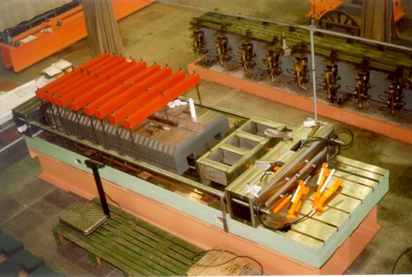
Yoke manufacturing

 Stacking an MBW dipole yoke stack Stacking an MQW quadrupole yoke stack
CAS Chavannes de Bogis, 28-Sept-2021, warm magnets, GdR

 MQW yoke assembly

 29
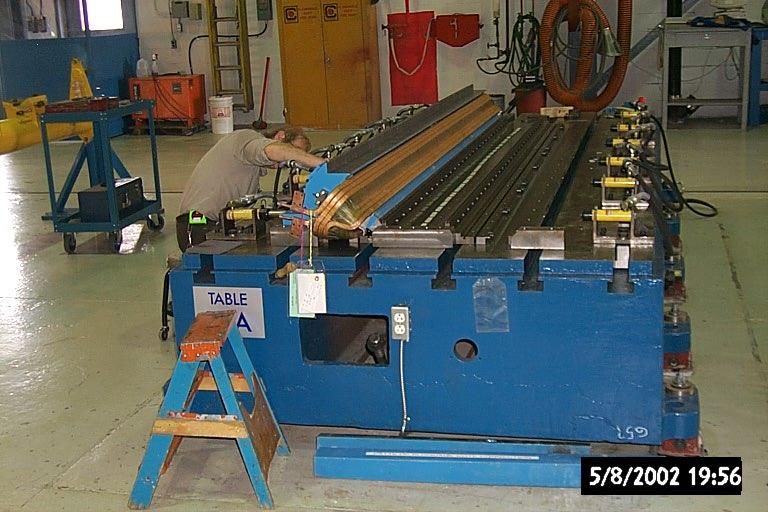
Yoke stack manufacturing

 Double aperture LHC quadrupole MQW
 Stacking on a precision table
CAS Chavannes de Bogis, 28-Sept-2021, warm magnets, GdR

 Welding the structural plates

 Finished stack

 30
Yokes: holding a laminated stack together

 • Yokes are either
 – Glued , using epoxy coated laminations
 – Welded, full length plates are welded on the outside
CAS Chavannes de Bogis, 28-Sept-2021, warm magnets, GdR

 Corrector dipole in TI2 and TI8 LHC injection lines
 – Compressed by tie rods in holes
 Magnet with gluedoflaminated
 or a combination all these yokes assembled with bolts.
 • To be able to keep the yoke (or yoke stack) stable you probably need end
 plates (can range from ± 1 cm to 5 cm depending on the size)
 • The end plates have pole chamfers and often carry end shims
 Glued yoke (MCIA LHC TL)
 Welded stack

 Tie rod

 Main parameters
 Name MCIA V
 Type Vertical correcting dipole
 Nominal peak field [T] 0.26
 Imax [A] 3.5
 N. Of turns 1014
 Résistance [Ω] 13.9
 Yoke lenght [mm] 450
 Gap [mm] 32.5
 Total weight [kg] 300 31
Coil manufacturing, insulation, impregnation type

 • Winding Cu conductors is an well established technique
 • When the Cu conductor is thick it is best to use “dead soft” Cu (T treatment)
 • Insulation of the coil
CAS Chavannes de Bogis, 28-Sept-2021, warm magnets, GdR

 – Glass fibre – epoxy impregnated
 • Individual conductor 0.5 mm glass fibre, 0.25 mm tape wound half
 lapped
 • Impregnated with radiation resistant epoxy, total glass volume ratio
 >50%
 – For thin conductors: Cu emanel coated, possibly epoxy impregnated
 afterwards

 32
Coil ends

 For dipoles some main types are racetrack of bedstead
CAS Chavannes de Bogis, 28-Sept-2021, warm magnets, GdR

 Quadrupoles

 33
Coil manufacturing

 MQW Glass fibre tape wrapping.
CAS Chavannes de Bogis, 28-Sept-2021, warm magnets, GdR

 Winding the hollow Cu
 conductor

 34
Coil manufacturing

 Mounted coil coil electrical test (under water !)
CAS Chavannes de Bogis, 28-Sept-2021, warm magnets, GdR

 Dipoles racetrack coil
 MBXW Coil winding

 Finished MBXW coil

 35
Magnetic field measurements

 Several Magnetic Measurements techniques can be applied, e.g.:
 • Rotating coils: multipoles and integrated field or gradient in all magnets
 • Stretched wire: magnetic centre and integrated gradient for n > 1 magnets
CAS Chavannes de Bogis, 28-Sept-2021, warm magnets, GdR

 • Hall probes: field map
 • Pickup coils: field on a current ramp
 • Example below : MQW : double aperture quadrupole for the LHC.

 The radial coil
 Mole assembly 1
 Flux in a Radial Coil:
 R2
 F(q ) = NL ò Bq (r ,q )dr Y
 R1

 q = q 0 + wt B

 AS Budapest, 7-Oct-2016, warm magnets, GdR
 Mole Assembly
 R2 Side View
 Induced Voltage: R1 X
 Gravity
 Sensor
 Pneumatic
 Break
 Incremental
 Encoder
 Slip Rings Harmonic
 Coils

 æ ¶F ö
 V (t ) = -ç ÷
 è ¶t ø
 Integrated Voltage:
 Mole Assembly Top View 36
 Rotating radial coil
 Cross section of a radial coil
Sextupoles

 • These are sextupoles (with embedded correctors) of the main ring of the
 SESAME light source
CAS Chavannes de Bogis, 28-Sept-2021, warm magnets, GdR

 Courtesy A. Milanese, CERN 37
Permanent magnets

 Linac4 @ CERN permanent magnets , quadrupoles
CAS Chavannes de Bogis, 28-Sept-2021, warm magnets, GdR

 Permanent Magnets : LINAC 4
 DTL tank

 Pictured : Cell-Coupled Drift Tube Linac module.

 • Permanent magnet because of space between DTL tanks
 • Sm2Co17 permanent magnets
 • Integrated gradient of 1.3 to 1.6 Tesla
 • 15 magnets
 • Magnet length 0.100 m
 • Field quality/amplitude tuning blocks

 Courtesy D. Tommasini, CERN Sextupole Hallback Array 38
 Introduction to accelerator physics Varna, 19 September, 1 October 2010 Davide Tommasini : Magnets (warm)25
Hybrid magnets

 CLIC final focus, Hybrid Magnets : CLIC final focus
CAS Chavannes de Bogis, 28-Sept-2021, warm magnets, GdR

 Gradient: > 530 T/m
 Aperture Ø: 8.25 mm
 Tunability: 10-100%

 Courtesy D. Tommasini, CERN 39
 Introduction to accelerator physics Varna, 19 September, 1 October 2010 Davide Tommasini : Magnets (warm)
CAS Chavannes de Bogis, 28-Sept-2021, warm magnets, GdR

 Examples;

 Some history, some modern regular magnets and some
 special cases

 40
The 184’’ (4.7 m) cyclotron at Berkeley (1942)
CAS Chavannes de Bogis, 28-Sept-2021, warm magnets, GdR

 Courtesy A. Milanese, CERN 41
Cyclotrons
CAS Chavannes de Bogis, 28-Sept-2021, warm magnets, GdR

 A modern synchrocyclotron for medical application –
 IBA S2C2
 Harvard 1948
 ® at the same energy synchrocyclotrons can be build more compact and with lower
 cost than sector cyclotrons; however, the achievable current is significantly lower

 energy 230 MeV Feb/2013, courtesy:
 current 20 nA P.Verbruggen,IBA
 dimensions Æ2.5 m x 2 m
 weight < 50 t
 extraction radius 0.45 m
 s.c. coil strength 5.6 Tesla
 RF frequency 90…60 MHz
 repetition rate 1 kHz
 1974

 20
 42
Some early magnets (early 1950-ies)

 Bevatron
 (Berkeley)
CAS Chavannes de Bogis, 28-Sept-2021, warm magnets, GdR

 1954, 6.2 GeV

 Cosmotron
 (Brookhaven)
 1953, 3.3 GeV
 Aperture:
 20 cm x 60 cm

 43
No. of non-linear lenses 20 pairs Harmonic number 20
 Frequency range 2.9–9.55 MHz
 PS combined function dipole Power per cavity 6 kW

 Magnet and Power Supply

 Magnetic field: Injection
 at injection 147 G
 for 24.3 GeV 1.2 T Injection energy 50 ± 0.1 MeV
CAS Chavannes de Bogis, 28-Sept-2021, warm magnets, GdR

 maximum 1.4 T Injection field 147 G
 Weight of one magnet unit 38 t Length of linear accelerator 30 m
 Total weight
 Gradient @1.2ofT coils (alumin.)
 : 5 T/m 110 t RF power 5 MW at 202.5 MH
 Total weight of iron 3400 t during 200 ms
 Rise timewith
 Equipped to 1.2 T
 pole-face 1s
 windings
 No. for higher
 of cycles order (1.2 T
 per minute Fig. 10: Model with movable plates to determine final Fig. 11: The ‘n’ values of open and c
 Water cooled Al race- profile. the remanent field show
 corrections
 operation) 20
 track coils Vacuum System difference. The acceptab
 thickness determined e xperim
 Peak power to energize the The final form of the magnet block is given in Fig. 12. The construction of the 1
 magnet 34 600 kW Vacuum chamber length
 entrusted to Ansaldo Fig. 9: Final
 in Genoa with pole
 steel profile. 628
 laminations produced mnearby fact
 in the
 (Fig. 13). Ansaldo won the contract because of the higher precision of their punching
 Stored energy 107 J Vacuum chamber
 with those madesection
 by other European manufacturers. 7 ´ 14 cm
 Paying extreme attention to tolerances and in general to very sound engineer
 Mean dissipated power 1500 kWcomponent was,Wall thickness
 I believe, (stainless
 of capital importance steel)
 not only for the success 2 mm of the PS b
 Magnet gap at equilibrium orbit Vacuumat pumps
 10 cm subsequent machines (ø 10 cm) 4
 CERN. It taught all of us how to tackle technical design and+ 67 stations
 the basis of Pressure,
 an attitude better
 which was thanone of the facets of J. B. Adams’s 10–5 mmHg personality
 pessimism’, just the opposite of ‘blind optimism’. Indeed John was a pessimist not in
 but in the sense that he believed that Nature had no reason to make gifts to accel
 Therefore the correct attitude consisted in understanding the finest details of each pro
 make a design leaving nothing to chance on the way to success. Some people co
 conservatism and overcautiousness. But how can one consider as conservative o
 extraordinary engineers of our time, a man who undertook to construct the first proton
 in the world, the first underground large accelerator and, finally, the first pp collider?
 Fig. 12: Final form of the magnet blocks.

 The apparent simplicity of the magnet system masked a fair degree of sophist
 many studies and a lot of experimental work. Complication
 Courtesy was due to:CERN 44
 D. Tommasini,
CPS booster

 PS Booster Magnets
 4 accelerator rings in a common yoke. (increase total beam intensity by 4 in
 presence of space charge limitation at low
 Spare energy):
 Booster Dipole B=1.48 T @Booster
 Installed 2 GeV
 Dipole
 1.4 GeV Magnet Cycle
 Was originaly designed for 0.8 GeV !
CAS Chavannes de Bogis, 28-Sept-2021, warm magnets, GdR

 32 Dipole magnets for Booster Ring
 Magnet Weight - 12000 Kg
 Core Length - 1537 mm ‘Thick’ End Plate
 Aperture - 103 mm BDL correction Windings
 Magnetic flux @ 1.4 GeV operation 1.064 T compensate the 1% difference between
 the inner and outer rings.
 Yoke construction:
 Laminated core stacked between Laminations
 ‘thick’ end plates assembled using
 external welded tie bars. Lamination
 insulation achieved through a
 phosphatizing process.
 Welded tie Bars
 Courtesy D. Tommasini, CERN
 Booster Ring
 4 Booster to PS
 LINAC to Booster 3
 2
 1 45
dipole magnet : SPS dipole
 CAS Chavannes de Bogis, 28-Sept-2021, warm magnets, GdR

 H magnet
s of bending magnets oftype MBB
 the SPS.
 B = 2.05 T
 Coil : 16 turns
 I max = 4900 A
 Aperture = 52 × 92 mm2
 L = 6.26 m
 Weight = 17 t

 46
Quadrupole magnet : SPS quadrupole
CAS Chavannes de Bogis, 28-Sept-2021, warm magnets, GdR

 type MQ
 G = 20.7 T/m
 Coil : 16 turns
 I max = 1938 A
 Aperture inscribed radius = 44 mm
 Lcoil = 3.2 m
 Weight = 8.4 t

 47
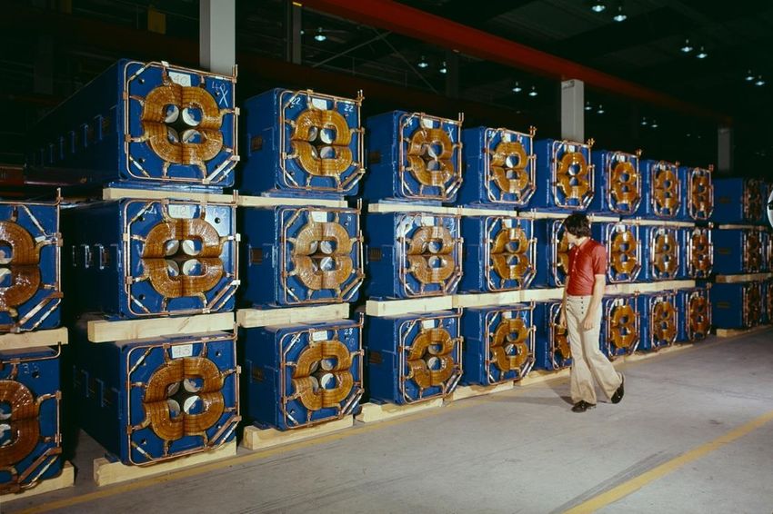
CAS Chavannes de Bogis, 28-Sept-2021, warm magnets, GdR
 MBW LHC warm separation dipole (1)

48
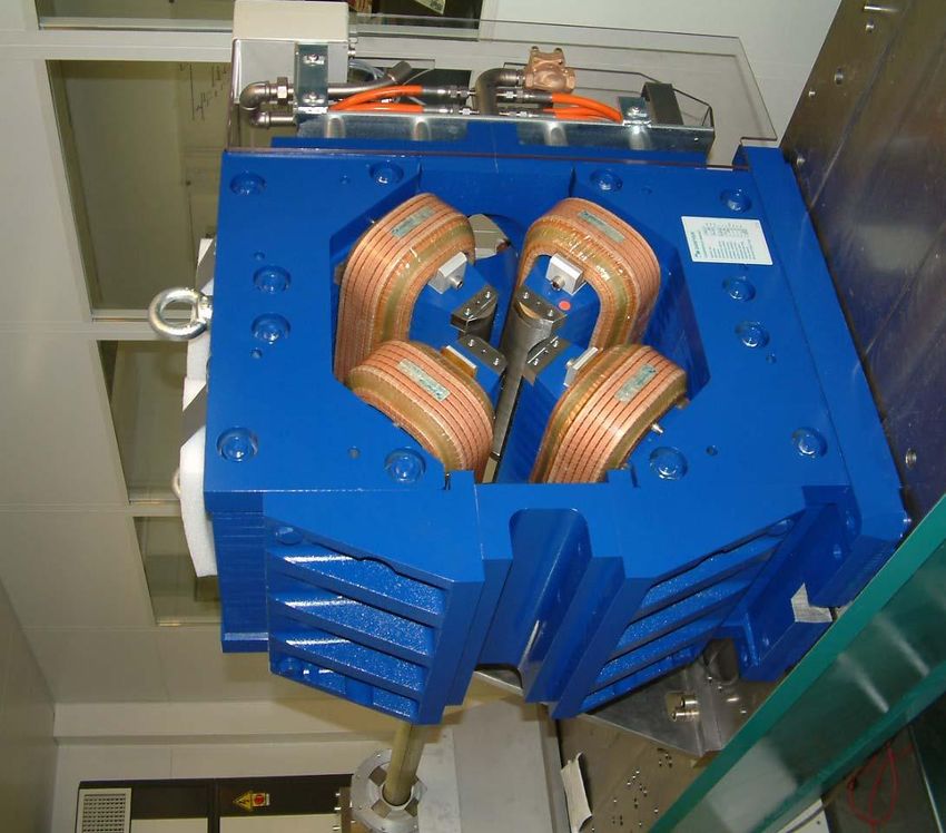
CAS Chavannes de Bogis, 28-Sept-2021, warm magnets, GdR
 MQW: LHC warm double aperture quadrupole

49
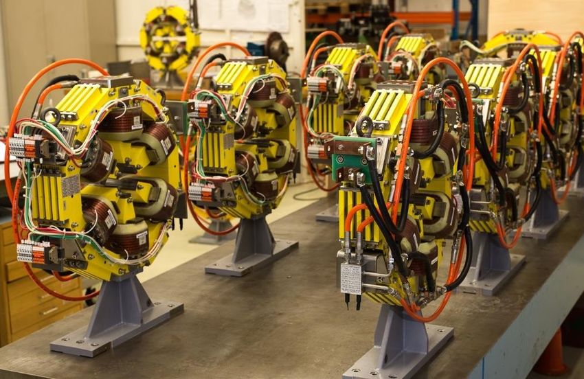
CAS Chavannes de Bogis, 28-Sept-2021, warm magnets, GdR

 •
 .
 Elena, anti proton decelerator

50
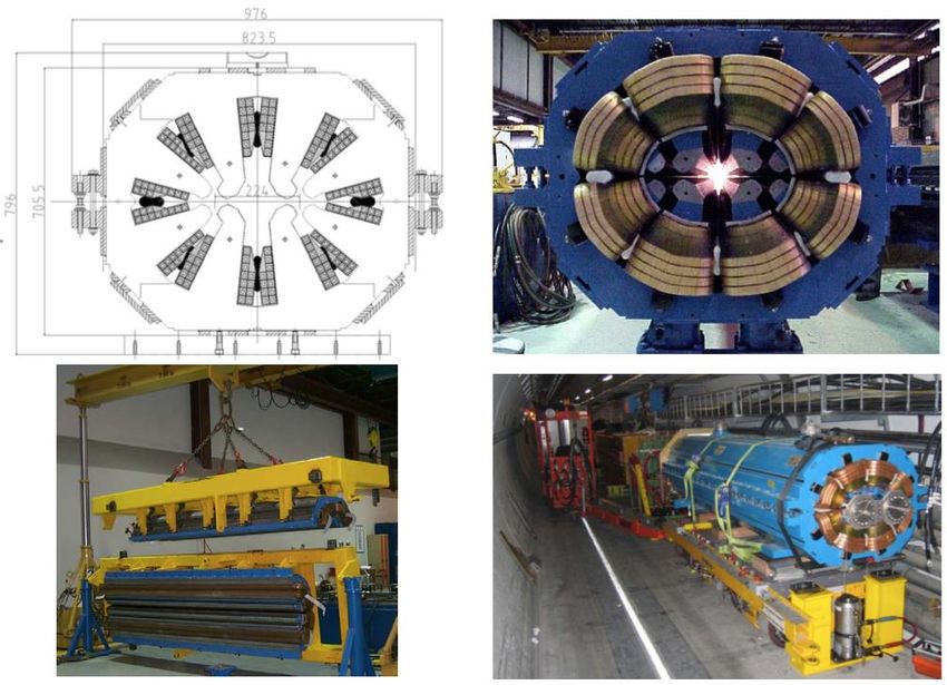
Soleil, synchrotron light-source
CAS Chavannes de Bogis, 28-Sept-2021, warm magnets, GdR

 Courtesy A. Dael, CEA
 51
Literature on warm accelerator magnets

 • Books
 – G.E.Fisher, “Iron Dominated Magnets” AIP Conf. Proc., 1987 -- Volume 153, pp.
 1120-1227
CAS Chavannes de Bogis, 28-Sept-2021, warm magnets, GdR

 – J. Tanabe, “Iron Dominated Electromagnets”, World Scientific, ISBN 978-981-256-
 381-1, May 2005
 – P. Campbell, Permanent Magnet Materials and their Application, ISBN-13: 978-
 0521566889
 – S. Russenschuck, Field computation for accelerator magnets : analytical and
 numerical methods for electromagnetic design and optimization / Weinheim : Wiley,
 2010. - 757 p.

 • Schools
 – CAS Bruges, 2009, specialized course on magnets, 2009, CERN-2010-004
 – CAS Frascati 2008, Magnets (Warm) by D. Einfeld
 – CAS Varna 2010, Magnets (Warm) by D. Tommasini

 • Papers and reports
 – D. Tommasini, “Practical definitions and formulae for magnets,” CERN,Tech. Rep.
 EDMS 1162401, 2011 52
Acknowledgements

 For this lecture I used material from lectures, seminars, reports, etc. from the many
 colleagues. Special thanks goes to:
 Davide Tommasini, Attilio Milanese, Antoine Dael, Stephan Russenschuck,
CAS Chavannes de Bogis, 28-Sept-2021, warm magnets, GdR

 Thomas Zickler

 And to the people who taught me, years ago, all the fine details about magnets !

 53
You can also read


