Visual anticipation of the future path: Predictive gaze and steering
←
→
Page content transcription
If your browser does not render page correctly, please read the page content below
Journal of Vision (2021) 21(8):25, 1–23                                                                                                                       1

          Visual anticipation of the future path: Predictive gaze and
          steering
                                                                                Cognitive Science, Traffic Research Unit, University of
          Samuel Tuhkanen                                                                                  Helsinki, Helsinki, Finland

                                                                                      Cognitive Science, University of Helsinki, Helsinki,
          Jami Pekkanen                                                                                                           Finland

          Richard M. Wilkie                                                       School of Psychology, University of Leeds, Leeds, UK

                                                                                Cognitive Science, Traffic Research Unit, University of
          Otto Lappi                                                                                       Helsinki, Helsinki, Finland

          Skillful behavior requires the anticipation of future                                    The extent to which anticipation is driven by predictive
          action requirements. This is particularly true during                                    internal models versus information directly available
          high-speed locomotor steering where solely detecting                                     from the scene remains an open question.
          and correcting current error is insufficient to produce                                       Over the past 25 years, studies examining the control
          smooth and accurate trajectories. Anticipating future                                    of steering have demonstrated that there is tight
          steering requirements could be supported using                                           linkage between the information available from the
          “model-free” prospective signals from the scene ahead                                    environment, where drivers look (Land & Lee, 1994),
          or might rely instead on model-based predictive control                                  and what kinds of eye movement strategies are used to
          solutions. The present study generated conditions                                        retrieve that information (Lappi et al., 2020; for review,
          whereby the future steering trajectory was specified                                      see Lappi, 2014; Lappi & Mole, 2018). It has also been
          using a breadcrumb trail of waypoints, placed at regular                                 shown experimentally that instructing people to keep to
          intervals on the ground to create a predictable course (a
                                                                                                   a particular lane position biases where they look, and
          repeated series of identical “S-bends”). The steering
          trajectories and gaze behavior relative to each waypoint                                 having them adopt a specific gaze strategy biases the
          were recorded for each participant (N = 16). To                                          steering responses produced (Wilkie & Wann, 2003b;
          investigate the extent to which drivers predicted the                                    Kountouriotis et al., 2013; Mole et al., 2016), indicating
          location of future waypoints, “gaps” were included (20%                                  that there is a natural coupling between steering and
          of waypoints) whereby the next waypoint in the                                           gaze. The information sampled via active gaze behaviors
          sequence did not appear. Gap location was varied                                         could be supplied by a number of features from across
          relative to the S-bend inflection point to manipulate the                                 the visual field: Optic flow (from the apparent motion
          chances that the next waypoint indicated a change in                                     of textured surfaces; Gibson, 1986), retinal flow (optic
          direction of the bend. Gaze patterns did indeed change                                   flow altered by eye-movements; Cutting et al., 1992;
          according to gap location, suggesting that participants                                  Wilkie & Wann, 2003a; Matthis et al., 2021), and
          were sensitive to the underlying structure of the course                                 tangent points (Tau Lee, 1976; Raviv & Herman, 1991;
          and were predicting the future waypoint locations. The                                   Land & Lee, 1994) have all been analyzed as potential
          results demonstrate that gaze and steering both rely                                     sources (for review, see Cutting, 1986; Regan & Gray,
          upon anticipation of the future path consistent with                                     2000; Wann & Land, 2000).
          some form of internal model.                                                                While a variety of sources of information have been
                                                                                                   identified across different environments, the precise
                                                                                                   relationship between the gaze behaviors exhibited
                                                                                                   (where you look and when) and the sampling of
            Introduction                                                                           each source is still not fully understood. It has been
                                                                                                   shown that in many everyday locomotor contexts,
             Anticipatory behaviors in humans can be observed                                      such as driving (Lappi et al., 2013, 2020), bicycling
          in almost all skilled-action contexts, be it the timing of                               Vansteenkiste et al., 2014), and walking (Grasso et
          a ball catch or driving down a winding road at speed.                                    al., 1998; Matthis et al., 2018), gaze appears to land
          Citation: Tuhkanen, S., Pekkanen, J., Wilkie, R. M., & Lappi, O. (2021). Visual anticipation of the future path: Predictive gaze and
          steering. Journal of Vision, 21(8):25, 1–23, https://doi.org/10.1167/jov.21.8.25.
          https://doi.org/10.1167/jov.21.8.25                  Received April 19, 2021; published August 26, 2021                ISSN 1534-7362 Copyright 2021 The Authors

                                         This work is licensed under a Creative Commons Attribution 4.0 International License.
Downloaded from jov.arvojournals.org on 10/01/2021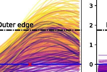
Journal of Vision (2021) 21(8):25, 1–23        Tuhkanen, Pekkanen, Wilkie, & Lappi                                         2

         on and track fixed “waypoints” that may (or may                    a waypoint ahead, in the current direction of travel
         not) be specified by some visible marker. Recent                   at regular intervals of time/space. But with repeated
         evidence has demonstrated that the gaze behaviors                  connected bends that are all equally long, the likelihood
         produced when steering along a path defined using                  of a change in direction (i.e., from a leftward bend to
         only a series of marked waypoints are comparable                   a rightward bend or vice versa when steering through
         to those generated when steering along a winding                   a repeating series of S-bends) increases the deeper
         road (Tuhkanen et al., 2019). Furthermore, when                    one has traveled into each bend. Despite the previous
         steering via visible waypoints, a regular gaze pattern             research that highlights tight coupling between gaze
         akin to “optokinetic pursuit” occurred: looking to                 and steering behaviors, there are a number of questions
         the next waypoint (∼2 s ahead), tracking this point                for which we still do not have clear answers: Can drivers
         with a pursuit eye movement (for ∼0.5 s) before                    produce saccades that reliably predict future waypoint
         generating a further “switch” saccade to look at the               locations even when the bend changes, direction? Will
         next waypoint in the sequence. Crucially, when the                 anticipatory gaze behaviors change depending on how
         next waypoint in the sequence was not visible, gaze                deep the driver is into each bend? If so, will steering
         behavior followed a very similar pattern, suggesting               trajectories reflect gaze changes, or is it the case that
         that much of the gaze–pursuit–switch pattern was                   predictive gaze behaviors start to become decoupled
         internally driven, rather than being solely driven by              from steering control?
         the external visual stimulus. The nature of the internal              A strong focus of (Tuhkanen et al., 2019) was
         driver of visual guidance will be further examined in              comparing gaze patterns between winding roads
         this article: Specifically, can visual sampling behavior be        (demarcated by road lines) and paths specified only
         understood as a simple repeating “motor program,” or               by waypoints. The structure of the scenes used meant
         does it actually reflect genuinely predictive information          that bends were quite long, and advance notice was
         processing? Answers to this fundamental question will              given of changes in bend direction from visual feedback
         lead to a better understanding of locomotor control,               before each inflection point. The scene structure limited
         particularly the ability of humans to drive vehicles at            further analysis of what form of prior information
         speed.                                                             may have been stored to aid predictions about the
                                                                            future path. In the present design, the bends used were
                                                                            shorter and the placement of the waypoints purposely
         Aims of this study                                                 created situations where it was sometimes impossible
                                                                            to anticipate upcoming changes in direction from visual
             In a previous study, we presented participants with            feedback alone. As such, the present experimental design
         a path specified by waypoints embedded in rich optic               should elicit one of the following possible behaviors:
         flow (Tuhkanen et al., 2019). Gaze spontaneously
         tracked these waypoints during the approach, with                 (A) Participants look only at visible waypoints (though
         saccades being generated toward the next waypoint                     this behavior is not expected since this was not
         location further in the distance in an anticipatory                   observed previously by Tuhkanen et al. (2019).
         manner (i.e., even when the next waypoint failed to               (B) Participants look ahead to the predicted location
         appear in the expected location, participants made                    of the “missing waypoint” based on the previous
         saccades to the approximate location of the “missing                  waypoint location (i.e., prediction of the future path
         waypoint”). Through a careful analysis of the saccade                 is limited to constant-curvature bends).
         characteristics, many online/heuristic strategies could           (C) Participants look ahead to the predicted location
         be ruled out (i.e., gaze patterns were found not to be                of the “missing waypoint” based on some
         consistent with simple bottom-up visual transitions or                representation of the S-bend structure as well as an
         generating saccades toward salient locations). These                  internal estimate of current (spatial or temporal)
         analyses suggested that for this phase of the locomotor               position.
         task at least (traveling on a constant radius bend),
         the anticipation of future waypoints appeared to be
         genuinely predictive.
             One question this evidence does not directly answer              Method
         is: What happens when the road curvature is not
         constant but changes in a predictable manner? If the                  Participants drove along a continuous winding course
         observer is driving along a path constructed from a                specified by a series of visible waypoints generated
         repeated series of identical S-bends (with the same                within a fixed-base driving simulator (open source,
         curvature), then the regularity and predictability of              available at https://github.com/samtuhka/webtrajsim/
         the scene may lead to stored representations about                 tree/birch20). The course was displayed visually
         waypoint locations that inform gaze patterns. A coarse             using intermittently appearing waypoints as shown in
         form of representation might lead the driver to predict            Figure 1 (to control the available preview information

Downloaded from jov.arvojournals.org on 10/01/2021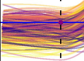
Journal of Vision (2021) 21(8):25, 1–23             Tuhkanen, Pekkanen, Wilkie, & Lappi                                              3

         Figure 1. Stimuli. Top panel: Sample screenshot from a practice trial of the experiment where the track edges were visible. Bottom
         panel: Sample screenshot from a test trial of the experiment where the track edges were invisible. The track was specified by
         gray/white circular waypoints that were presented 80% of the time (VIS condition) at 1-s intervals and 20% of the time (MISS
         condition) at 2-s intervals with a virtual “missing waypoint” in between two visible ones. The waypoints always appeared at a 2-s time
         headway (TH) from the driver. The five square markers were fixed on the screen and used to determine a homography from the eye
         tracker’s camera image to the screen.

         of the road ahead). Participants were asked to stay on                  the main differences being the waypoint placement
         the “track”—track edges were only indicated visually                    and design in order to better gauge how participants
         during the practice trial; during the experimental                      anticipate and react to the change in direction as they
         trials, an auditory tone indicated that the driver had                  near and pass the inflection point of an S-bend. In
         deviated more than 1.75 m from the (invisible) track                    the previous experiment (Tuhkanen et al., 2019), the
         center. Steering was controlled using a Logitech G920                   bends were longer, meaning there were less data from
         Driving Force (Logitech, Fremont, CA) gaming wheel                      inflection points, and the change in direction was easier
         (auto-centering was on but otherwise there was no                       for participants to discern as there was always at least
         force-feedback). The simulator used a raycast vehicle                   one visible waypoint before the inflection point from
         model (as implemented in the Cannon.js JavaSript                        which it was possible to determine whether the bend
         physics library) to simulate vehicle physics. Locomotor                 was about to change direction.
         speed was kept constant at 10.5 m/s (no gears, throttle,
         or brakes were used). Eye movements were recorded
         with a head-mounted eye tracker. The simulator ran                      Participants
         at 60 Hz and was displayed on a 55–in. LG 55UF85
         monitor. The experimental design was similar to the                       A sample of 16 participants (8 female, 8 male, mean
         Experiment 2 described in Tuhkanen et al. (2019), with                  age = 30, SD = 7, range = 22–47) was recruited through

Downloaded from jov.arvojournals.org on 10/01/2021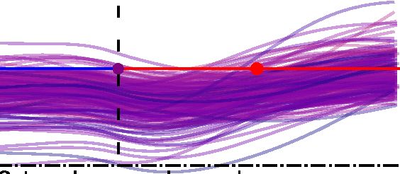
Journal of Vision (2021) 21(8):25, 1–23      Tuhkanen, Pekkanen, Wilkie, & Lappi                                             4

         University of Helsinki mailing lists. All participants           segmentation – (i.e., the gaze data are modeled as
         had a minimum of 20,000 km of driving experience                 successive linear segments). The accompanying hidden
         and reported normal or corrected vision. After the               Markov model (NSLR-HMM) classifies the different
         experiment, the participants were rewarded with three            segments into saccades, fixations, smooth pursuits, and
         exercise and cultural vouchers worth €15 in total for            postsaccadic oscillations. In our experience, the saccade
         participation.                                                   identification is the most reliable component and was
                                                                          the only one used in our analyses.

         Eye tracker
                                                                          Design and stimuli
            The eye movements of the participants were recorded
         with Pupil Core (Pupil Labs UG haftungsbeschränkt,                  The participants drove through a track consisting
         Berlin, Germany) eye tracker. Binocular cameras                  of 120◦ arc curves (radius = 50 m) alternating to left
         recorded at 60 Hz at 640 × 480 resolution while one              and right (see Figure 2). A single trial consisted of 16
         forward-camera recorded the scene at 30 Hz at 1,280 ×            constant-radius curves and took approximately 160 s
         720 resolution. The open-source Pupil Capture software           to complete. The track width was 3.5 m, though the
         (https://github.com/pupil-labs/pupil) was used to record         track edges were only visible in the first practice trial.
         and calibrate the eye tracker. No head or chin rest was          If the participant drove off the track (absolute track
         used, and participants were given no gaze instructions           position > 1.75 m from the centerline), the simulator
         outside the calibration.                                         started playing a constant “beeping” sound until the
            The eye tracker was calibrated at the beginning of            participant returned to the track.
         the experiment and between every few trials (generally,             The participants completed three practice trials at
         every two trials at the experimenter’s determination).           the start of the experiment (practice trials were shorter
         The “2D pipeline” of Pupil Capture was used for                  than test trials and lasted for approximately 50 s). In
         calibration (i.e., a polynomial fit between the center           the first practice trial, the edge lines of the track were
         positions of the pupil and the detected marker positions         visible to introduce the participants to the track and get
         was used to estimate gaze position). The gaze signals            familiar with the dynamics of the virtual car. A sample
         from both eye cameras were averaged together to a                of the first practice trial can be seen in Movie 1. In the
         cyclopean gaze signal. In Tuhkanen et al. (2019), we             second practice trial, the track could only be discerned
         estimated the mean calibration accuracy when using a             through the waypoints, but unlike in the test trials, there
         nearly identical procedure to be approximately 1 degree.         were no missing waypoints. See Movie 2 for a sample
         Mean accuracy here refers to the mean angular distance           trial of the second practice. The third practice trial
         between the calibration marker centers and gaze as               was identical to the test trials. The actual experiment
         measured at the end of the trials in Tuhkanen et al.             consisted of 10 test trials. See Movies 3–4 for sample
         (2019).                                                          test trials. In addition, there were six randomly placed
                                                                          control trials where there were no missing waypoints,
                                                                          but these were ultimately not utilized in the analysis.
         Gaze signal segmentation and classification                          The speed of the virtual vehicle was kept constant
                                                                          at approximately 10.5 m/s, corresponding to a 12 ◦ /s
            The gaze signal of the participants was mapped to the         yaw rate during constant-curvature cornering. The
         coordinates of the screen by determining a homography            virtual camera was at the height of approximately 1.2 m
         from the camera coordinates with the aid of five square          from the ground. The ground had a solid gray texture
         optical markers (see Figure 1). See Movie 4 for a sample         (producing zero optic flow)—this was to keep the exper-
         on what the resulting transformation from the eye                imental design as similar as possible to Tuhkanen et al.
         tracker’s forward camera to screen coordinates looks             (2019) and to ensure that the waypoints were the only vi-
         like. The pixel coordinates were then transformed to             sual cues of the driver’s position. In test trials, the track
         (a linear approximation of) angular coordinates. The             could visually be discerned only through waypoints
         horizontal field of view (FoV) rendered was 70◦ , with           (in addition to the apparent movement of waypoints,
         the fixed observer viewing distance (0.85 m) matched to          vehicle roll provided another self-motion cue).
         this rendered FoV. All gaze points were included in the             The rendered waypoints were 0.7 m radius
         data with no additional filtering. Saccade detection and         circles/“blobs” with a linearly fading white texture
         all analyses use the gaze-on-screen position signal.             (see Figure 1). The waypoints were not visible at all
            The gaze signal was classified with the naive                 distances but rather appeared when they were at a 2-s
         segmented linear regression (NSLR) algorithm                     time headway (TH, as defined by a point ahead along
         (Pekkanen & Lappi, 2017) into individual saccades,               the centerline of the track from the driver at the fixed
         fixations, and smooth-pursuit segments. The                      locomotor speed). The waypoints were normally (VIS
         algorithm approximates a maximum likelihood linear               condition) equally placed at a distance of approximately

Downloaded from jov.arvojournals.org on 10/01/2021
Journal of Vision (2021) 21(8):25, 1–23 Tuhkanen, Pekkanen, Wilkie, & Lappi 5
Figure 2. Bird’s-eye view of the geometry of the track and the indexing convention of the curve segments. The participants drove
through 50-m radius curves alternating to left and right. Each curve consisted of 10 (visible or missing) waypoints and segments. Top
left panel: Indexing of the curve segments (CURV-SEG) used for analysis purposes to divide the data. CURV-SEG = 0 starts when the
driver passes through the inflection point between two curves. Note only waypoints, not track edges, were visible during
experimental trials Top right panel: WP placement during CURV-SEG = 9—the final CURV-SEG before the inflection point. The driver
(black rectangle) is set at the beginning of a CURV-SEG while the dots indicate the positions of WPconst (blue), WPprev (purple), and
WPalt (red). The red trajectory indicates the true centerline following the inflection point and WPalt the location of the most distant
WP while the dashed blue trajectory and WPconst (virtual) indicate where the path would continue assuming a constant-curvature
path. Top right panel: WP placement during CURV-SEG = 5. The constant-curvature assumption is correct here, and always when
CURV-SEG = 9.
10.5 m from one another, corresponding to 1 s in travel (referred to from here on as CURV-SEG) with the index
time. However, as a manipulation, approximately 20% changing when the furthest WP changes. Right and
of the waypoints did not appear (MISS condition). left turning curves were considered equivalent, with
These “missing waypoints” were always separated from left-turning curves being mirrored for all analyses.
one another by at least three visible waypoints. When CURV-SEG refers to the sections of the track where
comparing the VIS condition to the MISS condition, the furthest waypoint, whether visible or not, is at 1
to make the conditions as comparable as possible with s < TH ≤ 2 s. The driver passes the inflection point
the only exception being the visibility of the furthest between two curves when they enter CURV-SEG =
waypoint (WP), only segments where the last three 0. At CURV-SEG = 8, the most distant WP is at the
waypoints had been visible were included in the analysis inflection point. The most distant WP at CURV-SEG
of the VIS condition. = 9 is the first waypoint in the opposite direction to
In total, each constant-radius curve consisted of the current curve. In other words, it is the first of the
10 waypoints (see Figure 2). As the waypoints were waypoints that are located on the upcoming curve (the
located at the same angular positions in every curve, we first waypoint after the inflection point). Even though
discretized and indexed each curve into 10 segments they were not visible, missing waypoints in the MISS
Downloaded from jov.arvojournals.org on 10/01/2021Journal of Vision (2021) 21(8):25, 1–23 Tuhkanen, Pekkanen, Wilkie, & Lappi 6
Figure 3. A sample gaze and waypoint time series from a single participant. Top panel: Horizontal screen positions in respect to
CURV-SEG. Gaze tracking is depicted as green points while the yellow lines indicate the saccades that were derived using the
NSLR-HMM algorithm. Blue lines indicate the location of WPconst , red the location of WPalt , and purple the location of WPprev . Solid
lines indicate the WP in question is visible, whereas dashed lines indicate that it is missing/virtual. WPconst is always visible except
when CURV-SEG = 9 and the MISS condition does not apply. WPalt is only visible when CURV-SEG = 9 and the VIS condition applies.
WPprev is visible when the previous WPconst (CURV-SEG = 9) or WPalt (CURV-SEG = 9) is visible. In the sample times series, the
sienna-colored sections highlight the MISS manipulations and the cyan-colored sections highlight the part of the VIS condition that
was included in the data analysis (i.e., when the furthest WP is visible and the last three WPs have all been visible). Bottom panel:
Same as top panel but with vertical positions depicted instead.
condition were treated the same way in the indexing waypoint that had appeared at TH 2 s at the start of the
scheme. previous CURV-SEG).
Waypoints were further classified as WPconst or A sample time series of the screen positions of the
WPalt on the basis of whether they were on the WPs and the gaze signal can be seen in Figure 3.
constant-radius curve or not. When CURV-SEG ≤ 8,
WPconst is the most distant WP (visible or missing). At
CURV-SEG = 9, however, WPalt is the most distant WP Steering and overall performance
(visible or missing).
We still determined a WPalt for every CURV-SEG— We did a cursory analysis of steering in the VIS and
these served as virtual waypoints “where the next MISS conditions in respect to CURV-SEG. This was
waypoint should appear if the previous waypoint done in order to examine whether the conditions were
was in fact an inflection point.” This was to probe comparable to one another and whether the different
whether participants would direct gaze according to CURV-SEGS were comparable to one another. The
this “alternative hypothesis,” especially in the MISS reasoning was to minimize the possibility that any
condition (see Figure 2). Similarly, we determined a differences in gaze behavior between the conditions
virtual WPconst for CURV-SEG = 9 (“where the next and with respect to CURV-SEG could not simply be
waypoint should appear if the last waypoint was in explained differences in steering.
fact not an inflection point”). We use the convention Mean track position (i.e., distance from centerline)
WPprev to refer to the waypoint at 0 < TH ≤ 1 (i.e., the and mean steering wheel angle in the different
Downloaded from jov.arvojournals.org on 10/01/2021Journal of Vision (2021) 21(8):25, 1–23 Tuhkanen, Pekkanen, Wilkie, & Lappi 7
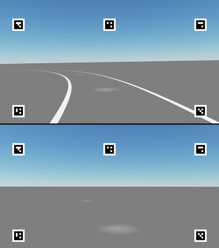
Figure 4. Sample frame from Movie 5. Top panel: The gaze density distribution (across all participants and trials) in the MISS condition
in CURV-SEG = 1, at the time point when the time headway to the furthest (but missing) waypoint is 1.42 s. The blue cross indicates
the position of the (missing) WPconst , the red cross the virtual WPalt , and the purple dot WPprev (i.e., the last waypoint that was
actually observed). All the coordinates have been normalized with respect to the position of WPconst , and the relative positions
between WPalt and WPconst should be effectively constant across trials. (Due to projection geometry, it changes with time headway.)
The full movie shows the gaze distribution developing across each CURV-SEG. All left-turning segments of the data have been
mirrored. Middle left panel: The marginal gaze distributions for the x-axis in the VIS and MISS conditions. Middle right panel:
Bird’s-eye view of the track. The black dotted line indicates the (invisible) centerline of the track and the solid blue line the extent of
the CURV-SEG 01. The blue dot indicates the location of WPconst , the red dot the location of WPalt , and the purple dot the location of
WPprev . The gray dot indicates the position of the driver within the CURV-SEG. Bottom panel: The comparable gaze density
distribution as in the top panel but in the VIS condition where the waypoint at TH = 1.42 s is, in fact, visible (having appeared at TH =
2.0 s). The blue dot indicates the location of the visible WPconst and the red cross the WPalt .
conditions are shown in Figure A1. Steering behavior waypoint (each missing waypoint was always followed
during CURV-SEG = 0 (where there is a transition to by a minimum of three visible waypoints).
change bend direction) differs from the other segments
where steering remains relatively stable. To avoid
confounds related to differential steering for VIS and
MISS conditions, CURV-SEG = 0 was excluded from Results
further analyses.
In terms of overall steering performance, the The general pattern of the participant gaze
participants drove off the track relatively rarely. An distribution at each point in time and each
auditory tone was sounded to give feedback to the CURV-SEG is visualized in Movie 5 (https:
participant that they had left the track. The median //doi.org/10.6084/m9.figshare.14828928, see Figure
participant spent approximately 1% of the total runtime 4 for a sample frame). As in Tuhkanen et al. (2019),
off the track (range = 0.1%–4.0%). Approximately participants shift their gaze from the previous
99% of the total off-track time happened during the waypoint to both the visible and missing waypoint
VIS condition—presumably following a recent missing locations ahead. Unlike in Tuhkanen et al. (2019),
Downloaded from jov.arvojournals.org on 10/01/2021Journal of Vision (2021) 21(8):25, 1–23 Tuhkanen, Pekkanen, Wilkie, & Lappi 8
however, in the case of the MISS condition, the = 0 was excluded from the analysis due to incomparable
gaze distribution appears to horizontally spread out steering behavior and because it might still be ambigu-
more as CURV-SEG increases; this possibly reflects ous to the driver whether the inflection of the curve has
increased uncertainty over the location of the future in fact occurred (i.e., whether target path curvature has
path/waypoint and whether it continues along the changed from right-hand to left-hand or vice versa).
current constant-curvature path. To investigate the Mean gaze offsets can be seen in Figure 5 in regard
robustness of this effect and its implications, three to both the MISS and VIS conditions. Participant-wise
main analyses were performed followed by a report on median offsets can be seen in Figure A2. For most
participant strategies. First, we investigated whether participants, the median offset appears to increase as
the horizontal shift in gaze was significant within CURV-SEG increases. To assess this quantitatively,
participants by looking at horizontal gaze offset from Spearman’s rank correlation coefficient was used to
a reference point midway between WPconst and WPalt . estimate the correlation between CURV-SEG and the
Second, we investigated whether the effect persisted median offsets.
when restricting the analysis to examine the saccade After a Fisher’s z transformation, we derived a
landing points. Third, we investigated whether the (retransformed) mean correlation coefficient of 0.67
anticipatory (or seemingly anticipatory) gaze fixations for the MISS condition, with all but one participant
in the vicinity of WPalt correlated with changes in having a positive correlation. The Fisher-transformed
steering. Finally, we discuss the survey of participant correlations were significantly different from zero
strategies. (one-sample t test, p = 0.0002), indicating that the
participants’ gaze drifted more toward the direction
of WPalt the further along a constant-radius curve the
Gaze offset participants were.
If CURV-SEG = 9 is excluded from the data, the
If gaze and steering control employ purely online mean Spearman’s rho is 0.62 with all but one participant
mechanisms (i.e., mechanisms driven by directly having a positive correlation (one-sample t test to test
available external stimuli), there is little apparent reason difference from zero, p = 0.0002). Conversely, in the
to expect gaze behavior to change as a function of how VIS condition when CURV-SEG = 9 is excluded, the
far along a constant-radius curve participants have mean Spearman’s rho is 0.25, with 10 participants
traveled (i.e., similar behavior for CURV-SEG = 1 and having a positive correlation (dependent t test to test
CURV-SEG = 9), especially since the visual scene is very difference from the MISS condition, p = 0.02) —that is,
similar. In contrast, predictive strategies (whether truly with this exclusion, participants on average had a lower
model based or not) should lead to greater uncertainty Spearman’s rho in the VIS condition than in the MISS
about whether future WPs will continue to fall along condition.
the same constant-radius arc as CURV-SEG increases.
If this uncertainty is also reflected in gaze behavior, you
should see more gaze polling at the vicinity of WPalt Saccade landing point classification
and/or hedging somewhere between WPalt and WPconst .
(Although if the predictive ability were perfect, the The results of the offset gaze analysis described in
change in behavior from WPconst to WPalt might only the previous section could, in principle, be explained
happen at CURV-SEG = 9, when the waypoint actually by a decrease in generating saccades toward WPconst
appears, or fails to appear, at the WPalt location.) without a concomitant increase in looking toward
To investigate this, we looked at how and if WPalt . Another way to investigate the underlying
participants’ median horizontal gaze position (in the representation used by participants is to see whether
region horizontally spanning from WPconst to WPalt ) more saccades target WPalt in the MISS condition the
would shift as a function of CURV-SEG. For each deeper into each constant-radius bend the participant
participant and each CURV-SEG, we determined a has traveled (i.e., as CURV-SEG increases). The
median horizontal gaze offset from the horizontal motivation of this investigation was to determine
middle point between WPconst and WPalt —positive whether the participants would actively poll the
values indicate the gaze was closer to WPalt than WPconst . alternate waypoint location (i.e., toward a predicted
Only the last frame of each CURV-SEG was included upcoming change in bend direction) the deeper they
(i.e., the moments in time when the appearance of the were into the bend.
next WP was most imminent). This exclusion was done In addition to using WPconst , WPalt , and WPprev for
to filter out gaze points that may have still been located the saccade classification analysis, a MID classification
in the vicinity of WPprev . As can be seen in Movie 4, for was also created. The location of MID was determined
the last frames of a CURV-SEG, the participant gaze as the arithmetic mean of the screen positions of
is vertically situated mostly at the height (screen y coor- WPprev , WPalt , and WPconst . The purpose of this
dinates) of WPconst and WPalt . In addition, CURV-SEG gaze category was to help classify gaze behavior if
Downloaded from jov.arvojournals.org on 10/01/2021Journal of Vision (2021) 21(8):25, 1–23 Tuhkanen, Pekkanen, Wilkie, & Lappi 9
Figure 5. Left panel: The grand mean horizontal gaze offsets in the VIS (solid green line) and MISS (dashed green line) conditions. The
offsets have been determined as the angular offset from the reference point in the middle between the WPconst and WPalt . Positive
values indicate that the participants’ gaze is on average horizontally closer to WPalt than WPconst . The grand mean was determined by
calculating the mean from participant-wise median offsets. The error bars display the 95% CIs. In the VIS condition, the mean gaze
position stays uniformly at the approximate location of WPconst (–6 degrees) when CURV-SEG ≤ 8 and shifts to the approximate
position of WPalt (6 degrees) at CURV-SEG = 9. In contrast, in the MISS condition, the mean gaze position gradually shifts toward
WPalt (though still remains closer to WPconst than WPalt ) as CURV-SEG increases. Right panel: The mean ratio of saccades classified as
landing toward WPalt in the VIS and MISS conditions in respect to CURV-SEG. Before averaging the participants, each saccade was
classified in respect to which waypoint (WPalt , WPconst , WPprev , or MID) was nearest to the saccade landing point, and the proportion
of saccades landing toward WPalt was determined for each participant (which were then averaged). In the VIS condition, almost none
of the saccades land toward WPalt except when CURV-SEG = 9 when almost all do (this is expected as in the VIS condition,
WPalt is visible when CURV-SEG = 9, whereas WPconst is at all other times). In the MISS condition, the ratio gradually increases as
CURV-SEG increases, possibly indicating greater uncertainty on whether the track will continue along the same constant-radius arc.
participants do not (clearly) target any of the waypoint t test, p = 0.0003) indicating that the participants’
locations and instead place their gaze somewhere saccades landed more often in the vicinity of WPalt as
between the alternatives locations (potentially in order CURV-SEG increased (and the inflection point of the
to be able to detect WPs in either alternative location in bend was approached).
the visual periphery). If CURV-SEG = 9 is excluded from the data, the
This analysis determined the distance (in screen mean Spearman’s rho is 0.57 with all but one participant
coordinates) between each saccade landing point to having a positive correlation (one-sample t test to test
WPalt , WPconst , MID, and WPprev . Each saccade landing difference from zero, p = 0.0003). Conversely, in the VIS
point was then classified (as one of the three WPs or condition when CURV-SEG = 9 is excluded, the mean
MID) depending on which region it was closest to. For Spearman’s rho is −0.24 with only four participants
each participant, the ratio of saccades in the WPalt with having a positive correlation (dependent t test to test
respect to CURV-SEG was calculated (CURV-SEG = difference from the MISS condition, p = 0.0001) —that
0 was excluded as described in the previous analysis). is, with this exclusion, participants on average had a
The ratios with respect to CURV-SEG are visualized in lower Spearman’s rho in the VIS condition than in the
Figure 5. Participant-wise ratios can be seen in Figure MISS condition.
A3. As in the offset analysis, Spearman’ r was used to
measure the correlation between CURV-SEG and the
ratio of WPalt classified saccades. The effect of gaze position on steering
After a Fisher’s z transformation, we derived a
(retransformed) mean correlation coefficient of 0.63 for We have observed that gazing behavior shifts
the MISS condition with all but one participant having toward WPalt in the MISS condition as CURV-SEG
a positive correlation. The z-transformed correlations increases. To see if this at least seemingly predictive
were significantly different from zero (one-sample gaze behavior has any effect on steering, we investigated
Downloaded from jov.arvojournals.org on 10/01/2021Journal of Vision (2021) 21(8):25, 1–23 Tuhkanen, Pekkanen, Wilkie, & Lappi 10
Figure 6. Top left panel: Participant trajectories in regards to track positions from −1 s before the inflection point to +2 s after the
inflection point when WPalt during CURV-SEG = 9 in the MISS condition. The individual trajectories have been colored by the
horizontal gaze offset at the end of CURV-SEG = 9. Positive gaze offset indicates the gaze was closer to WPalt than WPconst and
negative that gaze was closer to WPconst . When gaze offset is more toward WPconst , the participants appear to steer closer toward the
outer edge as opposed to steering closer toward the inner edge when gaze is closer to WPalt . Top right panel: Comparable to the top
left panel but from the VIS condition. Only trajectories where WPs are visible during the whole –1- to +2-s duration (i.e., the two
following CURV-SEGs are also part of the VIS condition). Lower left panel: Participant trajectories in regards to x,y coordinates from
–1 s before the inflection point to +2 s after the inflection point when the furthest waypoint during CURV-SEG = 9 was missing. Note
that the track edges and centerline were not visible (leaving the track caused a warning beep to sound). Lower right panel:
Comparable to the lower left panel but from the VIS condition. Only trajectories where WPs are visible during the whole –1- to +2-s
duration (i.e., the two following CURV-SEGs are also part of the VIS condition).
the correlation between gaze position near the inflection Fisher-transformed participant correlations) of –0.70.
point (e.g., at the end of CURG-SEG = 9) at each run The full trajectories in regards to gaze offset and both
and what their future trajectory was. track position and x,y-coordinates can be seen in Figure
More precisely, we calculated the horizontal gaze 6. A scatterplot of the calculated mean track positions
offset from the final frame of CURV-SEG = 9 and then is visualized in Figure 7; otherwise, identical analysis
calculated the mean track position from the following but with steering wheel deviation as the dependent
2 s (i.e., CURV-SEG = 1 and CURV-SEG = 2) after variable instead of mean track position is displayed in
the inflection point. With positive track positions Figure A6.
indicating a position that was more toward the outer
edge of the track and positive offset indicating a gaze
position closer to WPalt than WPconst , every participant Participant strategies
had a negative Pearson’s correlation coefficient between
gaze offset and track position (t test to test difference At the end of the experiment, each participant
from 0, p < 0.0001) with a mean correlation (from answered a quick survey that checked whether they
Downloaded from jov.arvojournals.org on 10/01/2021Journal of Vision (2021) 21(8):25, 1–23 Tuhkanen, Pekkanen, Wilkie, & Lappi 11
Figure 7. Scatterplot of track position as a function of horizontal gaze offset at the end of CURV-SEG = 9. Small gray dots indicate
individual runs from all participants when WPalt was missing during CURV-SEG = 9. Mean track positions have been calculated from
the 2 s following the inflection point. Colored lines indicate the slopes of participant-wise linear OLS fits (diamond the location of the
participant mean)—line width is proportional to participant’s standard deviation of gaze offset (total width = 0.5 * SD). Participants 1,
6, 13, and 16 reported to have counted the WPs (see participant strategies) and are marked with a black center within the diamond
marker. The pooled fit (dashed black line) has been calculated from the data of all participants (note that the r is different from the
mean participant r of –0.7). All participants have a negative correlation, and the Participant means except for Participant 15 appear to
mostly follow the general trend of higher gaze offset being associated with track position away from the outer edge (track position =
1.75) and toward the inner edge (track position = –1.75).
had used any specific strategies to predict when the anticipatory gaze behavior would occur when there
direction of the track changed. Out of 16 participants, were predictable—but visually withheld—changes in
4 (Participants 1, 6, 13, 16) mentioned that they had (at path direction. Participants steered through a series
least at some point during the experiment) attempted of S-bends (with an “inflection” point at the end
to count waypoints to predict when the direction of the of each bend), and the analyses confirmed previous
curve would change. However, when asked to estimate findings: Gaze was directed to the predictable location
how many waypoint locations (i.e., the sum of visible of future waypoints, even when that waypoint was not
and missing waypoints) there were there on a single visible.
constant radius curve, 6 participants (Participants 1, 6, Because of the alternating direction of bends, the
10, 13, 14, 16 in the participant-wise figures) were able location of the next waypoint varied according to how
to answer correctly. “deep” into each bend the driver had traveled when the
waypoint was withheld. The first waypoint after bend
inflection appeared in a markedly different location in
the visual field compared to the preceding waypoints.
Discussion If participants could determine how deep into each
bend they had traveled (either through a spatial or
Tuhkanen et al. (2019) observed that people shift temporal estimate or some combination thereof), they
their gaze toward the future path (marked by a series of should be able to anticipate the bend change and shift
waypoints) even when the visual information specifying gaze accordingly to predict the future path. Due to
the future path was withheld. These anticipatory gaze the sparse visual environment, any estimate should be
shifts toward the future waypoint location in the uncertain (probabilistic), and so the gaze sampling from
world took into account variation in road position the “alternative” waypoint location should increase as
and heading, indicating that gaze behavior was the inflection point was approached.
genuinely predictive (rather than being explained by a Our analysis confirmed that gaze behavior did
low-level motor response). However, these findings were indeed change depending on how deep into each
potentially limited by the highly regular constant-radius bend participants traveled. When visual cues to the
paths that were used since most waypoints were future path were absent, participants’ gaze shifted
positioned in very similar parts of the visual field. In more toward the alternative waypoint location the
the present study, we investigated whether the same further they had traveled along the current bend. When
Downloaded from jov.arvojournals.org on 10/01/2021Journal of Vision (2021) 21(8):25, 1–23 Tuhkanen, Pekkanen, Wilkie, & Lappi 12
waypoints along the future path were all visible, no Some participants appear to explicitly estimate how
such shift in gaze behavior was apparent (until the many waypoint locations each bend consisted of and
visible waypoint actually appeared at the alternative kept a count of them to keep track of their location.
bend location). The observed gaze behavior provides With this cognitive strategy, a choice could then be
evidence for greater visual anticipation than previously made between producing a saccade “in the direction
reported: both reflecting upcoming directional changes of rotation” or “in the opposite direction of rotation.”
in steering, as well as increasing uncertainty about the This could have been based on the display frame of
likely direction of the future path. reference or with reference to the actual future path
It might be tempting to discount these changes in the world (“after x number of waypoint locations,
in gaze behavior as being relatively “cheap”: Eye the bend curvature will change”). It should be noted
movements are low effort to produce and are low cost that this approach is not trivial since it requires the
(in both time and energy) to change again in the future. participants to count missing WPs as well as visible
By this logic, wider dispersal of gaze could simply be ones. While four participants (P1, P6, P13 and P16)
considered as some general search strategy when there is explicitly reported attempting to count path features
uncertainty without a clear relationship to the planned (waypoints/waypoint locations/curve segments—the
trajectory of the future path. But previous research exact features could not be distinguished based on
has demonstrated that gaze and steering behaviors are the verbal reports), others may have done so without
tightly coupled (Land & Lee, 1994; Wilkie & Wann, disclosing or explicitly realizing it. Regardless of
2003b; Chattington et al., 2007; Robertshaw & Wilkie, whether the use of this cognitive heuristic would qualify
2008; Kountouriotis et al., 2012) and, theoretically, may as a “genuine” representation of the path geometry
be derived from a common underlying representation or not, it is certainly not a pure online strategy.
(Land & Furneaux, 1997; Lappi & Mole, 2018; cf. also And, for all the flaws of self-report methods, such
Tatler & Land, 2011). So, if gaze shifts were genuinely an explicit strategy should have been straightforward
predictive of the expected path/planned trajectory, we for participants to report. Actually, a wide variety of
should also observe shifts in steering to accompany strategies/approaches were reported, most of which
the gaze shifts elicited when the bend inflection point were not straightforward to interpret (i.e., they don’t
was approached. Correlational analyses confirmed that simply map onto a counting waypoints rule), suggesting
steering did indeed shift in the direction of gaze (Figure they were largely implicit. The lack of a single approach
7), as would be expected if prediction was being used itself may be evidence that a form of model-based
to direct gaze and inform steering control (Figure 6). control was invoked since online control strategies
While it is not possible to determine the direction(s) should be highly consistent and (stereotypically at
of causality between gaze and steering using these least) rely upon very few perceptually available signals.
correlations, the directional links between gaze and Alternatively, it could simply highlight a dissociation
steering have been investigated in previous experiments between the participants’ explicit understanding (what
(Wilkie & Wann, 2003b; Kountouriotis et al., 2013; they think they are doing) and their control strategy
Mole et al., 2016). (what they are actually doing) that has been observed
We find it very difficult to explain the observed previously (Mole et al., 2018).
behaviors without recourse to some kind of internal Regardless of the exact strategies used, it is also
representation of the future path. There appears to apparent that participant performance was not perfectly
be no pure online strategy or even a stored (ballistic) accurate. A perfectly precise prediction should lead
motor program that could produce the observed results. to identical gaze behavior irrespective of whether the
While relying upon an internal representation might waypoint was visible or not (i.e., minimal gaze fixations
invoke the idea of a “high-fidelity world model,” it is toward the alternative waypoint except at the bend
also possible that a more or less “weak representation” inflection point). Instead, as participants traveled more
could suffice (Zhao & Warren, 2015). The question deeply into each bend, we observed a gradual increase
here becomes whether gaze shifts toward the alternative in sampling from the region around the alternative
waypoint were supported by a constantly updated waypoint; the positive correlation between alternative
(dynamic) estimate of some features of the path waypoint sampling and curve segments persisted even
geometry, and where on the path they were currently if the last segment before the inflection point was
located, or by some cognitive heuristic and/or (static) excluded from analysis (this did not happen in the
“spatial memory.” The participants might, for example, visible condition). This pattern might be explained by a
have been estimating time or distance or kept count of gradual increase in uncertainty over whether the bend
the waypoints in each curve. is about to change direction the further/longer one has
Further computational modeling and experimental traveled along the current constant-radius curve.
efforts should be made to tease apart these alternatives. Consistent with the individual differences in
But within our data, it does seem that there were self-reported strategies, it was also apparent that
individual differences in the approach to the task. the gaze behaviors adopted by participants were not
Downloaded from jov.arvojournals.org on 10/01/2021Journal of Vision (2021) 21(8):25, 1–23 Tuhkanen, Pekkanen, Wilkie, & Lappi 13
entirely uniform. When looking at the participant-wise experiments complemented with formal modeling. In
figures (Figures A2 and A3), it is clear that the the present study, we demonstrate that when steering
amount of anticipatory gaze behavior varied between through a series of repeating S-bends, participants
participants, and the gradual increase in looking anticipate changes in track curvature with their gaze,
toward the alternative waypoint was not apparent for even when visual cues of changes are withheld. This
all participants. For example, Participant 15 frequently anticipation reflected the increased uncertainty over the
generated saccades toward the alternative waypoint future path as the inflection point of the S-bend was
but did so throughout the constant-radius curve; approached, strongly suggesting that steering control
Participant 6 displayed almost identical behavior is informed by some form of internal representation.
in the case of missing and visible waypoints (i.e., a Prediction appears to play a critical role when it comes
sudden shift toward the alternative waypoint right to explaining the observed gaze and steering behaviors.
before the infliction point) consistent with having a
Keywords: eye movements, prediction, internal model,
very precise estimate of their position on the bend;
steering control, driving
and among Participants 2, 5, 9, 11, and 12, the
amount of anticipatory gaze behavior relative to the
alternative waypoint was small at best. Regardless, for
all participants, an increase in gaze position toward Acknowledgments
the alternative waypoint before the inflection point
correlated with a track position closer to the inner edge The authors thank Roosa Frantsi for valuable help
(Figure 7) and less variance in steering (Figure A6) after with the data collection.
the inflection point, suggesting that the anticipation of
the alternative waypoint facilitated successful steering ST was supported by the grant UPP-
control. PERFORMANCE 325694 funded by the Academy of
Finland. RMW and JP were supported by the grant
TRANSITION EP/P017517/1 funded by EPSRC, UK.
Conclusions OL was supported by the grant Sense of Space 334192
funded by the Academy of Finland.
There is a long and ongoing theoretical debate
about how an active moving animal anticipates future Commercial relationships: none.
action requirements and adjusts their ongoing behavior Corresponding author: Samuel Tuhkanen.
accordingly. Anticipatory behaviors in humans can Email: samuel.tuhkanen@helsinki.fi.
be observed in almost all skilled-action contexts, be it Address: Cognitive Science, Traffic Research Unit,
the timing of a ball catch or driving along a winding University of Helsinki, Helsinki, Finland.
road at speed. However, successful anticipatory actions
could result from fundamentally different processes:
Explanations for anticipatory behavior range from
model-free control to approaches that base action
choice on internal representations. Model-free control
References
relies upon a controller that is coupled directly to
the information that is available to the organism Bubić, A., Cramon, D., & Schubotz, R. (2010).
and emerges from the animal’s interaction with the Prediction, cognition and the brain. Frontiers in
environment (Zhao & Warren, 2015; Gibson, 1986) Human Neuroscience, 4, 25.
or on motor programs that run their course in a Chattington, M., Wilson, M., Ashford, D., & Marple-
ballistic manner (the environmental information merely Horvat, D. (2007). Eye–steering coordination in
specifies when the motor program is launched and natural driving. Experimental Brain Research,
its parameters). Other forms of control are model 180(1), 1–14.
based, meaning that the organism maintains some Cutting, J. E. (1986). Perception with an eye for motion
kind of structured internal representation about the (Vol. 1). Cambridge, MA: MIT Press.
environment (i.e., a memory structure that contains
Cutting, J. E., Springer, K., Braren, P. A., & Johnson,
more than just a set of stored values of controller
S. H. (1992). Wayfinding on foot from information
parameters; see Zhao & Warren, 2015; Bubić et al.,
in retinal, not optical, flow. Journal of Experimental
2010). If the organism further maintains an internal
Psychology: General, 121(1), 41.
representation of the environment’s dynamics and uses
this to update its model, the representations are said to Gibson, J. J. (1986). The ecological approach to visual
be generative or predictive. perception. New York, NY: Psychology Press.
For the field to progress, it is important that any Grasso, R., Prévost, P., Ivanenko, Y. P., & Berthoz, A.
underlying representations are probed by critical (1998). Eye-head coordination for the steering of
Downloaded from jov.arvojournals.org on 10/01/2021Journal of Vision (2021) 21(8):25, 1–23 Tuhkanen, Pekkanen, Wilkie, & Lappi 14
locomotion in humans: an anticipatory synergy. Mole, C. D., Kountouriotis, G., Billington, J., & Wilkie,
Neuroscience Letters, 253(2), 115–118. R. M. (2016). Optic flow speed modulates guidance
Kountouriotis, G. K., Floyd, R. C., Gardner, P. H., level control: New insights into two-level steering.
Merat, N., & Wilkie, R. M. (2012). The role of Journal of Experimental Psychology: Human
gaze and road edge information during high-speed Perception and Performance, 42(11), 1818–1838.
locomotion. Journal of Experimental Psychology: Pekkanen, J., & Lappi, O. (2017). A new and general
Human Perception and Performance, 38(3), 687–702. approach to signal denoising and eye movement
Kountouriotis, G. K., Shire, K. A., Mole, C. D., classification based on segmented linear regression.
Gardner, P. H., Merat, N., & Wilkie, R. M. Scientific Reports, 7(1), 17726.
(2013). Optic flow asymmetries bias high-speed Raviv, D., & Herman, M. (1991). A new approach
steering along roads. Journal of Vision, 13(10), 23, to vision and control for road following. In
doi:10.1167/13.10.23. Proceedings of the IEEE Workshop on Visual
Land, M. F., & Furneaux, S. (1997). The knowledge Motion (pp. 217–225).
base of the oculomotor system. Philosophical Regan, D., & Gray, R. (2000). Visually guided collision
Transactions of the Royal Society of London, Series avoidance and collision achievement. Trends in
B: Biological Sciences, 352(1358), 1231–1239. Cognitive Sciences, 4, 99–107.
Land, M. F., & Lee, D. N. (1994). Where we look when Robertshaw, K. D., & Wilkie, R. M. (2008). Does gaze
we steer. Nature, 369(6483), 742–744. influence steering around a bend? Journal of Vision,
Lappi, O. (2014). Future path and tangent point models 8(4), 18, doi:10.1167/8.4.18.
in the visual control of locomotion in curve driving. Tatler, B. W., & Land, M. F. (2011). Vision and the
Journal of Vision, 14(12), 21, doi:10.1167/14.12.21. representation of the surroundings in spatial
Lappi, O., & Mole, C. (2018). Visuomotor control, eye memory. Philosophical Transactions of the Royal
movements, and steering: A unified approach for Society B: Biological Sciences, 366(1564), 596–
incorporating feedback, feedforward, and internal 610.
models. Psychological Bulletin, 144(10), 981. Tuhkanen, S., Pekkanen, J., Rinkkala, P., Mole, C.,
Lappi, O., Pekkanen, J., & Itkonen, T. H. (2013). Wilkie, R. M., & Lappi, O. (2019). Humans use
Pursuit eye-movements in curve driving differentiate predictive gaze strategies to target waypoints for
between future path and tangent point models. steering. Scientific Reports, 9(1), 8344.
PLoS One, 8(7), e68326. Vansteenkiste, P., Van Hamme, D., Veelaert, P.,
Lappi, O., Pekkanen, J., Rinkkala, P., Tuhkanen, S., Philippaerts, R., Cardon, G., & Lenoir, M. (2014).
Tuononen, A., & Virtanen, J.-P. (2020). Humans Cycling around a curve: The effect of cycling speed
use optokinetic eye movements to track waypoints on steering and gaze behavior. PLoS One, 9(7),
for steering. Scientific Reports, 10(1), 4175. e102792.
Lee, D. N. (1976). A theory of visual control of braking Wann, J., & Land, M. (2000). Steering with or without
based on information about time-to-collision. the flow: Is the retrieval of heading necessary?
Perception, 5(4), 437–459. Trends in Cognitive Sciences, 4(8), 319–324.
Matthis, J. S., Muller, K. S., Bonnen, K., & Hayhoe, Wilkie, R. M., & Wann, J. P. (2003a). Controlling
M. M. (2021). Retinal optic flow during natural steering and judging heading: Retinal flow, visual
locomotion. bioRxiv. direction, and extraretinal information. Journal of
Experimental Psychology: Human Perception and
Matthis, J. S., Yates, J. L., & Hayhoe, M. M. (2018).
Performance, 363–378.
Gaze and the control of foot placement when
walking in natural terrain. Current Biology, 28(8), Wilkie, R. M., & Wann, J. P. (2003b). Eye-movements
1224–1233. aid the control of locomotion. Journal of Vision,
3(11), 3, doi:10.1167/3.11.3.
Mole, C. D., Jersakova, R., Kountouriotis, G. K.,
Moulin, C. J. A., & Wilkie, R. M. (2018). Zhao, H., & Warren, W. H. (2015). On-line and
Metacognitive judgements of perceptualmotor model-based approaches to the visual control of
steering performance. Quarterly Journal of action. Vision Research, 110, 190–202.
Experimental Psychology, 71(10), 22232234.
Downloaded from jov.arvojournals.org on 10/01/2021You can also read