Very-long-period oscillations in the atmosphere (0-110 km) - Part 2: Latitude-longitude comparisons and trends
←
→
Page content transcription
If your browser does not render page correctly, please read the page content below

Research article
Atmos. Chem. Phys., 23, 3267–3278, 2023
https://doi.org/10.5194/acp-23-3267-2023
© Author(s) 2023. This work is distributed under
the Creative Commons Attribution 4.0 License.

                            Very-long-period oscillations in the
                         atmosphere (0–110 km) – Part 2: Latitude–
                            longitude comparisons and trends
                   Dirk Offermann1 , Christoph Kalicinsky1 , Ralf Koppmann1 , and Johannes Wintel1,2
          1 Institut   für Atmosphären- und Umweltforschung, Bergische Universität Wuppertal, Wuppertal, Germany
                                  2 Elementar Analysensysteme GmbH, Langenselbold, Germany

                                  Correspondence: Dirk Offermann (offerm@uni-wuppertal.de)

                                   Received: 22 September 2022 – Discussion started: 3 November 2022
                           Revised: 13 February 2023 – Accepted: 20 February 2023 – Published: 14 March 2023

       Abstract. Measurements of atmospheric temperatures show a variety of long-term oscillations. These can be
       simulated by computer models and exhibit multi-annual, decadal, and even centennial periods. They extend from
       the ground up to the lower thermosphere. Recent analyses have shown that they exist in the models even if the
       model boundaries are kept constant with respect to influences of the sun, ocean, and greenhouse gases. There-
       fore, these parameters appear not to be responsible for the excitation of these oscillations, i.e. the oscillations
       might be rather self-excited. However, influences of land surface and vegetation changes had not been entirely
       excluded. This is studied in the present analysis. It turns out that such influences might be active in the lowermost
       atmospheric levels.
          Long-term trends of atmospheric parameters such as the temperature are important for the understanding of
       the ongoing climate change. Their study is mostly based on data sets that are 1 to a few decades long. The
       trend values are generally small and so are the amplitudes of the long-period oscillations. It can therefore be
       difficult to disentangle these structures, especially if the interval of trend analysis is comparable to the period of
       the oscillations. If the oscillations are self-excited, there may be a non-anthropogenic contribution to the climate
       change which is difficult to determine. Long-term changes of the cold-point tropopause are analysed here as an
       example.

1   Introduction                                                      oscillations may be difficult to disentangle from the trends.
                                                                      This is especially important if the oscillations are part of
Long-period temperature oscillations have been observed in            the internal variability of the atmosphere. Internal and nat-
atmospheric measurements and – surprisingly – in a very               urally forced variability – for instance, on decadal timescales
similar form in general circulation models (e.g. Meehl et al.,        – is discussed by Deser (2020) and in the IPCC Climate
2013; Deser et al., 2014; Lu et al., 2014; Dai et al., 2015; Di-      Change 2021 report (Eyring et al., 2021).
jkstra et al., 2006; for further references, see Offermann et al.,       The analyses of Offermann et al. (2021) show very-long-
2021). The latter authors have reported decadal to even cen-          period oscillations that appear to be of internal (self-excited)
tennial oscillation periods that not only existed at the surface      origin but whose detailed nature is as yet unknown. There-
but extended from the ground to the lower thermosphere. It            fore, that paper collected a number of characteristic struc-
was shown that they were not excited by the sun, the ocean,           tures which may help to clarify that question. This approach
or greenhouse gases. The amplitudes of these oscillations are         is further followed here by a comparative study of four lo-
not large (i.e. fractions of 1 K). Nevertheless they may be           cations in the Northern and Southern Hemispheres (at 50◦ N
important if long-term trends of temperature are analysed,            vs. 50◦ S, both at 7◦ E, and at 70 and 280◦ E, both at 75◦ N;
as such trends are on this order of magnitude. Hence, these           coordinates are approximate).

Published by Copernicus Publications on behalf of the European Geosciences Union.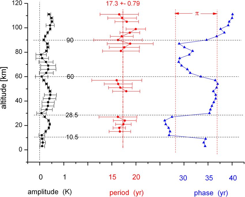
3268                                  D. Offermann et al.: Very long period oscillations in the atmosphere (0–110 km) – Part 2

                                                                       ature. Such trends in the lower and middle atmosphere have
                                                                       been discussed frequently. They are positive or negative, de-
                                                                       pending on altitude. Recent analyses for the troposphere and
                                                                       stratosphere have been presented, for instance, by Steiner et
                                                                       al. (2020), based on numerous measured data. Such analyses
                                                                       generally cover only a few decades. Therefore, the changes
                                                                       are usually small and often comparable to the oscillation am-
                                                                       plitudes mentioned. It can sometimes be difficult to analyse
                                                                       them.
                                                                          Of special interest are temperature changes near the
                                                                       tropopause, as the tropopause is influenced by many pa-
                                                                       rameters and is believed to show a robust “fingerprint” of
                                                                       climate change (Santer et al., 2004; Pisoft et al., 2021).
                                                                       Tropopause trend analyses have been presented several times
                                                                       (e.g. Zhou et al., 2001; Gettelman et al., 2009; Hu and Val-
                                                                       lis, 2019). Long-term changes of tropopause and stratopause
                                                                       altitudes have been analysed by means of measured and
Figure 1. Vertical structures of long-period oscillations near 17.3±   modelled data by Pisoft et al. (2021). They find important
0.8 yr from HAMMONIA temperatures.                                     changes, such as an increase in tropopause height and a con-
                                                                       traction of the stratosphere, which they attribute mainly to
                                                                       long-term increases of greenhouse gases. The temperature
   The long-period oscillations of Offermann et al. (2021)             at the tropopause is frequently studied as the “cold-point
were not excited by influences from the sun, ocean, and                tropopause” (CPT), i.e. the lowest temperature between the
greenhouse gases. Therefore, self-excitation had been con-             troposphere and stratosphere. It is influenced by various at-
sidered as a possibility. However, doubts remained as to a             mospheric parameters and is therefore discussed as a climate
possible excitation by land surface–atmosphere interactions            indicator (Hu and Vallis, 2019; Gettelman et al., 2009).
(see their Sect. 2.2). We therefore compare here locations and            Long-term changes of the CPT are of specific interest.
occasions with very different surface structures. The location         They have been analysed in the tropics several times. Zhou et
50◦ N is in middle of the European land mass. The location             al. (2001) find a negative trend of −0.57 ± 0.06 K per decade
50◦ S is about 15◦ S of the tip of South Africa in the South-          in the time interval 1973–1998. RavindraBabu et al. (2020)
ern Ocean. The polar locations are in northernmost Canada              find a trend of −1.09 K per decade in the time interval 2006–
and Siberia. Concerning land surface–atmosphere interac-               2018. Tegtmeier et al. (2020) report trends from −0.3 to
tion, these locations should behave fairly differently. In a fur-      −0.6 K per decade from reanalysis data in the time frame
ther comparison, two different seasons (summer and winter)             1979–2005. However, positive trends of tropopause temper-
at 50◦ N, 7◦ E are considered.                                         atures have also been discussed (Hu and Vallis, 2019). Pos-
   The results of Offermann et al. (2021) had been derived             itive and negative trends in the range −0.94 to +0.54 K per
from several atmospheric computer models with special runs             decade have been reported by Gettelman et al. (2009) in mea-
whose boundary conditions had been kept constant. In the               sured and model data. It is an open question as to what the
present analysis, we again use two of these: HAMMO-                    reason for these differences and discrepancies in sign might
NIA (38 123) and ECHAM6 (for details, see that paper). The             be.
models showed multi-annual, multi-decadal, and even cen-                  The present paper is organized as follows: Sect. 2 shows
tennial oscillation periods. These periods were found in a             analyses from a HAMMONIA model run (Hamburg Model
large altitude range, from the ground up to the lower thermo-          of the Neutral and Ionized Atmosphere; 34 years) with
sphere. The period values were about constant in this regime.          fixed boundaries for solar radiation, ocean, and greenhouse
The vertical profiles of oscillation amplitudes and phases,            gases. Atmospheric oscillations at northern and southern lo-
on the contrary, varied substantially. These variations were           cations are compared in terms of their periods and ampli-
surprisingly similar for the different oscillation periods. An         tudes. The periods are between 5 and 28 years. Section 3
example of these vertical profiles is shown in Fig. 1. The             shows corresponding results from a 400-year-long run of
amplitudes vary between maxima and minima. The phases                  the ECHAM6 model (ECMWF Hamburg), also with fixed
show steps of about 180◦ which occur at the altitudes of the           boundaries. Longer periods from 20 to 206 years are anal-
amplitude minima. For details, see Fig. 1 in Offermann et              ysed here. Four locations at different latitudes and longitudes
al. (2021). The pronounced vertical structures of the oscilla-         are compared. Section 4 discusses the results. A possible
tions can possibly help us understand their nature proper.             self-excitation of the atmospheric oscillations is considered
   Long-period oscillations may have important influences              again. Furthermore, the implications of the oscillations for
on the analysis of long-term trends, for instance of temper-           the analysis of long-term trends are shown. As an example,

Atmos. Chem. Phys., 23, 3267–3278, 2023                                                 https://doi.org/10.5194/acp-23-3267-2023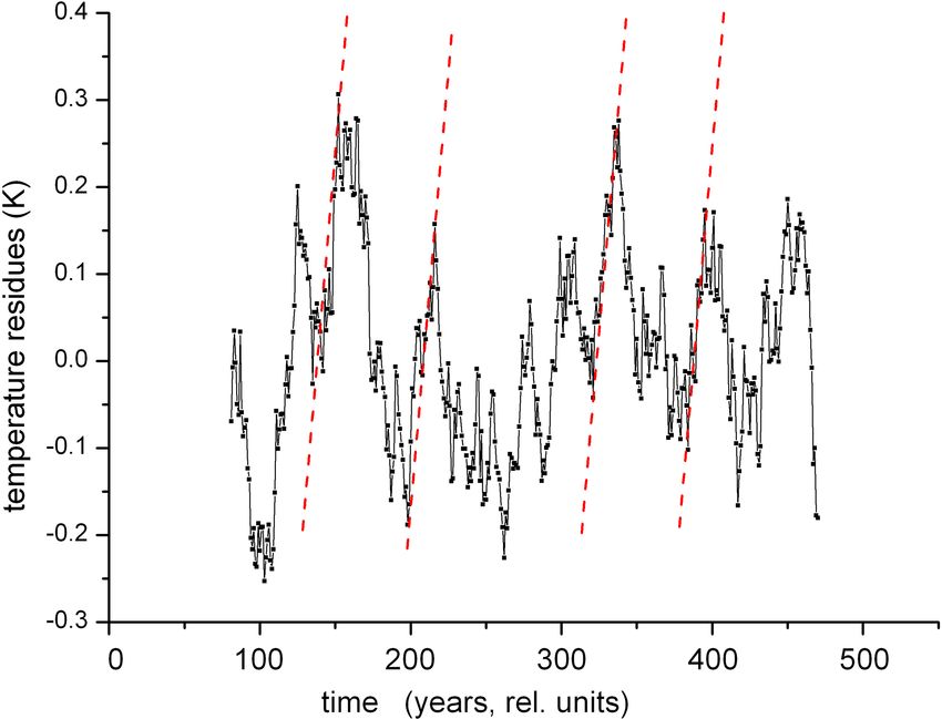
D. Offermann et al.: Very long period oscillations in the atmosphere (0–110 km) – Part 2                                         3269

Table 1. Oscillation periods and their standard deviations at 50◦ N,   harmonic analysis and yields estimated values for amplitudes
7◦ E vs. 50◦ S, 7◦ E (HAMMONIA model). Bold font indicates             and phases of the oscillation at these altitudes. Details are
agreement of periods within combined standard deviations.              given by Offermann et al. (2021). The statistical significance
                                                                       of the period values presented in this paper has been analysed
         Period   SD     Period     SD    Difference   Combined        in the preceding paper of Offermann et al. (2021, Sect. 3.2).
           (yr)            (yr)           of periods     SD
         50◦ N            50◦ S
    1     5.34 ± 0.1       5.61 ± 0.15        −0.27       0.25         2.1   Periods
    2     6.56 0.24
    3     7.76 0.29        7.42    0.28        0.34       0.57         The above-mentioned nine periods found by Offermann et
    4     9.21 0.53        9.24    0.45       −0.03       0.98         al. (2021) are repeated in Table 1 together with their stan-
    5     10.8 0.34        10.7    0.18         0.1       0.52         dard deviations (SD). At 50◦ S, our analysis obtains seven
    6     13.4 0.68        13.2    0.86         0.2       1.54
                                                                       oscillations that are also shown in Table 1. They all find a
    7     17.3 1.05        16.5     1.3         0.8       2.35
    8     22.8 1.27           –       –                                correspondence in the northern values. A close agreement is
    9     28.5 1.63        30.3     4.6        −1.8       6.23         found that is well within the combined standard deviations in
                                                                       all but one case and is even within a single standard devia-
                                                                       tion in most cases. These cases are indicated in bold font in
the behaviour of the cold-point tropopause is discussed. Sec-          Table 1.
tion 5 summarizes the results.                                            Table 1 holds a twofold surprise: first, it is interesting to
                                                                       see that long-period oscillations exist in the Southern Hemi-
                                                                       sphere and also in the Northern Hemisphere. Second, it is
2       HAMMONIA model (Hamburg Model of the Neutral                   surprising that the values of the periods are so nearly the
        and Ionized Atmosphere)                                        same. We would not expect this if the surface–atmosphere
                                                                       interaction did play a significant role. This is apparently not
The HAMMONIA model (Schmidt et al., 2006) is based
                                                                       the case. Our data rather appear to hint at a global-oscillation
on the ECHAM5 general-circulation model (Roeckner et
                                                                       mode that shows up in several periods.
al., 2006) and extends vertically to 110 km. The simulation
analysed here was run at a spectral resolution of T31 with
119 vertical layers. A 34-year run of the model (38 123)               2.2   Amplitudes
has been analysed here for long-period oscillations at Wup-
pertal (50◦ N, 7◦ E). Model details and harmonic-oscillation           The vertical amplitude profile in Fig. 1 shows a pronounced
analysis have been described in Offermann et al. (2021).               structure. This offers a valuable tool for our north–south
Model boundaries with respect to the sun, ocean, and green-            comparison. Offermann et al. (2021) showed that vertical
house gases were held constant. Nine long-period oscilla-              amplitude profiles of the different oscillation periods were
tions with periods between 5 and 28 years have been de-                surprisingly similar at the northern location. Their maxima
tected (see Table 1). They were discussed in terms of self-            occurred at about the same altitudes and so did the minima.
excited (internal) atmospheric oscillations. Doubts concern-           (See the accumulated amplitudes in Fig. 11 of that paper.)
ing the self-excitation remained, however, because a possible          As a consequence, the temperature standard deviations can
land surface–atmosphere interaction could not be excluded.             be used as proxies for the accumulated amplitudes. This is
We therefore perform a corresponding analysis here for a               done for the location at 50◦ N, 7◦ E in Fig. 2 (black squares).
conjugate geographic point at 50◦ S, 7◦ E. This location is            For the southern location at 50◦ S, 7◦ E, we do the same for
about 15◦ S of the southernmost tip of South Africa in the             a comparison to the north (Fig. 2, red dots).
middle of the ocean. Hence, the surface–atmosphere interac-               In the paper of Offermann et al. (2021), it was shown that
tion should be quite different here from that in the middle of         the occurrence of the long-period oscillations was clearly de-
Europe. In case such an interaction plays a role, we hope to           pendent on the direction of the zonal wind: strong oscillation
see this by comparing various atmospheric parameters. The              activity was not observed for easterly (westward) winds. In
analysis procedures in the north and the south are exactly the         the middle atmosphere, the zonal wind during solstices is op-
same.                                                                  posite in the Northern and the Southern Hemisphere. Hence,
   Following Fig. 1, we study periods and amplitudes of the            comparison of annual mean amplitudes at 50◦ N and 50◦ S
long-period oscillations. The figure shows that there are al-          could be misleading. Here, we therefore compare data of
titude ranges where a period could not be detected. This is            the same season: January at 50◦ N to July at 50◦ S (Fig. 2;
attributed to the fact that the oscillation was not excited here       zonal wind is eastward) and July at 50◦ N to January at 50◦ S
or that it was too strongly damped to be detected (see Offer-          (Fig. 3; zonal wind is westward).
mann et al., 2021). At these altitudes, the mean period value             As expected, a comparison of the two pictures shows a
of the other altitudes is used as a proxy (dashed vertical red         large difference in the profiles between summer and winter
line, 17.3 ± 0.79 yr in Fig. 1). The proxy is entered into the         at a given latitude because of the opposite wind directions.

https://doi.org/10.5194/acp-23-3267-2023                                               Atmos. Chem. Phys., 23, 3267–3278, 2023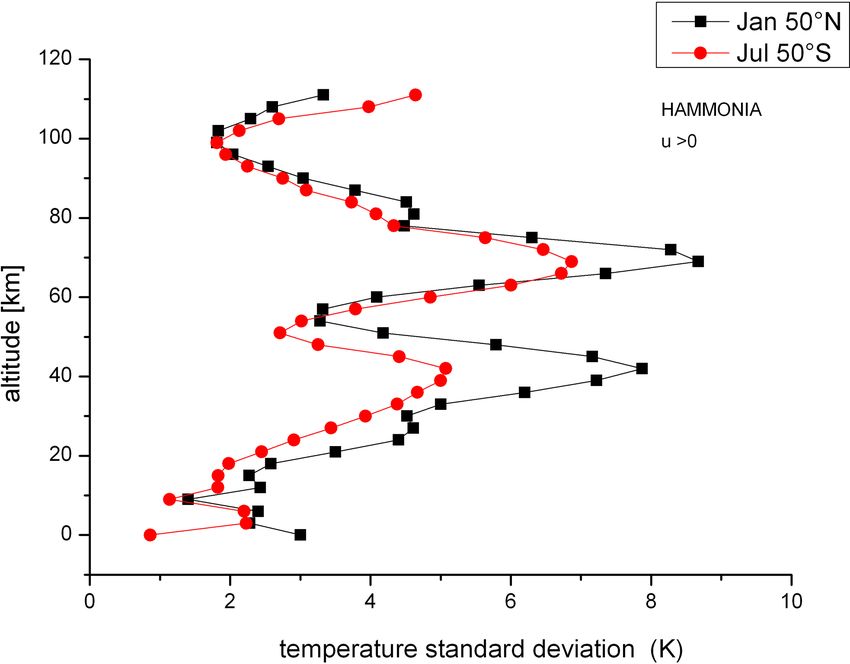
3270                                  D. Offermann et al.: Very long period oscillations in the atmosphere (0–110 km) – Part 2

                                                                       Table 2. Oscillation periods and their standard deviations at 50◦ N,
                                                                       7◦ E vs. 50◦ S, 7◦ E (ECHAM6 model). Bold font indicates agree-
                                                                       ment of periods within combined standard deviations.

                                                                                 Period    SD    Period    SD     Difference   Combined
                                                                                   (yr)            (yr)           of periods        SD
                                                                                 50◦ N            51◦ S
                                                                           1       20 ± 0.35       20.1 ± 0.4         −0.1          0.75
                                                                           2       20.9 0.15       21.8 0.37          −0.9          0.52
                                                                           3       22.1 0.23       23.2 0.33          −1.1          0.56
                                                                           4       23.8 0.42       24.3 0.41          −0.5          0.83
                                                                           5       25.3 0.46       26.1 0.44          −0.8           0.9
                                                                           6       27.3 0.41       28.6 0.44          −1.3          0.85
                                                                           7       30.2 0.49       31.8 0.58          −1.6          1.07
                                                                           8       33.3 0.84       34.5 0.58          −1.2          1.42
                                                                           9       36.9 1.17       38.3 1.05          −1.4          2.22
                                                                           10      41.4 0.97         43 1.52          −1.6          2.49
                                                                           11      48.4 1.73       49.7 1.78          −1.3          3.51
Figure 2. Temperature standard deviations as proxies for oscillation       12      58.3 1.77       60.3 2.33           −2            4.1
                                                                           13      64.9 2.98       66.5     2.5       −1.6          5.48
amplitudes in winter. Data for January at 50◦ N (black squares) are
                                                                           14      77.5 3.94       84.8 4.74          −7.3          8.68
compared to July at 50◦ S (red dots).
                                                                           15      95.5 5.86      110.9 10.9         −15.4         16.76
                                                                           16     129.4 14.5      160.2 8.88         −30.8         23.38
                                                                           17     206.7 16.3

                                                                       3        ECHAM6 model (ECMWF Hamburg)

                                                                       Much longer periods than those in HAMMONIA were found
                                                                       in the ECHAM6 model (Offermann et al., 2021). ECHAM6
                                                                       is the successor of ECHAM5 (Stevens et al., 2013). As the
                                                                       atmospheric component of the Max Planck Institute Earth
                                                                       system model (MPI-ESM; Giorgetta et al., 2013), it has
                                                                       been used in a large number of model intercomparison stud-
                                                                       ies related to the Coupled Model Intercomparison Project
                                                                       phase 5 (CMIP5). The ECHAM6 simulation analysed here
                                                                       was run at T63 spectral resolution with 47 vertical layers.
                                                                       For more details, see Offermann et al. (2021).
                                                                          Our analyses were based on a 400-year run of the
Figure 3. Temperature standard deviations as proxies for oscillation   ECHAM6 model. In the long-period range, 17 oscillations
amplitudes in summer. Data are for July at 50◦ N (black squares)       were observed between 20 and 206 years (Table 2). They
and for January at 50◦ S (red dots).                                   offer further north–south comparisons in the multi-decadal
                                                                       range and beyond.

The profiles in the same season, however, are surprisingly
similar at 50◦ N and 50◦ S.                                            3.1       Periods
   Taking together the results of periods and amplitudes, it
appears that we see essentially the same atmospheric be-               A harmonic analysis of the 400-year run at 50◦ S, 7◦ E is
haviour at 50◦ N and 50◦ S. We see no evidence of a possible           performed in the same way as described in Offermann et
interaction between the land surface and the atmosphere in             al. (2021) for the north. Sixteen periods can be identified
the excitation of the oscillations, as the corresponding pro-          here, with periods between 20 and 160 years. These are com-
files are so similar. We therefore tend to believe that these          pared to the northern values in Table 2. (In some places of
oscillations are self-excited (internal). A deviation from this        Tables 1–4, periods (counterparts) are missing. It is believed
similarity occurs, however, at the lowest altitude in Figs. 2          that, in these cases, the amplitudes were too small to be de-
and 3. This will be discussed in Sect. 4 below.                        tected, as mentioned.)
                                                                          We find corresponding oscillation values (“north–south
                                                                       pairs”) in all cases except one (206.7 year in the north). The
                                                                       second last column of Table 2 shows the pair differences, and

Atmos. Chem. Phys., 23, 3267–3278, 2023                                                    https://doi.org/10.5194/acp-23-3267-2023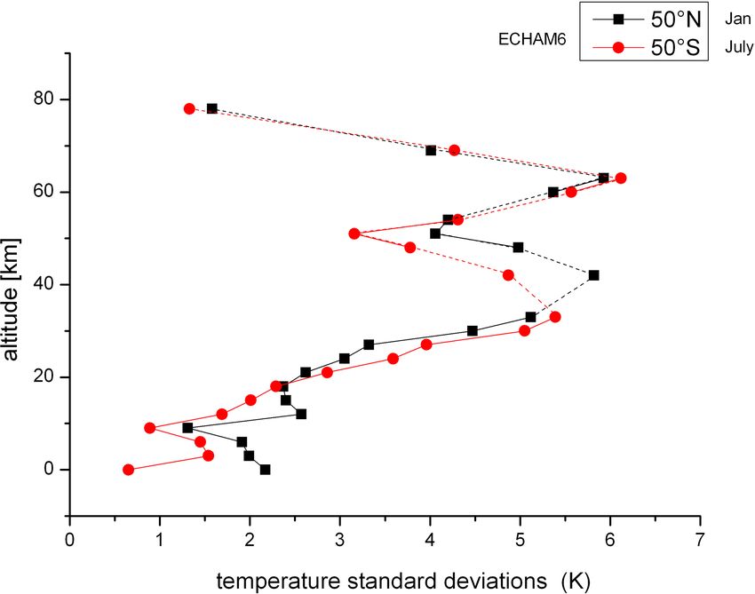
D. Offermann et al.: Very long period oscillations in the atmosphere (0–110 km) – Part 2                                              3271

Table 3. Temperature oscillation periods (year) at 50◦ N, 7◦ E; standard deviations (SD); and column differences. Bold font indicates agree-
ment of periods within combined standard deviations.

                                 Period     SD     Period       SD    Period       SD    Difference     SD sum
                                 annual           January               July                Jan–Jul    Jan + Jul
                           1        20     0.35      19.6     0.33      19.8     0.52          −0.2         0.85
                           2       20.9    0.15      20.8     0.32        21     0.18          −0.2          0.5
                           3       22.1    0.23      22.4     0.33      22.2     0.38           0.2         0.71
                           4       23.8    0.42      24.1     0.19      24.1     0.31             0          0.5
                           5       25.3    0.46      25.3     0.49      26.1     0.21          −0.8          0.7
                           6       27.3    0.41      27.8     0.76      27.7     0.17           0.1         0.93
                           7       30.2    0.49      30.3     0.62      30.2     0.76           0.1         1.38
                           8       33.3    0.84      33.1     1.03      33.7     0.55          −0.6         1.58
                           9       36.9    1.17      37.5     1.05      38.1      1.3          −0.6         2.35
                           10      41.4    0.97      41.5     1.49      44.3     1.23          −2.8         2.72
                           11      48.4    1.73      48.3     1.69         –        –             –            –
                           12      58.3    1.77      57.9     0.53      53.3     1.77           4.6          2.3
                           13      64.9    2.98      63.5      2.7      66.2     1.92          −2.7         4.62
                           14      77.5    3.94      77.1      2.5      79.1     5.11           −2          7.61
                           15      95.5    5.86      97.6     7.81     103.8      5.4          −6.2        13.21
                           16     129.4    14.5     130.1     9.03     121.1     9.32             9        18.35
                           17                       169.3    10.55     183.4     7.51         −14.1        18.06
                           18     206.7    16.3      239      15.3     216.2    14.67          22.8        29.97

the last column shows the combined standard deviations. An              3.2    Amplitudes
agreement of periods within the combined standard devia-
tions is found in 11 cases (in bold font). In the remaining five        Amplitudes of the long-period oscillations found in
cases, the periods agree within twice the standard deviations.          ECHAM6 are analysed in terms of temperature standard de-
This close agreement of the N–S pairs is similar to that given          viations, as has been done for the shorter periods of the
in Table 1. It is very remarkable that this close correspon-            HAMMONIA model. Also here, large seasonal differences
dence exists at these much longer periods, too. Together with           are expected. Therefore, a north–south comparison is per-
the HAMMONIA results, this again suggests some kind of a                formed for corresponding seasons, i.e. January north is com-
three-dimensional global-oscillation mode.                              pared to July south as an example for winter. July north and
   The HAMMONIA data show substantial differences in                    January south are compared correspondingly for summer.
terms of oscillation amplitudes between summer and win-                 This is shown in Figs. 4 and 5, respectively.
ter. The oscillation periods of HAMMONIA and ECHAM6                        Large seasonal differences are seen, indeed, and are simi-
in Tables 1 and 2, respectively, are annual values. As north            lar to those in the shorter periods in Figs. 2 and 3. North and
and south are opposite in season, the good agreement of the             south profiles are, however, very similar if the same seasons
corresponding period pairs suggests that seasonal differences           are considered, as is observed for the shorter periods. Again,
of the periods should not be large. We verify this using the            similarity is clearly lost at the lowest altitude.
larger set of ECHAM6 data. We compare annual mean oscil-                   It is also remarkable that the maxima near 40 and 70 km
lation periods to January and July (mean) values, respectively          agree so well in Figs. 2 and 4.
(Table 3).
   The comparison of the results at 50◦ N between annual                3.3    Seasonal differences
periods and corresponding periods in the January data at
50◦ N yields 16 coincidences which agree within the com-                If there were an appreciable influence of land surface and
bined standard deviations. The corresponding analysis of the            vegetation on the excitation of the long-period temperature
annual 50◦ S data (Table 2) and the July data at 50◦ S gives            oscillations in the atmosphere, one would expect a differ-
13 coincidences, 12 of which agreed within the combined                 ence of the oscillations in relation to season at a given lo-
standard deviations. (One agrees within the double standard             cation. Such an analysis is in part implicitly contained in the
deviations.) Hence, there is no essential difference between            north–south comparisons given above. We repeat it here in
the annual and the summer and/or winter oscillation periods.            more detail. Oscillation periods in January (northern hemi-
                                                                        spheric winter) and July (northern hemispheric summer) are
                                                                        analysed in the ECHAM6 model at 50◦ N, 7◦ E. Seventeen
                                                                        pairs of oscillation periods can be identified at values similar

https://doi.org/10.5194/acp-23-3267-2023                                                 Atmos. Chem. Phys., 23, 3267–3278, 2023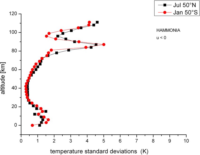
3272                                 D. Offermann et al.: Very long period oscillations in the atmosphere (0–110 km) – Part 2

                                                                     Figure 6. Long-period temperature oscillations in the ECHAM6
Figure 4. Comparison of ECHAM6 temperature standard devia-
tions in winter. January 50◦ N (black squares) and July 50◦ S (red   model at 50◦ N, 7◦ E. Accumulated amplitudes are shown vs. al-
dots) are given as examples.                                         titude for the periods given in Table 3. Black squares are from
                                                                     monthly mean January data. Red bullets are from July.

                                                                     tions. The agreement of the monthly periods with the annual
                                                                     ones (first column in Table 3) is similarly close.
                                                                        Given the close agreement of the monthly periods, it is
                                                                     interesting to compare their amplitudes.
                                                                        These are shown in Fig. 6. Accumulated amplitudes are
                                                                     shown, i.e. the sum of all oscillation amplitudes obtained at a
                                                                     given altitude. The amplitudes could not be derived for each
                                                                     altitude. Hence, the curves shown in Fig. 6 are approximate.
                                                                     The two curves are quite different. The January curve has
                                                                     high values, is highly structured, and closely resembles in
                                                                     shape the winter temperature standard deviation profiles in
                                                                     Fig. 4. The values of the July curve are much smaller and
                                                                     resemble in shape the summer curves of the standard devia-
                                                                     tions given in Fig. 5. These agreements again justify the use
                                                                     of temperature standard deviations as proxies of the oscilla-
                                                                     tion amplitudes.
Figure 5. Comparison of ECHAM6 temperature standard devia-
                                                                        The large difference in amplitudes in summer and winter
tions in summer. July 50◦ N (black squares) and January 50◦ S (red
circles) are given as examples.                                      in the stratosphere and mesosphere may be attributed to the
                                                                     opposite direction of zonal winds in the middle atmosphere
                                                                     in these seasons. It is surprising that, in spite of these large
                                                                     differences, the periods of the oscillations are so nearly the
to those of the annual analysis shown in the first column of         same. This demonstrates that the oscillation period is a robust
Table 2. This is shown in Table 3. Standard deviations (SD)          parameter, as has been discussed by Offermann et al. (2021).
of the periods are also given. A period near 48 years could
not be found in July. These results are compared to the an-
nual values of Table 2. The second-to-last column in Table 3         3.4   High latitudes
shows the differences of the periods in January and July. The
last column shows the sum of their standard deviations. A            Considerable land surface and vegetation differences might
close agreement of the January and July periods is found:            also be expected at polar latitudes. We have therefore
in 14 cases, the periods agree within the combined stan-             analysed ECHAM6 temperatures at 75◦ N, 70◦ E (northern
dard deviations, which is indicated by bold font in Table 3          Siberia) and 75◦ N, 280◦ E (northernmost Canada). Winter
(12 cases agree even within single standard deviations). In          temperatures (January) have been searched for long-period
three cases, the periods agree within double standard devia-         oscillations in the same way as described above. The results

Atmos. Chem. Phys., 23, 3267–3278, 2023                                               https://doi.org/10.5194/acp-23-3267-2023
D. Offermann et al.: Very long period oscillations in the atmosphere (0–110 km) – Part 2                                          3273

Table 4. Temperature oscillation periods (year) and their standard
deviations (SD) at 50◦ N, 7◦ E; 75◦ N, 70◦ E; and 75◦ N, 280◦ E in
January.

          50◦ N,      SD    75◦ N,     SD    75◦ N,       SD
            7◦ E             70◦ E           280◦ E
    1       19.6     0.33     19.6    0.44      19.2     0.26
    2       20.8     0.32       21    0.19      20.7     0.32
    3       22.4     0.33     22.8     0.4      22.6     0.32
    4       24.1     0.19     24.4     0.2      24.4      0.3
    5       25.3     0.49     25.8    0.55      25.3     0.27
    6       27.8     0.76     28.9    0.34      26.7     0.29
    7       30.3     0.62     30.9    0.66      29.9      0.7
    8       33.1     1.03     33.1    0.51      32.6     0.69
    9       37.5     1.05     35.8    0.93        37      0.6
    10      41.5     1.49     40.5     0.9      39.7      0.8
    11                        44.7    1.25      43.9     1.29
    12      48.3    1.69      51.1    2.22      50.9     2.49        Figure 7. Temperature standard deviations at polar latitudes –
    13      57.9    0.53                                             75◦ N, 280◦ E (black squares) and 75◦ N, 70◦ E (red dots) – in Jan-
    14      63.5     2.7      61.4    1.75      64.4     2.73        uary.
    15      77.1     2.5      76.7    4.04      82.2     2.16
    16      97.6    7.81      95.8    5.97      91.2     5.91
    17     130.1    9.03     149.4    9.95     139.4    10.99        4     Discussion
    18     169.3   10.55
    19       239    15.3     232.5    13.1     244.5     22.8        4.1    Internal oscillations
                                                                     The boundary conditions of the computer model runs used by
                                                                     Offermann et al. (2021) and in the present analysis were kept
are shown in Table 4. For comparison, January data at 50◦ N          constant. This concerned solar irradiation, the ocean, and
from Table 3 are also given.                                         greenhouse gases. Nevertheless, the atmospheres in the mod-
   The results are quite interesting. The periods found at the       els showed pronounced and consistent oscillations. It was
two polar locations are very similar. Seventeen periods have         therefore suggested that these oscillations were self-excited
been found at either station, and 16 of these agree within the       or internal in the atmosphere. Land surface and vegetation
combined standard deviations (12 agree even within single            changes as external influences, however, were not completely
standard deviations). The periods at high latitudes are quite        excluded in the earlier paper. To check such possible influ-
similar to those at middle latitudes (50◦ N, 7◦ E). The 18 peri-     ences, the models are analysed here at times and locations
ods seen at 50◦ N find 16 counterparts in either high-latitude       that have different land surface and vegetation conditions.
station. Of these 15, 14 agree within the combined standard          These are, on the one hand, two corresponding locations
deviations for the 70◦ E (280◦ E) station. Eleven periods even       in the Northern and Southern Hemispheres (50◦ N and S at
agree within single standard deviations in either case. Hence,       7◦ E). On the other, hand two different seasons are compared
the comparison of middle to high latitudes does not show an          at the same location (50◦ N, 7◦ E). Finally, two polar loca-
influence on periods, either.                                        tions (75◦ N at 70 and 280◦ E, respectively) are compared to
   Deser et al. (2012) showed in their analysis that the vari-       the middle latitudes.
ability of surface temperatures at high (northern) latitudes            The results for all northern and southern locations and
was considerably larger than that at middle and low latitudes.       occasions are very similar as concerns the oscillation peri-
A similar result is obtained in the present data set for the up-     ods. Pairs of oscillations at two different locations are com-
per atmosphere. We have calculated the temperature standard          pared and show nearly the same values in many cases. Also,
deviations at the two polar locations (75◦ N) and show them          the amplitudes are found to be similar when comparing the
in Fig. 7. The results at the 70 and 280◦ E longitudes are           corresponding seasons. However, amplitudes during differ-
fairly similar. However, as suspected, they are significantly        ent seasons (summer and winter) at the same location are
larger than the mid-latitude values shown in Fig. 4.                 quite different. Despite this discrepancy, their periods are
   The profile forms shown in Fig. 7 are fairly different from       very similar. We conclude from these various similarities that
those in Fig. 4. They are smeared, and the extrema occur at          the long-period oscillation are not likely to originate from
different altitudes. It appears that the profiles for different      land surface and vegetation processes in most parts of our
oscillation periods can be different for different latitudes, as     high vertical profiles. However, the similarity is lost at the
well as for different longitudes. A detailed analysis is, how-       lowest altitude, as mentioned above.
ever, beyond the scope of this paper.

https://doi.org/10.5194/acp-23-3267-2023                                             Atmos. Chem. Phys., 23, 3267–3278, 2023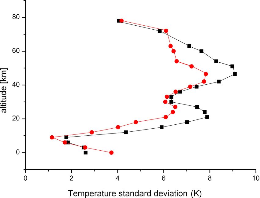
3274                                D. Offermann et al.: Very long period oscillations in the atmosphere (0–110 km) – Part 2

    The large summer–winter difference in amplitudes (stan-
dard deviations) is shown here for one pair of north–south
locations (50◦ N and S, 7◦ E) only. Deser et al. (2012) have
shown global surface analyses which indicate, however, that
this may be a global phenomenon (their Fig. 16). This is seen
if their December–January data are compared to our January
data: northern values are much larger than southern values.
It thus appears that our north–south difference is part of an
extended (global) structure.
    However, there is a seeming disagreement between our
data and those of Deser et al. (2012) in July: theses authors do
not see much difference between 50◦ N and 50◦ S, whereas
here in Figs. 2–5 the northern values are much smaller than
those in the south if the entire profiles are considered.
    The discrepancy disappears if only the lowest altitudes in
our data are considered. Our north and south profiles are
fairly similar at all altitudes, except in the case of the bot-     Figure 8. ECHAM6 annual temperature residues at 50◦ N, 7◦ E and
tom values: at the lowest altitude, all of our southern ampli-      18 km altitude. Data have been smoothed by a 16-point running
tudes (given as standard deviations) are much smaller than          mean. Time is in relative units. Inclined dashed (red) lines have a
their northern counterparts (Figs. 2–5). It needs to be em-         gradient of 0.2 K per decade.
phasized that this difference is limited to the lowermost al-
titude and disappears at about the next higher level (3 km).
This applies to the two different models HAMMONIA and               4.2     Implications of internal oscillations
ECHAM6. The difference of the two lowermost levels is sur-
prising. It is, however, significant, as the statistical error of   4.2.1     Temperature trends
the standard deviations is 12 % for HAMMONIA and 3.5 %
for ECHAM6. In numbers, Figs. 2–5 yield the following re-           Long-term temperature changes are part of the ongoing cli-
sults. The January values are high in the north (2.2–3.0 K)         mate change in the troposphere and in the upper atmosphere
and small in the south (0.39–0.68 K). Contrary to this, the         (Eyring et al., 2021). It is important to know whether there
July values are comparatively low in the north (1.04–1.12 K)        is a relationship between these trends and the internal (non-
and in the south (0.65–0.86 K). This is qualitatively similar       anthropogenic) atmospheric variability. We study this ques-
to the results of Deser et al. (2012).                              tion by means of ECHAM6 data in the lower stratosphere,
    Desai et al. (2022) mention that land–atmosphere inter-         as the boundary values of the model runs were kept constant,
actions should occur essentially in the lowest 1–2 km of            and therefore the model variability is believed to be internal.
the atmosphere (boundary layer). It thus appears interest-             New long-term temperature trends in the troposphere
ing to interpret the large deviations from profile similarity at    and stratosphere have recently been presented by Steiner
the lowermost levels of Figs. 2–5 as an indication of land–         et al. (2020). Data cover about four decades (1980–2020).
atmosphere interaction at these levels. The deviations are          These authors find trends on the order of −0.2 K per decade
large and significant. They quickly disappear at the higher         in the lower stratosphere (near-global averages; their Fig. 8).
levels. This suggests that excitation of long-period oscilla-       For comparison, we show ECHAM6 data for 50◦ N, 7◦ E at
tions by land surface–atmosphere interactions would be lim-         18 km altitude in our Fig. 8. These data are annual mean
ited to the lowermost atmosphere.                                   residues; i.e. the mean value has been subtracted from the
    Internal variability in the atmosphere has been discussed       annual data set. The series has been smoothed by a 16-point
several times in the literature (see Deser, 2020, and refer-        running mean. The figure shows trend-like increases or de-
ences therein). This is thought to be caused by the chaotic         creases of 0.2 K per decade or even steeper over 4-decade
dynamics of the atmosphere and oceans and to be generally           intervals. This is indicated by the slanted red lines that give
unpredictable more than a few years ahead of time. It remains       an increase of 0.2 K per decade.
to be determined how this is related to our internal oscilla-          The comparison with Steiner et al. (2020) is approx-
tions.                                                              imate because our data are local (50◦ N, 7◦ E), whereas
                                                                    Steiner et al. (2020) give global means. Such means tend
                                                                    to smooth all variability to some extent. Nevertheless, the
                                                                    results suggest that the long-term trends derived by Steiner
                                                                    et al. (2020) may contain some contribution of internal
                                                                    (i.e. non-anthropogenic) variability. This confirms a corre-
                                                                    sponding result of these authors saying that “. . . there may be

Atmos. Chem. Phys., 23, 3267–3278, 2023                                                https://doi.org/10.5194/acp-23-3267-2023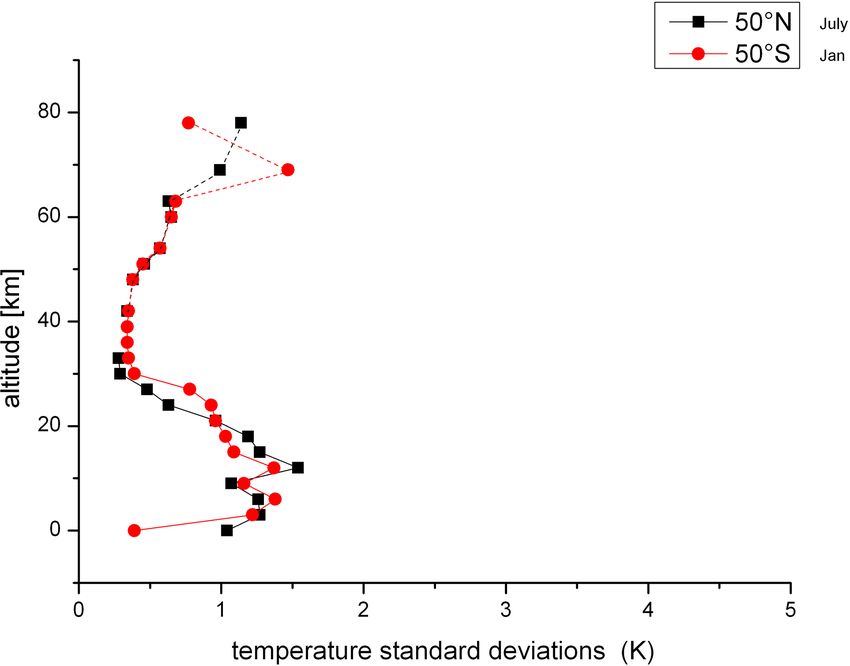
D. Offermann et al.: Very long period oscillations in the atmosphere (0–110 km) – Part 2                                           3275

a non-negligible internally generated component to the larger
stratospheric trends . . . ” (see their Sect. 5).
   Care must therefore be taken if deriving climate trends
from data sets of limited length (4 decades).
   A similar caveat applies if internal oscillations with peri-
ods on this order are excited in the atmosphere.

4.2.2   Cold-point tropopause

The cold-point tropopause (CPT) is frequently discussed as a
climate indicator (see e.g. Hu and Vallis, 2019; Gettelman et
al., 2009; Han et al., 2017). A similar parameter is the lapse
rate tropopause (LRT), which we do not discuss here, as it is
generally close to and behaves similarly to the CPT (Pan et
al., 2018; RavindraBabu et al., 2020).
   We analyse long-term changes of the cold-point
tropopause (CPT) in the ECHAM6 model with fixed                     Figure 9. Cold-point tropopause temperatures in ECHAM6. Win-
boundaries at 50◦ N, 7◦ E and the corresponding Southern            ter data are shown for 50◦ N, January (black) and 50◦ S, July (red).
Hemisphere location (50◦ S, 7◦ E) as part of our north–south        Dotted vertical lines (black) indicate a 60-year periodicity. Inclined
comparison. The lowest temperatures are found in this model         dashed lines (blue) show a trend of 1 K per decade. Time is in rela-
at 11.5 km (208.67 hPa) and 12.4 km (181.16 hPa; this is the        tive units.
altitude resolution of the data). We have selected the lowest
temperature at these two altitudes and thus formed a data           Table 5. Cold-point tropopause oscillations in winter at 50◦ N and
set that approximates the cold-point tropopause, considering        51◦ S, standard deviations, and column differences. Bold font indi-
our limited altitude resolution.                                    cates agreement of periods within combined standard deviations.
   The results are shown in Fig. 9. The figure compares our
CPT data at the two locations. To study data that correspond,               CPT       SD       CPT      SD    Difference     Combined
winter values are shown, i.e. January data in the Northern                 period            period           of periods          SD
                                                                             (yr)               (yr)
Hemisphere and July data in the Southern Hemisphere. The
                                                                              Jan                Jul
data have been smoothed by a 16-point running mean to                      50◦ N              51◦ S
suppress the short-term variability that is large (5 K peak to
peak). The picture shows that the southern CPT are some-             1       19.8    0.27      20.2    0.56         −0.4          0.83
                                                                     2       21.1    0.44      22.2    0.38         −1.1          0.82
what lower than the northern ones. Most interesting is the
                                                                     3       24.9    0.32      24.1    0.38          0.8           0.7
strong variability in either data set, including some apparent       4       28.8    1.26      26.2    0.32          2.6          1.58
periodicity. The latter is indicated by the vertical dashed lines    5       31.3    1.84      32.8     0.6         −1.5          2.44
at 60-year intervals.                                                6       42.3    1.64      39.8    1.33          2.5          2.97
   On timescales of decades, positive and negative trends are        7       48.3    3.22      47.1    3.22          1.2          6.44
seen. The positive trends are comparable to the dashed (blue)        8         58    2.22      65.5    2.14         −7.5          4.36
straight lines that have a gradient of 1 K per decade. The pic-      9       75.1    4.45      81.8     5.6         −6.7         10.05
ture shows that such gradients or even steeper ones are not          10     107.7    6.64      96.4     8.7         11.3         15.34
                                                                     11     179.3    13.3     171.5    21.7          7.8            35
uncommon in the data. The decreasing branches show simi-
lar (negative) gradients.
   Gradients on this order of magnitude are reported in
the literature. Amazingly, both positive and negative val-          respectively. It was shown above that there is little difference
ues are found, as mentioned in Sect. 1. Recently, negative          between annual and monthly oscillation periods, and it was
and positive trends in two subsequent 20-year time intervals        checked that this applies here, too.
(1980–2000; 2001–2020) have been discussed by Konopka                  Indeed, the harmonic analyses of the data yield a number
et al. (2022). Figure 9 shows that this may not be surprising       of internal oscillation periods in the period range of Table 2.
but may occur quite naturally depending on the time interval        The results at the northern and southern locations are com-
chosen for the trend determination. The quasi-periodic be-          pared in Table 5. The table shows that the periods in the north
haviour of the CPT plays a role here and suggests a possible        and south form pairs similarly to those in Tables 1 and 2. A
connection to the internal oscillations of the atmosphere.          total of 11 coincidences are obtained. Seven of these agree
   We therefore perform harmonic analyses of the CPT data           within the combined standard deviations (bold font in the
similarly as those described above for annual temperatures in       last two columns of Table 5). Four agree within the double
Table 2. The CPT data are monthly data of January and July,         standard deviations. All periods listed in Table 5 also find a

https://doi.org/10.5194/acp-23-3267-2023                                             Atmos. Chem. Phys., 23, 3267–3278, 2023
3276 D. Offermann et al.: Very long period oscillations in the atmosphere (0–110 km) – Part 2
counterpart in the corresponding (north or south) columns It is therefore concluded that the oscillations most likely are
of Table 2. Also, these pairs agree within combined stan- internally excited in the atmosphere.
dard deviations (except one). It thus appears that the cold- There is, however, one exemption. Land–atmosphere in-
point tropopause is at least partly controlled by the internal teractions should mainly occur in the lowermost atmosphere
atmospheric oscillations. This applies to the north and also to (boundary layer). We therefore considered especially the
the south; i.e. the north–south symmetry shown above is also lowest atmospheric levels. Here, indeed, the vertical ampli-
found in this parameter. tude profiles showed peculiar structures that we tentatively
The amplitudes of the CPT oscillations are found to be attribute to land–atmosphere interactions. The peculiarities
quite variable with the period (not shown here). The northern quickly disappear at higher altitudes. Hence, we obtain the
and the southern data both show strong amplitude peaks near preliminary picture of self-excited oscillations in the upper
60 years. This fits with the data shown in Fig. 9. atmosphere and possible land surface excitation at the lowest
Low-frequency oscillations (LFO) in the multi-decadal levels.
range (50–80 years) have frequently been discussed for
surface temperatures. They have, for instance, been inter- 5.2 Trends and long periods
preted as internal Atlantic multidecadal variability or Pa-
cific decadal oscillations and interdecadal Pacific oscillations Long-term trends in atmospheric parameters are frequently
(e.g. Meehl et al., 2013, 2016; Lu et al., 2014; Deser et al., analysed in the context of the ongoing climate change. Trend
2014; Dai et al., 2015). It appears that internal oscillations values are mostly small, and it is sometimes difficult to de-
also play a role here as contributors to the CPT variations in termine whether or to what extent they are anthropogenic in
either hemisphere. Great caution is therefore advised when nature. In this context, internal oscillations can play a role,
interpreting tropopause changes in the context of the anthro- even if their amplitudes are small. If the oscillation period
pogenic long-term climate changes (e.g. Pisoft et al., 2021). is on the order of the interval used for the trend analysis, it
may become difficult to disentangle trend and oscillation. It
is unimportant here whether the oscillations are self-excited
5 Summary and conclusions or not.
As an example, the cold-point tropopause (CPT) in the
5.1 Self-excitation of oscillations 400-year run of the ECHAM6 model with fixed boundaries
is analysed at two north–south locations. Strong trend-like
Present-day sophisticated atmospheric computer models ex- increases or decreases of CPT values are seen on decadal
hibit long-period temperature oscillations in the multi- timescales (order of 30 years). They are on the order of the
annual, decadal, and even centennial year range. Such os- trend values discussed in the literature. They are, however,
cillations may be found even if the model boundaries are not of anthropogenic origin, as is frequently assumed in the
kept constant concerning the influences of solar radiation, the literature. Harmonic analysis of the CPT values yields oscil-
ocean, and the variations of greenhouse gases (Offermann lation periods that are very similar for the north and south
et al., 2021). A possible influence of land surface and veg- locations and are similar to the values otherwise given in this
etation changes, however, was yet undecided. Therefore, in analysis. Apparently, these internal oscillations are important
the present analysis, oscillation periods are compared at lo- contributors to the CPT variations observed.
cations and occasions with different land surface and vege-
tation behaviour with the hope of seeing possible differences
in oscillation periods. Three cases are studied: first, a loca- Data availability. The HAMMONIA and ECHAM6 data are
tion in the Northern Hemisphere (50◦ N, 7◦ E) and its coun- available from Hauke Schmidt, MPI Meteorology, Hamburg.
terpart in the Southern Hemisphere (50◦ S, 7◦ E) are con-
sidered. The northern location is in the middle of Europe,
whereas the southern location is 15◦ S of the tip of South Author contributions. DO performed the data analysis and pre-
pared the paper with the help of all co-authors. JW managed the
Africa in the middle of the Southern Ocean. Second, two dif-
data collection and preparation. CK helped with the geographical
ferent seasons are compared in the northern location (January analysis. RK provided interpretation and editing of the paper.
and July). Third, two polar latitude locations are studied at
75◦ N, 280◦ E and 75◦ N, 70◦ E. The land surface and vege-
tation conditions are quite different in all of these cases. Competing interests. The contact author has declared that none
Two models are studied (HAMMONIA, ECHAM6) for of the authors has any competing interests.
medium and long oscillation periods (5 to beyond 200 years).
The periods obtained for the contrasting cases are all found
to be very similar. Disclaimer. Publisher’s note: Copernicus Publications remains
The same holds for the vertical profiles (up to the neutral with regard to jurisdictional claims in published maps and
mesopause) of the oscillation amplitudes at most altitudes. institutional affiliations.
Atmos. Chem. Phys., 23, 3267–3278, 2023 https://doi.org/10.5194/acp-23-3267-2023D. Offermann et al.: Very long period oscillations in the atmosphere (0–110 km) – Part 2 3277
Acknowledgements. We thank Hauke Schmidt (MPI Meteorol- Gettelman, A., Birner, T., Eyring, V., Akiyoshi, H., Bekki, S.,
ogy, Hamburg, Germany) for the many helpful discussions. HAM- Brühl, C., Dameris, M., Kinnison, D. E., Lefevre, F., Lott,
MONIA and ECHAM6 simulations were performed at and sup- F., Mancini, E., Pitari, G., Plummer, D. A., Rozanov, E., Shi-
ported by the German Climate Computing Centre (DKRZ), who are bata, K., Stenke, A., Struthers, H., and Tian, W.: The Tropical
gratefully acknowledged. Tropopause Layer 1960–2100, Atmos. Chem. Phys., 9, 1621–
This work was done within the CHIARA (CHaracterisation of 1637, https://doi.org/10.5194/acp-9-1621-2009, 2009.
the Internal vARiability of the Atmosphere) project as part of the Giorgetta, M. A., Jungclaus, J., Reick, C. H., Legutke, S., Bader,
ISOVIC (Impact of SOlar, Volcanic and Internal variability on Cli- J., Böttinger, M., Brovkin, V., Crueger, T., Esch, M., Fieg, K.,
mate) project in the framework of the ROMIC II programme (Role Glushak, K., Gayler, V., Haak, H., Hollweg, H.-D., Ilyina, T.,
of the Middle Atmosphere in Climate). The project was finan- Kinne, S., Kornblueh, L., Matei, D., Mauritsen, T., Mikolajew-
cially supported by the Federal Ministry for Education and Research icz, U., Mueller, W., Notz, D., Pithan, F., Raddatz, T., Rast, S.,
within the ROMIC II programme under grant no. 01LG1909A and Redler, R., Roeckner, E., Schmidt, H., Schnur, R., Segschnei-
funded by the University of Wuppertal. der, J., Six, K. D., Stockhause, M., Timmreck, C., Wegner,
J., Widmann, H., Wieners, K.-H., Claussen, M., Marotzke, J.,
and Stevens, B.: Climate and carbon cycle changes from 1850
Financial support. This open-access publication was funded to 2100 in MPI-ESM simulations for the coupled model inter-
by the University of Wuppertal. comparison project phase 5, J. Adv. Model. Earth Syst., 5, 572–
597, https://doi.org/10.1002/jame.20038, 2013.
Han, Y., Xie, F., Zhang, S., Zhang, R., Wang, F., and Zhang,
Review statement. This paper was edited by John Plane and re- J.: An analysis of tropical cold-point tropopause warm-
viewed by two anonymous referees. ing in 1999, Hindawi, Adv. Meteorol., 2017, 4572532,
https://doi.org/10.1155/2017/4572532, 2017.
Hu, S. and Vallis, G. K.: Meridional structure and future changes
of tropopause height and temperature, Q. J. Roy. Meteorol. Soc.
References 145, 2698–2717, 2019.
Konopka, P., Tao, M., Ploeger, F., Hurst, D. F., Santee, M.
Dai, A., Fyfe, J. C., Xie, S.-P., and Dai, X.: Decadal modulation L., Wright, J. S., and Riese, M.: Stratospheric moisten-
of global surface temperature by internal climate variability, Nat. ing after 2000, Geophys. Res. Lett., 49, e2022GL097609,
Clim. Change, 5, 555–559, 2015. https://doi.org/10.1029/2021GL097609, 2022.
Desai, A. R., Paleri, S., Mineau, J., Kadum, H., Wanner, L., Lu, J., Hu, A., and Zeng, Z.: On the possible interaction between
Mauder, M., Butterwoerth, B. J., Durden, D. J., and Met- internal climate variability and forced climate change, Geophys.
zger, S.: Scaling land-atmosphere interactions: Special or fun- Res. Lett., 41, 2962–2970, 2014.
damental?, J. Geophys. Res.-Biogeo., 127, e2022JG007097, Meehl, G. A., Hu, A., Arblaster, J., Fasullo, J., and Trenberth, K.
https://doi.org/10.1029/2022JG007097, 2022. E.: Externally forced and internally generated decadal climate
Deser, C.: Certain uncertainty: The role of internal cli- variability associated with the Interdecadal Pacific Oscillation, J.
mate variability in projections of regional climate change Climate, 26, 7298–7310, 2013.
and risk management, Earth’s Future, 8, e2020EF001854, Meehl, G. A., Hu, A., Santer, B. D., and Xie, S.-P.: Contribution 35
https://doi.org/10.1007/s00382-010-0977-x, 2020. of Interdecadal Pacific Oscillation to twentieth-century global
Deser, C., Phillips, A., Bourdette, V., and Teng, H.: Uncertainty in surface temperature trends, Nat. Clim. Change, 6, 1005–1008,
climate change projections: the role of internal variability, Clim. https://doi.org/10.1038/nclimate3107, 2016.
Dynam., 38, 527–546, 2012. Offermann, D., Kalicinsky, C., Koppmann, R., and Wintel, J.: Very
Deser, C., Phillips, A. S., Alexander, M. A., and Smoliak, B. V.: long-period oscillations in the atmosphere (0–110 km), Atmos.
Projecting North American climate over the next 50 years: Un- Chem. Phys., 21, 1593—1611, https://doi.org/10.5194/acp-21-
certainty due to internal variability, J. Climate, 27, 2271–2296, 1593-2021, 2021.
2014. Pan, L. L., Honomichl, S. B., Bui, T. V., Thornberry, T., Rollins,
Dijkstra, H. A., te Raa, L., Schmeits, M., and Gerrits, J.: On the A., Hintsa, E., and Jensen, E.: Lapse rate or cold point:The tropi-
physics of the Atlantic Multidecadal Oscillation, Ocean Dynam., caltropopause identified by in situ trace gas measurements, Geo-
56, 36–50, https://doi.org/10.1007/s10236-005-0043-0, 2006. phys. Res. Lett., 45, 10756–10763, 2018.
Eyring, V., Gillett, N. P., Achuta Rao, K. M., Barimalala, R., Bar- Pisoft, P., Sacha, P., Polvani, L. M., Anel, J. A., de la Torre,
reiro Parrillo, M., Bellouin, N., Cassou, C., Durack, P. J., Kosaka, L., Eichinger, R., Foelsche, U., Huszar, P., Jacobi, C., Kar-
Y., McGregor, S., Min, S., Morgenstern, O., and Sun, Y.: Hu- licky, Kuchar, A., Miksovcky, J., Zak, M., and Rieder, H. E.:
man Influence on the Climate System, in: Climate Change 2021: Stratospheric contraction caused by increasing greenhouse gases,
The Physical Science Basis, Contribution of Working Group I to Environ. Res. Lett., 16, 06438, https://doi.org/10.1088/1748-
the Sixth Assessment Report of the Intergovernmental Panel on 9326/abfe2b, 2021.
Climate Change, edited by: Masson-Delmotte, V., Zhai, P., Pi- RavindraBabu, S., Akhil Raj, S. T., Basha, G., and Venkat Rat-
rani, A., Connors, S. L., Péan, C., Berger, S., Caud, N., Chen, nam, M.: Recent trends in the UTLS temperature and
Y., Goldfarb, L., Gomis, M. I., Huang, M., Leitzell, K., Lonnoy, tropical tropopause parameters over tropical South In-
E., Matthews, J. B. R., Maycock, T. K., Waterfield, T., Yelekçi, dia region, J. Atmos. Sol.-Terr. Phy., 197, 105164,
O., Yu, R., and Zhou, B., Cambridge University Press, in press, https://doi.org/10.1016/j.jastp.2019.105164, 2020.
August 2021.
https://doi.org/10.5194/acp-23-3267-2023 Atmos. Chem. Phys., 23, 3267–3278, 20233278 D. Offermann et al.: Very long period oscillations in the atmosphere (0–110 km) – Part 2 Roeckner, E., Brokopf, R., Esch, M., Giorgetta, M., Hagemann, S., Stevens, B., Giorgetta, M., Esch, M., Mauritsen, T., Crueger, T., Kornblueh, L., Manzini, E., Schlese, U., and Schulzweida, U.: Rast, S., Salzmann, M., Schmidt, H., Bader, J., Block, K., Sensitivity of simulated climate to horizontal and vertical reso- Brokopf, R., Fast, I., Kinne, S., Kornblueh, L., Lohmann, U., lution in the ECHAM5 atmosphere model, J. Climate, 19, 3771– Pincus, R., Reichler, T., and Roeckner, E.: The atmospheric com- 3791, 2006. ponent of the MPI-M earth system model: ECHAM6, J. Adv. Santer, B. D., Wigley, T. M. L., Simmons, A. J., Kallberg, P. W., Model. Earth Syst., 5, 1–27, 2013. Kelly, G. A., Uppala, S. M., Ammann, C., Boyle, J. S., Brügge- Tegtmeier, S., Anstey, J., Davis, S., Dragani, R., Harada, Y., Ivan- mann, W., Doutriaux, C., Fiorino, M., Mears, C., Meehl, G. A., ciu, I., Pilch Kedzierski, R., Krüger, K., Legras, B., Long, Sausen, R., Taylor, K. E., Washington, W. M., Wehner, M. F., and C., Wang, J. S., Wargan, K., and Wright, J. S.: Tempera- Wentz, F.: Identification of anthropogenic climate change using ture and tropopause characteristics from reanalyses data in the a second-generation reanalysis, J. Geophys. Res., 109, D21104, tropical tropopause layer, Atmos. Chem. Phys., 20, 753–770, https://doi.org/10.1029/2004JD005075, 2004. https://doi.org/10.5194/acp-20-753-2020, 2020. Schmidt, H., Brasseur, G. P., Charron, M., Manzini, E., Gior- Zhou, X.-L., Geller, M. A., and Zhang, M.: Cooling trend of the getta, M. A., Diehl,T., Fomichev, V. I., Kinnison, D., Marsh, tropical cold point tropopause temperatures and its implications, D., and Walters, S.: The HAMMONIA chemistry climate J. Geophys. Res., 106, 1511–1522, 2001. model: Sensitivity of the mesopause region to the 11-year solar cycle and CO2 doubling, J. Climate, 19, 3903–3931, https://doi.org/10.1175/JCLI3829.1, 2006. Steiner, A. K., Ladstädter, F., Randel, W. J., Maycock, A. C., Fu, Q., Claud, C., Gleisner, H., Haimberger, L., Ho, S.-P., Keckhut, P., Leblanc, T., Mears, C., Polvani, M., Santer, B. D., Schmidt, T., Sofieva, V., Wing, R., and Zou, C.-Z.: Observed temperature changes in the troposphere and stratosphere from 1979 to 2018, J. Climate, 33, 8165–8194, 2020. Atmos. Chem. Phys., 23, 3267–3278, 2023 https://doi.org/10.5194/acp-23-3267-2023
You can also read