VERY LARGE TELESCOPE EUROPEAN SOUTHERN OBSERVATORY - FTP Directory Listing
←
→
Page content transcription
If your browser does not render page correctly, please read the page content below
EUROPEAN SOUTHERN OBSERVATORY
            Organisation Européenne pour des Recherches Astronomiques dans l’Hémisphère Austral
              Europäische Organisation für astronomische Forschung in der südlichen Hemisphäre

                        VERY LARGE TELESCOPE

                          ESPRESSO Pipeline User Manual

                                                         ESO-331895

                                                           Issue 2.3.3
                                                       Date 2021-05-05

Prepared:   .A.
             . . . . Modigliani,
                     . . . . . . . . . . . . . . . . .D.
                                                       . . . .Sosnowska,
                                                               . . . . . . . . . . . . . . .C.
                                                                                             . . . .Lovis
                                                                                                     . . . . . . . . . . 2021-05-05
                                                                                                                         ........................................
             Name                                                                                 Date                       Signature

Approved:   .P.Ballester
             ..............................................................................................
             Name                                                                                 Date                       Signature

Released:   .M.
             . . . . Peron
                     ..........................................................................................
             Name                                                                                 Date                       Signature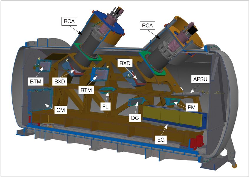
This page was intentionally left blank
Doc:                         ESO-331895
                                                             Issue:                          Issue 2.3.3
ESO          ESPRESSO Pipeline User Manual
                                                             Date:                     Date 2021-05-05
                                                             Page:                               3 of 73

                                           Change record
Issue/Rev.       Date      Section/Parag. affected         Reason/Initiation/Documents/Remarks
1.0           10/12/2018   all                       First public release,pipeline version 1.1.0
1.0.2         25/03/2019   all                       release update
1.2.3         24/05/2019   3                         Minor documentation updates
1.3.2         31/07/2019   all                       Updated, restructured, simplified, clarified
2.0.0         18/11/2020   all                       Updated, restructured, simplified, clarified
2.2.1         28/05/2021   all                       Updated
2.3.0         03/03/2021   -                         Description van-Dokkum cosmic rejection
2.3.3         05/05/2021   -                         CRH_MAP is now optional input of science recipe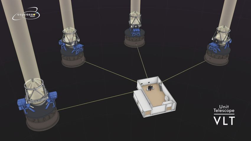
This page was intentionally left blank
Doc:                          ESO-331895
                                                                    Issue:                           Issue 2.3.3
    ESO           ESPRESSO Pipeline User Manual
                                                                    Date:                      Date 2021-05-05
                                                                    Page:                                5 of 73

Contents

1   Introduction                                                                                               11
    1.1   Purpose . . . . . . . . . . . . . . . . . . . . . . . . . . . . . . . . . . . . . . . . . . . . . . . 11
    1.2   Acknowledgments . . . . . . . . . . . . . . . . . . . . . . . . . . . . . . . . . . . . . . . . . 11
    1.3   Scope . . . . . . . . . . . . . . . . . . . . . . . . . . . . . . . . . . . . . . . . . . . . . . . . 11
    1.4   Reference documents . . . . . . . . . . . . . . . . . . . . . . . . . . . . . . . . . . . . . . . . 12

2   Overview                                                                                                   13

3   Recent improvements                                                                                        14

4   ESPRESSO Instrument Description                                                                            15
    4.1   Instrument overview . . . . . . . . . . . . . . . . . . . . . . . . . . . . . . . . . . . . . . . . 15
          4.1.1    Instrument description . . . . . . . . . . . . . . . . . . . . . . . . . . . . . . . . . . . 15
          4.1.2    The Coudé Trains . . . . . . . . . . . . . . . . . . . . . . . . . . . . . . . . . . . . . . 16
          4.1.3    The Front Ends . . . . . . . . . . . . . . . . . . . . . . . . . . . . . . . . . . . . . . . 16
          4.1.4    The Spectrograph . . . . . . . . . . . . . . . . . . . . . . . . . . . . . . . . . . . . . . 18
    4.2   Detector layout . . . . . . . . . . . . . . . . . . . . . . . . . . . . . . . . . . . . . . . . . . . 19

5   Known problems                                                                                             20

6   Instrument Data Description                                                                                22
    6.1   BIAS frames . . . . . . . . . . . . . . . . . . . . . . . . . . . . . . . . . . . . . . . . . . . . 23
    6.2   DARK frames . . . . . . . . . . . . . . . . . . . . . . . . . . . . . . . . . . . . . . . . . . . . 23
    6.3   Detector Flat-field (LED) frames . . . . . . . . . . . . . . . . . . . . . . . . . . . . . . . . . . 23
    6.4   ORDERDEF frames . . . . . . . . . . . . . . . . . . . . . . . . . . . . . . . . . . . . . . . . 23
    6.5   FLAT frames . . . . . . . . . . . . . . . . . . . . . . . . . . . . . . . . . . . . . . . . . . . . 23
    6.6   Wavelength calibration frames . . . . . . . . . . . . . . . . . . . . . . . . . . . . . . . . . . . 24
    6.7   Contamination by simultaneous reference frames . . . . . . . . . . . . . . . . . . . . . . . . . 24
    6.8   Fiber-to-fiber Relative Efficiency frames . . . . . . . . . . . . . . . . . . . . . . . . . . . . . . 24
    6.9   Spectrophotometric Calibration (FLUX) frames . . . . . . . . . . . . . . . . . . . . . . . . . . 24
    6.10 SCIENCE frames . . . . . . . . . . . . . . . . . . . . . . . . . . . . . . . . . . . . . . . . . . 24
Doc:                          ESO-331895
                                                                     Issue:                           Issue 2.3.3
    ESO           ESPRESSO Pipeline User Manual
                                                                     Date:                      Date 2021-05-05
                                                                     Page:                                6 of 73

7   Static Calibration Data                                                                                     25
    7.1   CCD Geometry Table . . . . . . . . . . . . . . . . . . . . . . . . . . . . . . . . . . . . . . . . 25
    7.2   Instrument Configuration Table . . . . . . . . . . . . . . . . . . . . . . . . . . . . . . . . . . . 25
    7.3   Led Flat Field gain windows Table . . . . . . . . . . . . . . . . . . . . . . . . . . . . . . . . . 25
    7.4   Wavelength Matrix Images . . . . . . . . . . . . . . . . . . . . . . . . . . . . . . . . . . . . . 25
    7.5   DLL Matrix Images . . . . . . . . . . . . . . . . . . . . . . . . . . . . . . . . . . . . . . . . . 26
    7.6   THAR line tables . . . . . . . . . . . . . . . . . . . . . . . . . . . . . . . . . . . . . . . . . . 26
    7.7   Flux Standard Star tables . . . . . . . . . . . . . . . . . . . . . . . . . . . . . . . . . . . . . . 26
    7.8   Extinction Table . . . . . . . . . . . . . . . . . . . . . . . . . . . . . . . . . . . . . . . . . . . 26
    7.9   Flux Template Table . . . . . . . . . . . . . . . . . . . . . . . . . . . . . . . . . . . . . . . . 26
    7.10 CCF Template Tables . . . . . . . . . . . . . . . . . . . . . . . . . . . . . . . . . . . . . . . . 27

8   Data Reduction                                                                                              28

9   Pipeline Recipes Interfaces                                                                                 31
    9.1   espdr_mbias . . . . . . . . . . . . . . . . . . . . . . . . . . . . . . . . . . . . . . . . . . . . . 32
          9.1.1    Input . . . . . . . . . . . . . . . . . . . . . . . . . . . . . . . . . . . . . . . . . . . . 32
          9.1.2    Output . . . . . . . . . . . . . . . . . . . . . . . . . . . . . . . . . . . . . . . . . . . 32
          9.1.3    Quality control . . . . . . . . . . . . . . . . . . . . . . . . . . . . . . . . . . . . . . . 32
          9.1.4    Parameters . . . . . . . . . . . . . . . . . . . . . . . . . . . . . . . . . . . . . . . . . 33
    9.2   espdr_mdark . . . . . . . . . . . . . . . . . . . . . . . . . . . . . . . . . . . . . . . . . . . . 33
          9.2.1    Input . . . . . . . . . . . . . . . . . . . . . . . . . . . . . . . . . . . . . . . . . . . . 33
          9.2.2    Output . . . . . . . . . . . . . . . . . . . . . . . . . . . . . . . . . . . . . . . . . . . 33
          9.2.3    Quality control . . . . . . . . . . . . . . . . . . . . . . . . . . . . . . . . . . . . . . . 33
          9.2.4    Parameters . . . . . . . . . . . . . . . . . . . . . . . . . . . . . . . . . . . . . . . . . 34
    9.3   espdr_led_ff . . . . . . . . . . . . . . . . . . . . . . . . . . . . . . . . . . . . . . . . . . . . . 34
          9.3.1    Input . . . . . . . . . . . . . . . . . . . . . . . . . . . . . . . . . . . . . . . . . . . . 34
          9.3.2    Output . . . . . . . . . . . . . . . . . . . . . . . . . . . . . . . . . . . . . . . . . . . 34
          9.3.3    Quality control . . . . . . . . . . . . . . . . . . . . . . . . . . . . . . . . . . . . . . . 34
          9.3.4    Parameters . . . . . . . . . . . . . . . . . . . . . . . . . . . . . . . . . . . . . . . . . 35
    9.4   espdr_orderdef . . . . . . . . . . . . . . . . . . . . . . . . . . . . . . . . . . . . . . . . . . . 35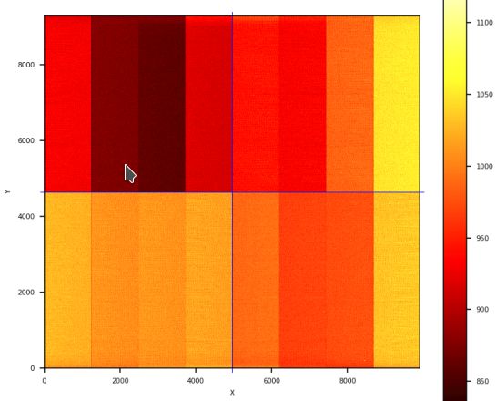
Doc:                          ESO-331895
                                                                 Issue:                           Issue 2.3.3
ESO           ESPRESSO Pipeline User Manual
                                                                 Date:                      Date 2021-05-05
                                                                 Page:                                7 of 73

      9.4.1    Input . . . . . . . . . . . . . . . . . . . . . . . . . . . . . . . . . . . . . . . . . . . . 35
      9.4.2    Output . . . . . . . . . . . . . . . . . . . . . . . . . . . . . . . . . . . . . . . . . . . 35
      9.4.3    Quality control . . . . . . . . . . . . . . . . . . . . . . . . . . . . . . . . . . . . . . . 35
      9.4.4    Parameters . . . . . . . . . . . . . . . . . . . . . . . . . . . . . . . . . . . . . . . . . 36
9.5   espdr_mflat . . . . . . . . . . . . . . . . . . . . . . . . . . . . . . . . . . . . . . . . . . . . . 36
      9.5.1    Input . . . . . . . . . . . . . . . . . . . . . . . . . . . . . . . . . . . . . . . . . . . . 36
      9.5.2    Output . . . . . . . . . . . . . . . . . . . . . . . . . . . . . . . . . . . . . . . . . . . 36
      9.5.3    Quality control . . . . . . . . . . . . . . . . . . . . . . . . . . . . . . . . . . . . . . . 36
      9.5.4    Parameters . . . . . . . . . . . . . . . . . . . . . . . . . . . . . . . . . . . . . . . . . 37
9.6   espdr_wave_FP . . . . . . . . . . . . . . . . . . . . . . . . . . . . . . . . . . . . . . . . . . . 37
      9.6.1    Input . . . . . . . . . . . . . . . . . . . . . . . . . . . . . . . . . . . . . . . . . . . . 37
      9.6.2    Output . . . . . . . . . . . . . . . . . . . . . . . . . . . . . . . . . . . . . . . . . . . 37
      9.6.3    Quality control . . . . . . . . . . . . . . . . . . . . . . . . . . . . . . . . . . . . . . . 38
      9.6.4    Parameters . . . . . . . . . . . . . . . . . . . . . . . . . . . . . . . . . . . . . . . . . 38
9.7   espdr_wave_THAR . . . . . . . . . . . . . . . . . . . . . . . . . . . . . . . . . . . . . . . . . 38
      9.7.1    Input . . . . . . . . . . . . . . . . . . . . . . . . . . . . . . . . . . . . . . . . . . . . 38
      9.7.2    Output . . . . . . . . . . . . . . . . . . . . . . . . . . . . . . . . . . . . . . . . . . . 39
      9.7.3    Quality control . . . . . . . . . . . . . . . . . . . . . . . . . . . . . . . . . . . . . . . 39
      9.7.4    Parameters . . . . . . . . . . . . . . . . . . . . . . . . . . . . . . . . . . . . . . . . . 40
9.8   espdr_wave_LFC . . . . . . . . . . . . . . . . . . . . . . . . . . . . . . . . . . . . . . . . . . 40
      9.8.1    Input . . . . . . . . . . . . . . . . . . . . . . . . . . . . . . . . . . . . . . . . . . . . 40
      9.8.2    Output . . . . . . . . . . . . . . . . . . . . . . . . . . . . . . . . . . . . . . . . . . . 40
      9.8.3    Quality control . . . . . . . . . . . . . . . . . . . . . . . . . . . . . . . . . . . . . . . 41
      9.8.4    Parameters . . . . . . . . . . . . . . . . . . . . . . . . . . . . . . . . . . . . . . . . . 41
9.9   espdr_cal_contam . . . . . . . . . . . . . . . . . . . . . . . . . . . . . . . . . . . . . . . . . . 41
      9.9.1    Input . . . . . . . . . . . . . . . . . . . . . . . . . . . . . . . . . . . . . . . . . . . . 41
      9.9.2    Output . . . . . . . . . . . . . . . . . . . . . . . . . . . . . . . . . . . . . . . . . . . 42
      9.9.3    Quality control . . . . . . . . . . . . . . . . . . . . . . . . . . . . . . . . . . . . . . . 42
      9.9.4    Parameters . . . . . . . . . . . . . . . . . . . . . . . . . . . . . . . . . . . . . . . . . 42
9.10 espdr_cal_eff_ab . . . . . . . . . . . . . . . . . . . . . . . . . . . . . . . . . . . . . . . . . . 42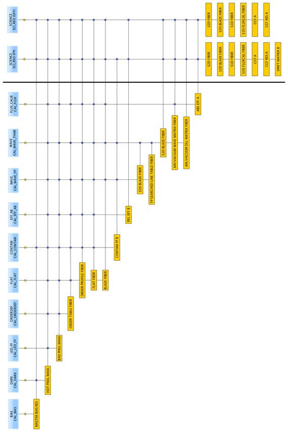
Doc:                           ESO-331895
                                                                Issue:                            Issue 2.3.3
ESO         ESPRESSO Pipeline User Manual
                                                                Date:                       Date 2021-05-05
                                                                Page:                                 8 of 73

      9.10.1 Input . . . . . . . . . . . . . . . . . . . . . . . . . . . . . . . . . . . . . . . . . . . . 42
      9.10.2 Output . . . . . . . . . . . . . . . . . . . . . . . . . . . . . . . . . . . . . . . . . . . 43
      9.10.3 Quality control . . . . . . . . . . . . . . . . . . . . . . . . . . . . . . . . . . . . . . . 43
      9.10.4 Parameters . . . . . . . . . . . . . . . . . . . . . . . . . . . . . . . . . . . . . . . . . 43
9.11 espdr_cal_flux . . . . . . . . . . . . . . . . . . . . . . . . . . . . . . . . . . . . . . . . . . . . 44
      9.11.1 Input . . . . . . . . . . . . . . . . . . . . . . . . . . . . . . . . . . . . . . . . . . . . 44
      9.11.2 Output . . . . . . . . . . . . . . . . . . . . . . . . . . . . . . . . . . . . . . . . . . . 44
      9.11.3 Quality control . . . . . . . . . . . . . . . . . . . . . . . . . . . . . . . . . . . . . . . 44
      9.11.4 Parameters . . . . . . . . . . . . . . . . . . . . . . . . . . . . . . . . . . . . . . . . . 45
9.12 espdr_sci_red . . . . . . . . . . . . . . . . . . . . . . . . . . . . . . . . . . . . . . . . . . . . 45
      9.12.1 Input . . . . . . . . . . . . . . . . . . . . . . . . . . . . . . . . . . . . . . . . . . . . 45
      9.12.2 Output for OBJ_F P        . . . . . . . . . . . . . . . . . . . . . . . . . . . . . . . . . . . 46
      9.12.3 Output for OBJ_SKY         . . . . . . . . . . . . . . . . . . . . . . . . . . . . . . . . . . 47
      9.12.4 Quality control . . . . . . . . . . . . . . . . . . . . . . . . . . . . . . . . . . . . . . . 47
      9.12.5 Parameters . . . . . . . . . . . . . . . . . . . . . . . . . . . . . . . . . . . . . . . . . 48
9.13 espdr_compu_drift . . . . . . . . . . . . . . . . . . . . . . . . . . . . . . . . . . . . . . . . . 49
      9.13.1 Input . . . . . . . . . . . . . . . . . . . . . . . . . . . . . . . . . . . . . . . . . . . . 49
      9.13.2 Output . . . . . . . . . . . . . . . . . . . . . . . . . . . . . . . . . . . . . . . . . . . 49
      9.13.3 Quality control . . . . . . . . . . . . . . . . . . . . . . . . . . . . . . . . . . . . . . . 50
      9.13.4 Parameters . . . . . . . . . . . . . . . . . . . . . . . . . . . . . . . . . . . . . . . . . 50
      9.13.5 Example . . . . . . . . . . . . . . . . . . . . . . . . . . . . . . . . . . . . . . . . . . 50
9.14 espdr_wave_THAR_THAR . . . . . . . . . . . . . . . . . . . . . . . . . . . . . . . . . . . . . 51
      9.14.1 Input . . . . . . . . . . . . . . . . . . . . . . . . . . . . . . . . . . . . . . . . . . . . 51
      9.14.2 Output . . . . . . . . . . . . . . . . . . . . . . . . . . . . . . . . . . . . . . . . . . . 51
      9.14.3 Quality control . . . . . . . . . . . . . . . . . . . . . . . . . . . . . . . . . . . . . . . 51
      9.14.4 Parameters . . . . . . . . . . . . . . . . . . . . . . . . . . . . . . . . . . . . . . . . . 51
9.15 espdr_wave_LFC_LFC . . . . . . . . . . . . . . . . . . . . . . . . . . . . . . . . . . . . . . . 51
      9.15.1 Input . . . . . . . . . . . . . . . . . . . . . . . . . . . . . . . . . . . . . . . . . . . . 52
      9.15.2 Output . . . . . . . . . . . . . . . . . . . . . . . . . . . . . . . . . . . . . . . . . . . 52
      9.15.3 Quality control . . . . . . . . . . . . . . . . . . . . . . . . . . . . . . . . . . . . . . . 52
      9.15.4 Parameters . . . . . . . . . . . . . . . . . . . . . . . . . . . . . . . . . . . . . . . . . 52
Doc: ESO-331895
Issue: Issue 2.3.3
ESO ESPRESSO Pipeline User Manual
Date: Date 2021-05-05
Page: 9 of 73
10 Quick start 53
10.1 ESPRESSO pipeline recipes . . . . . . . . . . . . . . . . . . . . . . . . . . . . . . . . . . . . 53
10.2 An introduction to Reflex and EsoRex . . . . . . . . . . . . . . . . . . . . . . . . . . . . . . . 53
10.2.1 Using Reflex . . . . . . . . . . . . . . . . . . . . . . . . . . . . . . . . . . . . . . . . 54
10.3 Quick Start: Reducing The Demo Data . . . . . . . . . . . . . . . . . . . . . . . . . . . . . . 54
10.3.1 Using EsoRex . . . . . . . . . . . . . . . . . . . . . . . . . . . . . . . . . . . . . . . . 58
11 Algorithms and recipe details 60
11.1 Algorithms . . . . . . . . . . . . . . . . . . . . . . . . . . . . . . . . . . . . . . . . . . . . . 60
11.1.1 Master frame combination using a kappa-sigma-clipped mean/median . . . . . . . . . . 60
11.1.2 Order definition . . . . . . . . . . . . . . . . . . . . . . . . . . . . . . . . . . . . . . . 60
11.1.3 Background subtraction . . . . . . . . . . . . . . . . . . . . . . . . . . . . . . . . . . 60
11.1.4 Spectrum Extraction . . . . . . . . . . . . . . . . . . . . . . . . . . . . . . . . . . . . 61
11.1.5 Flat-Fielding . . . . . . . . . . . . . . . . . . . . . . . . . . . . . . . . . . . . . . . . 61
11.1.6 Wavelength Calibration . . . . . . . . . . . . . . . . . . . . . . . . . . . . . . . . . . . 62
11.1.7 Instrumental Drift Measurement . . . . . . . . . . . . . . . . . . . . . . . . . . . . . . 62
11.1.8 Sky Subtraction . . . . . . . . . . . . . . . . . . . . . . . . . . . . . . . . . . . . . . . 63
11.1.9 Barycentric Correction . . . . . . . . . . . . . . . . . . . . . . . . . . . . . . . . . . . 63
11.1.10 Order Rebinning and Merging . . . . . . . . . . . . . . . . . . . . . . . . . . . . . . . 64
11.1.11 Radial Velocity Computation . . . . . . . . . . . . . . . . . . . . . . . . . . . . . . . . 65
11.1.12 Removal of cosmic rays . . . . . . . . . . . . . . . . . . . . . . . . . . . . . . . . . . 65
11.1.13 Error and Bad Pixel Propagation . . . . . . . . . . . . . . . . . . . . . . . . . . . . . . 66
11.2 Recipes . . . . . . . . . . . . . . . . . . . . . . . . . . . . . . . . . . . . . . . . . . . . . . . 67
11.2.1 mbias . . . . . . . . . . . . . . . . . . . . . . . . . . . . . . . . . . . . . . . . . . . . 67
11.2.2 mdark . . . . . . . . . . . . . . . . . . . . . . . . . . . . . . . . . . . . . . . . . . . . 67
11.2.3 led_ff . . . . . . . . . . . . . . . . . . . . . . . . . . . . . . . . . . . . . . . . . . . . 67
11.2.4 orderdef . . . . . . . . . . . . . . . . . . . . . . . . . . . . . . . . . . . . . . . . . . . 67
11.2.5 mflat . . . . . . . . . . . . . . . . . . . . . . . . . . . . . . . . . . . . . . . . . . . . 68
11.2.6 cal_contam . . . . . . . . . . . . . . . . . . . . . . . . . . . . . . . . . . . . . . . . . 68
11.2.7 cal_eff_ab . . . . . . . . . . . . . . . . . . . . . . . . . . . . . . . . . . . . . . . . . . 68
11.2.8 wave_FP . . . . . . . . . . . . . . . . . . . . . . . . . . . . . . . . . . . . . . . . . . 69Doc: ESO-331895
Issue: Issue 2.3.3
ESO ESPRESSO Pipeline User Manual
Date: Date 2021-05-05
Page: 10 of 73
11.2.9 wave_THAR . . . . . . . . . . . . . . . . . . . . . . . . . . . . . . . . . . . . . . . . 69
11.2.10 wave_LFC . . . . . . . . . . . . . . . . . . . . . . . . . . . . . . . . . . . . . . . . . 69
11.2.11 cal_flux . . . . . . . . . . . . . . . . . . . . . . . . . . . . . . . . . . . . . . . . . . . 70
11.2.12 sci_red . . . . . . . . . . . . . . . . . . . . . . . . . . . . . . . . . . . . . . . . . . . 70
11.2.13 compu_drift . . . . . . . . . . . . . . . . . . . . . . . . . . . . . . . . . . . . . . . . . 71
11.2.14 wave_THAR_THAR . . . . . . . . . . . . . . . . . . . . . . . . . . . . . . . . . . . . 71
11.2.15 wave_LFC_LFC . . . . . . . . . . . . . . . . . . . . . . . . . . . . . . . . . . . . . . 71
A Installation 72
A.1 System Requirements . . . . . . . . . . . . . . . . . . . . . . . . . . . . . . . . . . . . . . . . 72
A.2 Installing the Pipeline KIT . . . . . . . . . . . . . . . . . . . . . . . . . . . . . . . . . . . . . 72
A.3 Installing the Software including ESOReflex . . . . . . . . . . . . . . . . . . . . . . . . . . . . 73Doc: ESO-331895
Issue: Issue 2.3.3
ESO ESPRESSO Pipeline User Manual
Date: Date 2021-05-05
Page: 11 of 73
1 Introduction
1.1 Purpose
The ESPRESSO pipeline is a subsystem of the VLT Data Flow System (DFS). Its target user is both the user
community and ESO Data Products Department (DPD) in the generation of master calibration data, in the re-
duction of scientific exposures, and in the data quality control. It should also serve as a quick look tool for
Paranal Science Operations (PSO). Additionally, the ESPRESSO pipeline recipes are made public to the user
community, to allow a more personalised processing of the data from the instrument. The ESPRESSO pipeline
was developed with the declared objective of providing precise Radial Velocity (RV) data and accurate wave-
length calibration. The purpose of this document is to describe a typical ESPRESSO data reduction sequence
with the ESPRESSO pipeline.
This manual is a complete description of the data reduction recipes implemented by the the ESPRESSO pipeline,
reflecting the status of the ESPRESSO pipeline as of May 05, 2021 (version 2.3.3).
1.2 Acknowledgments
The ESPRESSO pipeline has been designed, implemented and developed by the Geneva Observatory. We are
particularly grateful to the responsibles for the data reduction: Christophe Lovis, Danuta Sownowska and Alex
Segovia for their contributions and support.
Andrea Modigliani, from ESO, provided the Reflex workflow, DFS support and most of the documentation. We
thank also Pedro Figueira, Andrea Mehner and Richard Anderson for providing useful feedback to improve the
reflex workflow and documentation.
1.3 Scope
This document describes the ESPRESSO pipeline used at ESO-Garching and ESO-Paranal for the purpose of
data assessment and data quality control.
Updated versions of the present document may be found on [1]. For general information about the current
instrument pipelines status we remind the user of [2]. Quality control information are at [3].
Additional information on the Common Pipeline Library (CPL) and ESOREX can be found respectively at
[4], [5]. A description of the instrument is in [6]. The ESPRESSO instrument user manual is in [7]. The
ESPRESSO Reflex tutorial is in [8].Doc: ESO-331895
Issue: Issue 2.3.3
ESO ESPRESSO Pipeline User Manual
Date: Date 2021-05-05
Page: 12 of 73
1.4 Reference documents
[1] ESPRESSO Pipeline Users’ Manual VLT-MAN-ESO-19500-XXXX
www.eso.org/pipelines
[2] Current pipeline status
www.eso.org/observing/dfo/quality/pipeline-status.html
[3] ESO-Data Flow Operation home page http://www.eso.org/observing/dfo/quality/
[4] CPL home page www.eso.org/cpl
[5] ESOREX home page www.eso.org/cpl/esorex.html
[6] ESPRESSO home page
www.eso.org/sci/facilities/paranal/instruments/espresso
[7] VLT ESPRESSO User Manual VLT-MAN-ESO-14700-3517
www.eso.org/sci/facilities/paranal/instruments/espresso/doc
[8] Reflex ESPRESSO Tutorial www.eso.org/pipelinesDoc: ESO-331895
Issue: Issue 2.3.3
ESO ESPRESSO Pipeline User Manual
Date: Date 2021-05-05
Page: 13 of 73
2 Overview
In collaboration with instrument consortia, the Pipeline Systems Department (PSD) of the Software Develope-
ment Division is implementing data reduction pipelines for the most commonly used VLT/VLTI instrument
modes. These data reduction pipelines have three main purposes:
Data quality control: pipelines are used to produce the quantitative information necessary to monitor instru-
ment performance.
Master calibration product creation: pipelines are used to produce master calibration products (e.g., com-
bined bias frames, super-flats, wavelength dispersion solutions).
Science product creation: using pipeline-generated master calibration products, science products are produced
for the supported instrument modes (e.g., combined ISAAC jitter stacks; bias-corrected, flat-fielded FORS
images, wavelength-calibrated UVES spectra). The accuracy of the science products is limited by the
quality of the available master calibration products and by the algorithmic implementation of the pipelines
themselves. In particular, adopted automatic reduction strategies may not be suitable or optimal for all
scientific goals.
Instrument pipelines consist of a set of data processing modules that can be called from the command line, from
the automatic data management tools available on Paranal or from Gasgano.
ESO offers two front-end applications for launching pipeline recipes, Gasgano and EsoRex [5] both included
in the pipeline distribution (see Appendix A, page 72). These applications can also be downloaded separately
from www.eso.org/gasgano and www.eso.org/cpl/esorex.html. GASGANO is a Data File
Organiser developed and maintained by ESO to help its user community to manage and organise in a systematic
way the astronomical data observed and produced by all VLT compliant telescopes, i.e. by telescopes which are
being operated through Observation Blocks. The tool also supports FITS files which are not generated by those
telescopes with limited functionality. For further information, please, refer to the latest Gasgano User’s
Manual. In the special case of the ESPRESSO pipeline, which uses a lot of RAM, we decided not to provide
Gasgano support.
Recent pipeline improvements are listed in Section 3. The ESPRESSO instrument is described in Section 4.
In section 5 we list known data reduction problems for the ESPRESSO pipeline and possible solutions. The
different types of ESPRESSO raw frames and auxilliary data are described in Sections 6, and 7. An overview
of the data reduction, the input data, and the recipes involved in the calibration cascade is provided in section
8. More details on inputs, products, quality control measured quantities, and controlling parameters of each
recipe is given in section 9. A brief introduction to the usage of the available reduction recipes using EsoRex
is presented in Section 10. More detailed descriptions of the data reduction algorithms used by the individual
pipeline recipes can be found in Section 11.
In Appendix A the installation of the ESPRESSO pipeline recipes is described.Doc: ESO-331895
Issue: Issue 2.3.3
ESO ESPRESSO Pipeline User Manual
Date: Date 2021-05-05
Page: 14 of 73
3 Recent improvements
This release of the ESPRESSO pipeline (version 2.3.3) includes the following major improvements with respect
to public release: 2.2.1
• Updated order tracing recipe to use the inter-order background measurement for orders tracing. This
enable a more robust order tracing for high binned (e.g. H42) settings.
• Adjusted parameters in the inst_config of HR42 to improve the robustness of HR42 processing.
• Fix a few minor typos found in the FITS header of science recipe products in Phase III format.
• Updated extraction routine to handle cosmics detected by van-Dokkum method and simplified extraction
algorithm (no more interpolation of hot/bad pixels).
• Fixed some problems in the update of plots shown in the science reflex interactive workflow.Doc: ESO-331895
Issue: Issue 2.3.3
ESO ESPRESSO Pipeline User Manual
Date: Date 2021-05-05
Page: 15 of 73
4 ESPRESSO Instrument Description
ESPRESSO is the Echelle SPectrograph for Rocky Exoplanets and Stable Spectroscopic Observations installed
at the incoherent combined Coudé facility of the VLT. It is an ultra-stable fibre-fed échelle high-resolution
spectrograph which collects the light from either a single UT or the four UTs simultaneously via the so-called
UT Coudé trains. The whole system is built to reach the ultimate radial-velocity precision of 10 cm/s over a
timespan of 10 years in single UT mode.
In this chapter a brief description of the ESPRESSO instrument is given. A more complete documentation can
be found in the ESPRESSO User Manual, downloadable from
www.eso.org/sci/facilities/paranal/instruments/espresso.
4.1 Instrument overview
ESPRESSO is the ESO/VLT high-resolution spectrograph designed to measure precise radial velocities on a
long timespan with the main scientific aim of detecting and characterising Earth mass exoplanets in the habitable
zone of solar-like stars.
ESPRESSO is a highly-stabilized fibre-fed échelle spectrograph that can be fed with light from either a single or
the four Unit Telescopes (UTs) simultaneously. The instrument is installed at the incoherent combined Coudé
focus (ICCF) of the VLT. The light from an astronomical source is redirected from the telescopes to the detectors
through three components of the ICCF facility: the UT Coudé trains, the front end units, and the spectrograph
itself. The Coudé Trains (CT) bring the light from each telescope to the Combined Coudé Lab (CCL) through
11 optical elements, including mirrors, lenses, and prisms. The four Front Ends (one for each UT) receive the
light from the CTs and feed the spectrograph entrance fibres. The Fibre Link transports the light from the Front
Ends to the vacuum vessel. The latter is thermally stabilized at the mK level and stabilized in pressure down to
the µbar. The light is then going through the optical components of the spectrograph and split up into a red and
a blue spectrum which are recorded on the corresponding science detectors.
The spectrograph is fed by two fibres, one for the target and the other one for simultaneous calibration (either
the sky or a simultaneous reference: Fabry-Pérot, Laser Frequency Comb, or Thorium-Argon lamp). The light
from the two fibres is recorded onto a blue (380-525nm) and a red (525-788nm) CCD mosaic. ESPRESSO
can operate in three main instrument configurations: High Resolution 1-UT (HR), Ultra High-Resolution 1-UT
(UHR) and Medium Resolution 4-UT (MR). The main characteristics of these modes are summarised in Table
4.1.0.
4.1.1 Instrument description
ESPRESSO is the first instrument of a VLT facility that can host instrumentation at the so-called Incoherent
Combined Coudé Focus (ICCF). As such, in order to describe the instrument, one needs to understand the three
components through which the light travels from the telescope to the detectors. These are: the UT Coudé Trains,
the Front Ends, and the Spectrograph itself. Each of these components are described below. For a more detailed
description, we point the interested reader to the ESPRESSO user manual.Doc: ESO-331895
Issue: Issue 2.3.3
ESO ESPRESSO Pipeline User Manual
Date: Date 2021-05-05
Page: 16 of 73
Table 4.1.0: EXPRESSO specifications
HR(1-UT) UHR(1-UT) MR(4-UT)
Wavelength range 380-788 nm 380-788 nm 380-788 nm
Resolving power (median) 140,000 190,000 70,000
Aperture on sky 100 .0 000 .5 4x100 .0
Total peak efficiency 11% 6% 11%
RV precision (requirement) < 10 cm/s < 5 m/s < 5 m/s
Limiting V-band magnitude ≈ 17 ≈ 16 ≈20
Binning 1x1, 2x1 1x1 4x2, 8x4
Spectral sampling (average) 4.5 px 2.5 px 5.5 px (binned x2)
Spectral sampling per slice 9.0(4.5) px 5.0 px 5.5 px (binned x4)
Number of slices 2 2 1 (merged)
Detector read-out mode FAST (1x1), FAST SLOW
SLOW (2x1)
CCD pixel binning 1x1 and 2x1 1x1 4x2 and 8x4
RON (blue detector) 8e-/pix 8e-/pix 3e-/pix
RON (red detector) 5e-/pix 5e-/pix 2e-/pix
CONAD 1.1e-/ADU 1.1e-/ADU 1.1e-/ADU
4.1.2 The Coudé Trains
Distances between each UT and the Combined Coudé Laboratory (CCL) range between 48 m for UT2 and 69
m for UT1. A trade-off analysis between solutions based on mirrors, prisms, lenses, and fibres, points towards
a full-optics solution. The chosen design with the position of the 11 optical elements is shown below in the
second figure. The Coudé train picks up the light through a prism at the level of the Nasmyth-B platform and
routes the beam through the UT mechanical structure down to the UT Coudé room, and farther to the CCL along
the existing incoherent light ducts. The four trains relay a field of 17 arcsec around the acquired object to the
CCL. The selected concept to convey the light of the telescope from the Nasmyth-B focus to the entrance of
the tunnel in the Coudé room (CR) below each UT is based on a set of 6 prisms (with some power). The light
is directed from the UT’s Coudé room towards the CCL using 2 large lenses. The beams from the four UTs
meet in the CCL, where mode selection and beam conditioning is performed by the fore-optics of the Front-End
sub-system.
4.1.3 The Front Ends
The Front-End transports the beam received from the Coudé, once corrected for atmospheric dispersion by
the ADC, to the common focal plane where the pickups for the spectrograph fiber feeds are located. While
performing such a beam conditioning, the Front-End can apply pupil and field stabilizations. These are achieved
via two independent control loops each composed of a technical camera and a tip-tilt stage. Another dedicated
stage delivers a focusing function. In addition, the Front-End handles the injection of the calibration light,
prepared in the Calibration Unit, into the fibers and then into the spectrograph. As wavelength calibration
sources, ESPRESSO is equiped with a laser frequency comb (LFC), two ThAr lamps and a Fabry Perot Etalon
system for simultaneous measurement of the radial velocity (RV) drift. A toggling mechanism handles theDoc: ESO-331895
Issue: Issue 2.3.3
ESO ESPRESSO Pipeline User Manual
Date: Date 2021-05-05
Page: 17 of 73
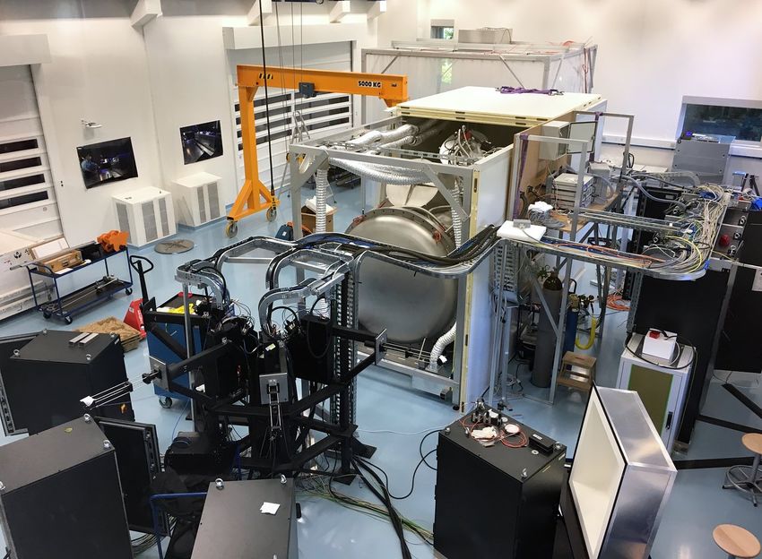
Figure 4.1.1: An view of ESPRESSO
Figure 4.1.2: An view of Coudé Trains (left) and of the front end unit (right).
selection between the possible observing modes in a passive way.
Link sub-system relays the light from the Front-End to the spectrograph and forms the spectrograph pseudo-slit
inside the vacuum vessel. The 1-UT mode uses two octagonal fibres each, one for the object and one for the sky
or simultaneous reference. In the high-resolution (singleHR) mode, the fibre has a core of 140 µm, equivalent
to 1 arcsec on the sky; in the ultra-high resolution (singleUHR) mode, the fibre core is 70 µm and the covered
field of view is 0.5 arcsec. The fibre entrances are organized in pickup heads that are moved to the focal plane
of the Front End when the specific bundle of the specific mode is selected. In the 4-UT mode (multiMR), four
object fibres and four sky/reference fibres are fed simultaneously by the four telescopes. The four object fibres
will finally feed a single square 280 µm object fibre, while the four sky/reference fibres will feed a single square
280 µm sky/reference fibre. In the 4-UT mode, the spectrograph will see a pseudo: the four individual fibres
are bundled together and fed into a square fiber, that is then imaged by the instrument leading to a single square
image on the detector. Another essential task performed by the Fibre-link sub-system is the light scrambling.
The use of a double-scrambling optical system will ensure both scrambling of the near field and far field of the
light beam. A high scrambling gain, which is crucial to obtain the required RV precision in the 1-UT mode is
achieved by the use of octagonal fibres (Chazelas et al. 2011).Doc: ESO-331895
Issue: Issue 2.3.3
ESO ESPRESSO Pipeline User Manual
Date: Date 2021-05-05
Page: 18 of 73
4.1.4 The Spectrograph
The spectrograph optics are mounted in a 3-dimensional optical bench specifically designed to keep the optical
system within the thermo-mechanical tolerances required for high-precision radial velocity measurements. The
bench is mounted in a vacuum vessel in which 10-3 mbar class vacuum is maintained during the entire duty cycle
of the instrument. The temperature at the level of the optical system is required to be stable at the mK level in
order to avoid both short-term drift and long-term mechanical instabilities. Such an ambitious requirement is
obtained by locating the spectrograph in a multi-shell active thermal enclosure system. Each shell improves the
temperature stability by a factor of 10, thus getting from typically Kelvin-level variations in the CCL down to 1
mK stability inside the vacuum vessel and on the optical bench.
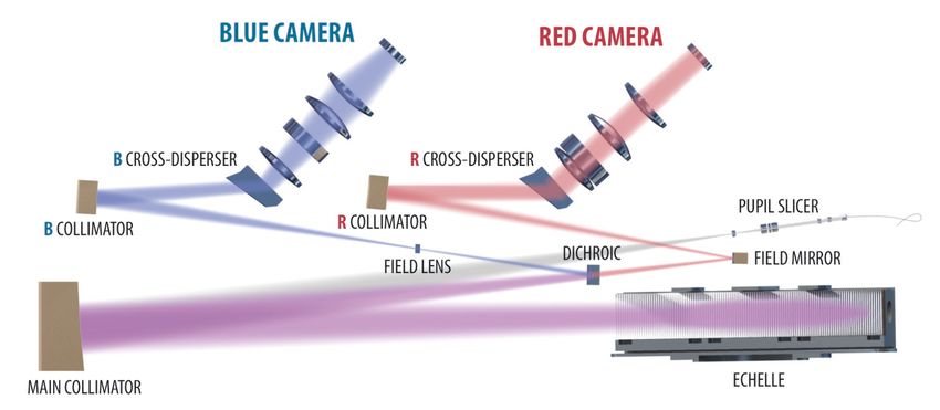
At the entrance of the spectrograph, an anamorphic pupil slicing unit (APSU) shapes the beam in order to
compress the beam in cross-dispersion direction but not in main-dispersion direction, where high resolving
power needs to be achieved. In the latter direction, however, the pupil is sliced and superimposed on the echelle
grating to minimize its size. The rectangular white-pupil is then re-imaged and compressed by the anamorphic
VPH grism. Given the wide spectral range and the required efficiency, two large 90x90 mm CCD detectors are
required to record the full spectrum. Therefore, a dichroic beam splitter separates the beam in a blue and a red
channel which in turn allows to optimize each spectroscopic arm for image quality and optical efficiency. Each
of the two blue and red cross-dispersers has the function of separating the dispersed spectrum in all its spectral
orders. In addition, an anamorphism is re-introduced to make the pupil square and to compress the order width
in cross-dispersion direction, such that the inter-order space is maximized.
Figure 4.1.3: ESPRESSO: opto-mechanical path (left) and optical path (right).Doc: ESO-331895
Issue: Issue 2.3.3
ESO ESPRESSO Pipeline User Manual
Date: Date 2021-05-05
Page: 19 of 73
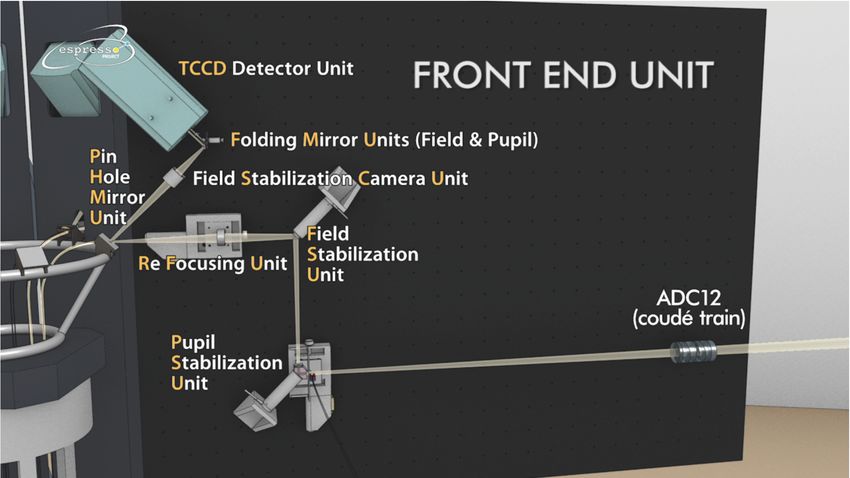
4.2 Detector layout
ESPRESSO data include two images, one for each camera, that are stored in two extensions of a FITS files. The
detector geometry is described in the following image.
Figure 4.2.1: ESPRESSO master bias (left) and detailed geometry of the read-out regions (right). As shown in
the image each detector has 16 read-out regions each with a different bias level.Doc: ESO-331895
Issue: Issue 2.3.3
ESO ESPRESSO Pipeline User Manual
Date: Date 2021-05-05
Page: 20 of 73
5 Known problems
Several pipeline problems have been identified:
• Slow execution time.The data reduction chain in SINGLE mode may take around 45min on a regular
computer (RAM=16 GB).
The code parallelisation with OpenMP does enable faster reduction on multi-core platforms. The speed
improves significantly if data and reduction is done on very fast I/O disks, like SSDs, and processors with
high clock speed.
• Failure of THAR-FP or FP-THAR reduction The reduction of THAR-FP or FP-THAR fails sometime,
when the espdr_wave_FP recipe does not detect FP peaks on the whole order. This can be due to a
strong cosmic, badly placed. The consequence is the impossibility to construct the wavelength solution.
In this case it is possible to take another FP-FP raw frame for the reduction.
• Cosmic rays in raw calibrations. There have been reported few cases in which the science pipeline
crashes with no apparent reason, providing the following error message:
10:00:07 [WARNING] espdr_correct_flux: [tid=000] ESC[31mFlux correction not performed:
no flux template available for spectral type F5ESC[0m
10:00:07 [ INFO ] : [tid=000] Computing CCF for fibre A sky_sub for size_y = 170 ...
10:00:47 [ ERROR ] espdr_sci_red: [tid=000] espdr_compute_CCF failed for sky_sub:
Access beyond boundaries
10:00:47 [ ERROR ] cpl_errorstate_dump: [tid=000] Lost 11192 CPL error(s)
10:00:47 [ ERROR ] cpl_errorstate_dump_one_level: [tid=000] [11193/11212]
’Access beyond boundaries’ (11) at cpl_image_get:cpl_image_io.c:747
To our best knowledge, the problem is associated to the presence of cosmic rays on some raw calibrations
(category: WAVE,FP,FP), which led to a product that caused the failure in the science recipe. Future
versions of the pipeline will be able to identify such issues and flag them appropriately.
To overcome the issue, two solutions are currently available:
– Remove the cosmic ray from the faulty calibrations with external tools before starting the data
reduction.
– Replace the calibrations with those from a previous or following day. It might be worth replacing all
the calibrations (all WAVE, ORDERDEF, and FLAT types), even if not all are affected by cosmic
rays, to avoid fibre misalignment between calibrations from different days.
• Interference pattern introduced by the Coude Train ESPRESSO spectra are affected by two different
interference patterns induced by coude train optics. Aproximately sinusoidal “wiggles” become apparent
when spectra taken in different telescope positions are divided by each other. The first set of wiggles has
a period of 30 Åat 600 nm and an amplitude of ∼ 1%). In contrast, the second set of wiggles has a shorter
period of 1 Åat 600 nm and an amplitude of ∼ 0.1 %. For further information the user is referred to Allart
et al. 2020. The consortium and ESO are working together to characterize this effect.
• wave_FP fails Occasionally WAVE,FP,FP frames may have cosmics that may induce a recipe failure. For
example we encounter this problem and the reported error was like the following:Doc: ESO-331895
Issue: Issue 2.3.3
ESO ESPRESSO Pipeline User Manual
Date: Date 2021-05-05
Page: 21 of 73
[ INFO ] espdr_wave_FP: Checking FP peaks for fibre A
[WARNING] espdr_wave_FP: Delta x bigger for order 92 pxl 297.402747, delta = 5
[WARNING] espdr_wave_FP: Peak_pxls: 291.580109, 297.402747, 309.016369
[ ERROR ] espdr_wave_FP: Missing peaks in the FP image, aborting.
[ ERROR ] espdr_wave_FP: Dumping all 1 error(s):
[ ERROR ] espdr_wave_FP: [1/1] ’Input data do not match’ (13) at espdr_wave_
[ ERROR ] esorex: Execution of recipe ’espdr_wave_FP’ failed, status = 13
[ INFO ] esorex: Calculating product checksums
[WARNING] esorex: Writing of output sof omitted due to previous errors
Already the warning indicates something suspicious happen. Often the source of the problem is one or
more cosmic on the frame. Often this problem can be solved during extraction simply by reducing the
parameter fp_extraction_ksigma from the default 5 to a smaller value.
For updated information we recommend the user to also read the Data Reduction F.A.Q. page: http://www.eso.org/sci/data-
processing/faq.html.Doc: ESO-331895
Issue: Issue 2.3.3
ESO ESPRESSO Pipeline User Manual
Date: Date 2021-05-05
Page: 22 of 73
6 Instrument Data Description
The ESPRESSO instrument produces raw data in five different configurations or modes. Those are defined by
the main instrument mode and detector binning. The corresponding FITS keywords are:
• HIERARCH ESO INS MODE: instrument mode, defining the fiber head used and the spectral resolution
and sampling.
• HIERARCH ESO DET BINX: detector binning in cross-dispersion direction (also called spatial direction)
• HIERARCH ESO DET BINY: detector binning in main dispersion direction
The five available configurations are:
• SINGLEHR mode and 1x1 binning (HR11)
• SINGLEHR mode and 2x1 binning (HR21)
• SINGLEUHR mode and 1x1 binning (UHR)
• MULTIMR mode and 4x2 binning (MR42)
• MULTIMR mode and 8x4 binning (MR84)
The ESPRESSO pipeline considers these five configurations as independent instruments for the purpose of data
reduction. This means that, to be processed by the pipeline a science frame in a given configuration requires
a complete calibration dataset in the same configuration. As part of the ESPRESSO operational scheme at the
observatory, the acquisition of the required calibration frames is automatically triggered based on the science
data obtained during the night and the need for instrument monitoring.
To reduce a science frame, the following raw calibration frames are needed:
type # frames comments
BIAS 10 to determine RON, bias level, residuals
DARK 5 long exposure time (>20min), to determine hot pixels
LED 2x5 2 different exposure times, to determine non linear pixels and convertion factor
ORDERDEF 2 each frame illuminates only one fiber, to trace orders
FLAT 2x10 2 sets, illuminating fib A and B,
to determine short and long scale responsiveness variations
FP-FP 1 both fibres illuminated by Fabry Perot etalon, for wavelength calibration
Thorium-FP 1 fib A illuminated by ThAr, fibre B by FP, for wavelength calibration
FP-Thorium 1 fib B illuminated by ThAr, fibre A by FP, for wavelength calibration
SKY,SKY 1 both fibres observing zenith sky, to determine relative fibre efficiency
STD,SKY 1 fib A observes a spectrophotometric standard, fib B observes the sky
to flux calibrate the observed science spectrumDoc: ESO-331895
Issue: Issue 2.3.3
ESO ESPRESSO Pipeline User Manual
Date: Date 2021-05-05
Page: 23 of 73
Optionally, the following calibration frames are needed for wavelength calibration with the laser frequency
comb (LFC):
type # frames comments
LFC-FP 1 for wavelength calibration, optional
FP-LFC 1 for wavelength calibration, optional
Optionally, the following calibration frame is needed to correct for cross-fiber contamination by the FP in
simultaneous-reference mode:
type # frames comments
DARK-FP 1 frame to determine contamination of fib B on A
It is also necessary to have a set of static calibration data (see next Section).
The following sections provides a brief description of each raw data type involved in the data reduction chain.
6.1 BIAS frames
Bias frames are zero exposure frames taken to measure the readout noise, the mean bias level, and fixed-pattern
structure in the bias level for each read-out port (refer to Figure 4.2.1 for an example of bias detector image).
6.2 DARK frames
Dark frames are taken to measure the detector dark current and identify hot pixels. A set of five input frames is
acquired, each with an exposure time of 3600s.
6.3 Detector Flat-field (LED) frames
Detector flat-field frames are images taken while illuminating the detector with a uniform LED light. At least
two sets, each composed by at least five frames, with different exposure times are required.
6.4 ORDERDEF frames
Two frames are acquired: ORDERDEF_A and ORDERDEF_B and used for order/slice definition, identification
and tracing for fibre A and B. A continuum light source is used to illuminate fibre A (or B), while fibre B (or A)
is dark (separate frames for different fibres are necessary for the automatic identification of orders or slices).
6.5 FLAT frames
Two set of frames are acquired: FLAT_A and FLAT_B and used to derive the order profile in cross-dispersion
direction, the spectral flat-field, and the blaze function of the spectrograph for fibres A and B. A continuum lightDoc: ESO-331895
Issue: Issue 2.3.3
ESO ESPRESSO Pipeline User Manual
Date: Date 2021-05-05
Page: 24 of 73
source is used to illuminate fibre A (or fibre B), while fibre B (or fibre A) is dark. Several exposures (at least
10) are required to reach sufficiently high SNR.
6.6 Wavelength calibration frames
Three sets of frames are acquired to perform the wavelength calibration. These are acquired with different
calibration sources and combined together to cross-calibrate the wavelength references of the two fibres.
• FP_FP: This frame is obtained illuminating both fibres with a Fabry Perot.
• THAR_FP: This frame is obtained illuminating fibre A with a ThAr lamp and fibre B with a Fabry Perot.
• FP_THAR: This frame is obtained illuminating fibre B with a ThAr lamp and fibre A with a Fabry Perot.
• LFC_FP (optional): This frame is obtained illuminating fibre A with a laser comb and fibre A with a
Fabry Perot.
• FP_LFC (optional): This frame is obtained illuminating fibre B with a laser comb and fibre A with a
Fabry Perot.
6.7 Contamination by simultaneous reference frames
• CONTAM_FP: Measurement of contamination light induced on fibre A by FP simultaneous reference on
fibre B. Fibre A is dark, while FP light is injected into fibre B as in a science exposure with simultaneous
reference (i.e. same flux level).
6.8 Fiber-to-fiber Relative Efficiency frames
EFF_AB: Relative efficiency of fibre B vs. fibre A as a function of wavelength. During twilight, the telescope
is pointed at zenith and the skylight is injected into both fibres.
6.9 Spectrophotometric Calibration (FLUX) frames
FLUX_CALIB: A spectrophotometric standard star is observed, as in a science exposure, with sky.
6.10 SCIENCE frames
The following frames are acquired:
• SCIENCE_FP: Science exposure (target on fibre A) with Fabry-Perot simultaneous reference on fibre B.
• SCIENCE_SKY: Science exposure (target on fibre A) with simultaneous sky on fibre B.Doc: ESO-331895
Issue: Issue 2.3.3
ESO ESPRESSO Pipeline User Manual
Date: Date 2021-05-05
Page: 25 of 73
7 Static Calibration Data
In the following section static calibration (called also ancillary) data required for ESPRESSO data reduction are
listed. Static calibration data correspond to Images or Tables describing configuration setups, reference data,
or characteristics of the instrument that are considered to be fixed. This sets them apart from the calibration
previously described. For each of them we indicate the corresponding value of the HIERARCH ESO PRO
CATG, in short its PRO.CATG, which has to be used to identify the frames listed in the Set of Frames (see
Section 10.3.1, page 58).
7.1 CCD Geometry Table
These are the static CCD configuration tables describing the CCD geometry. The table contains the number and
sizes of the detectors, outputs and prescan and overscan regions. There is one table for each of the supported
detector binnigs. Its PRO.CATG is CCD_GEOM.
7.2 Instrument Configuration Table
These are the static instrument configuration tables providing the pipeline recipes with all necessary input pa-
rameters that are intimately linked to the instrument configuration being used. There will be one such table per
instrument mode (i.e. five for ESPRESSO) and period of validity. Its PRO.CATG is INST_CONFIG.
7.3 Led Flat Field gain windows Table
These static tables indicate for each detector and detector read-out region the windows where the conver-
sion factor is computed. There is one table for each of the supported detector binnings. Their PRO.CATG
is LED_FF_GAIN_WINDOWS.
7.4 Wavelength Matrix Images
These are the wavelength calibration arrays (one per fibre) in S2D format, with the wavelength of each extracted
pixel stored as data value. These are used as static input frames in the flat and wavelength (THAR/FP or
FP/THAR) data reduction. Their PRO.CATG is STATIC_WAVE_MATRIX_A/B1 .
1
As static WAVE and DLL matrix frames, have a large size, to reduce the size of the pipeline package, we decided to include them
in the demo data, available http://www.eso.org/sci/software/pipelines/, and to deliver them to the user together with
the raw data when retrieved with the calSelector tool. The FITS filename of the frame delivered with the demo data contains the
instrument mode, the binning, the corresponding PRO.CATG and fibre information and a date that correspond to the date since the
frame is valid. Raw data should be associated with the closest in time static frame, which is the default behavior in case of Reflex based
data reduction.Doc: ESO-331895
Issue: Issue 2.3.3
ESO ESPRESSO Pipeline User Manual
Date: Date 2021-05-05
Page: 26 of 73
7.5 DLL Matrix Images
These are the pixel widths in wavelength calibration arrays (one per fibre) in S2D format, with the width in
wavelength of each extracted pixel stored as data value. These are used as static input frames in the wavelength
(THAR/FP or FP/THAR) and science data reduction. Their PRO.CATG is STATIC_DLL_MATRIX_A/B2 .
7.6 THAR line tables
These are the static ThAr line tables (one per fibre) containing the wavelengths, approximate positions, flux
and values of D - the FP mirrors distance, for the emission lines found in the ThAr extracted spectra (S2D).
The column called "grouping" is used to save the mode of the corresponding FP peak. The table is not ex-
pected to change over the lifetime of the instrument owing to the high long-term stability of ESPRESSO. Their
PRO.CATG is REF_LINE_TABLE_A/B.
7.7 Flux Standard Star tables
The Flux Standard Star Table lists all the stars (part of the calibration plan) for which we have a precise physical
flux calibration [ergs/s/cm2 /A] on an even wavelength scale. The table contains absolute spectral energy distri-
butions of a sample of spectrophotometric standard stars. It is a required input of the recipe espdr_cal_flux
during response and efficiency estimation, where the observed photometric standard star spectrum, after proper
rescaling by exposure time, gain and atmospheric extinction, is divided by the spectrum of the corresponding
standard star from this catalog. Its PRO.CATG is STD_TABLE.
7.8 Extinction Table
This is the table containing the atmospheric extinction curve for Paranal, as provided in Patat et al. (2011), A&A
527, 91 (their Appendix B). This is used in the espdr_cal_flux to determine the efficiency and instrument
response and in the espdr_sci_red, to flux calibrate the observed science object spectrum. Its PRO.CATG
is EXT_TABLE.
7.9 Flux Template Table
This is the table containing observed spectral energy distributions of a sample of reference stars with different
spectral types spanning late-F to early-M. Suitable stars are solar-metallicity dwarf stars of spectral types F to
M, observed at high SNR and at low airmass. To build the flux template, the S2D flux of the star is summed in
each spectral order and normalised to one at an arbitrary wavelength (e.g. 550 nm). The flux template is simply
the integrated normalised flux in each spectral order. Flux Template table corresponds to the flux distribution as
a function of wavelength for stars of different spectral types. This primordial flux is used to correct the effect
of chromatic extinction of the atmosphere, composed of several factors, like Rayleight scattering and ozone +
aerosols absorption. Its PRO.CATG is FLUX_TEMPLATE.
2
DLL stands for Delta LL, a short notation corresponding to Delta Wavelength.Doc: ESO-331895
Issue: Issue 2.3.3
ESO ESPRESSO Pipeline User Manual
Date: Date 2021-05-05
Page: 27 of 73
7.10 CCF Template Tables
The template tables, or CCF masks, are used by the cross-correlation process. They consist of a list of rest
(RV=0) wavelengths for the spectral lines of interest, along with their relative depth (contrast) with respect to
the continuum. Depths are used as weights in the CCF process since Doppler precision is proportional to line
depth. Their PRO.CATG are MASK_TABLE.
These CCF masks are created from actual ESPRESSO spectra of stars covering a range of sub-spectral types.
Spectral lines are identified through an automatic procedure and included in the mask if they meet a number of
criteria such as large enough depth and limited blending. The current pipeline version includes CCF masks for
all M dwarfs down to M6 (individual fits files). The masks cover the full wavelength range of ESPRESSO.Doc: ESO-331895
Issue: Issue 2.3.3
ESO ESPRESSO Pipeline User Manual
Date: Date 2021-05-05
Page: 28 of 73
8 Data Reduction
We give below an overview of the global reduction cascade, starting from basic calibrations down to science
reduction. The ESPRESSO association map is shown in Figure 8.0.0.
• Detector bias level and readout noise are measured on stacked BIAS frames (master bias). The stacking
is used to remove the cosmics. In ESPRESSO the mean bias level and readout noise in any raw frame are
best obtained from the overscan regions. The master bias is thus not used as such in the reduction cascade.
A master bias residual frame is generated by the espdr_mbias recipe by subtracting the overscan from
the master bias. It is used instead to subtract the fixed residual bias level structure across detector outputs.
The residual bias level pattern is not negligible for low-SNR science exposures.
• DARK frames are used to measure the average detector dark current and identify the hot pixels. The
master dark frame is generated via stacking and sigma-clipping to remove the cosmics. The mean dark
current level per output and the hot pixels are computed on the master dark frame and stored in the hot
pixel mask. The hot pixels are obtained through the sigma-clipping applied on the master image of each
detector output.
• Detector flat-field frames are acquired to characterise unresponsive (“dead”) pixels or pixels with a very
different gain (so called: bad pixels). For each exposure time, a set of minimum five LED_FF frames
is needed to remove the cosmics via the sigma clipping on the pixel-by-pixel basis. The bad pixel mask
is obtained from the analysis of master LED_FF frames taken with different exposure times (linearity
check). The conversion factor is measured for each detector output from the relation between flux level
and standard deviation of pixel values. It is stored in the bad pixel mask.
• ORDERDEF frames (one per fibre) are used to identify and trace spectral orders or slices on the detector.
Each order or slice is fitted in the cross-dospersion direction, with a gaussian every defined number of
pixels. The gaussians peaks are fitted with a low degree polynomial, of which coefficients are saved in
the recipe products.
• For each fibre, the order profile in cross-dispersion direction is found using high-SNR, co-added FLAT
frames. Then, the orders are extracted from the FLAT frames using this profile, and the spectral flat-field
is generated. The (extracted) blaze function is obtained through smoothing of the FLAT spectra and cor-
rection for the spectral energy distribution of the calibration lamp. The order extraction assumes that 1)
main-dispersion direction runs approximately parallel to CCD rows/columns, and 2) slit image tilt is close
to zero with respect to CCD columns/rows. In this case, order extraction becomes extremely simple and
does not require wavelength calibration frames to track different positions along the slit. The ESPRESSO
optical design makes this strategy possible (line tilt very close to zero), and even recommended owing to
its simplicity. This method has been successfully applied to HARPS and other radial-velocity spectro-
graphs.
• CONTAM frames are used to measure cross-fibre contamination on fibre A from the simultaneous refer-
ence on fibre B (ThAr lamp, laser comb or Fabry-Perot). Contamination frames are used during extraction
in the science reduction.
• The relative efficiency of channels A and B as a function of wavelength is measured using EFF_AB
frames, which are obtained through blue sky observations. The obtained relative efficiency is used toDoc: ESO-331895
Issue: Issue 2.3.3
ESO ESPRESSO Pipeline User Manual
Date: Date 2021-05-05
Page: 29 of 73
scale the subtraction on science exposures with simultaneous sky. Even though these are called fibre-to-
fibre relative efficiency they, de facto, calibrate the whole Coude train as seen through fibre A and B. As
such, they are UT dependent.
• The wavelength calibration for both fibres is determined using WAVE frames. It is done in two steps: first
with the Fabry-Perot on both fibres and then with one of the fibres illuminated by ThAr lamp. In addition
the wavelength solution can be computed using frames with Laser Frequency Comb. Since the LFC does
not cover the whole spectral range, the THAR-FP solution is needed to complete the calibration products.
On fibre A (science fibre), the wavelength solution is particularly important since it is used to calibrate the
science spectrum and therefore sets the radial velocity zero point. On fibre B, the simultaneously acquired
spectrum mainly serves as reference to calculate the drift on science frames that use FP as simultaneous
reference.
• FLUX_CALIB frames are used to compute the absolute efficiency of the instrument as a function of
wavelength, using spectrophotometric standard stars. The efficiency is computed from the comparison
between the observed spectrum and reference flux table.The efficiency curve is used in the science re-
duction to calibrate the science spectrum in flux. The precision of the flux calibration is generally low
because of highly variable fibre losses due to seeing.
• Finally, SCIENCE frames are of two different sub-types depending on the source of light on the fibre B:
sky or Fabry-Perot. Science reduction makes use of all calibration products listed above and generates
extracted S2D spectra and merged, rebinned S1D spectra, together with S2D and S1D error and quality
maps. Finally, the cross-correlation function (CCF) of the S2D spectrum is computed and the radial
velocity is obtained from a Gaussian fit to the CCF.Doc: ESO-331895
Issue: Issue 2.3.3
ESO ESPRESSO Pipeline User Manual
Date: Date 2021-05-05
Page: 30 of 73
Figure 8.0.0: The cascade of the ESPRESSO pipeline recipes. For the calibration recipes, only the products
used later in the reduction chain are listed. The science recipes have all the products listed.Doc: ESO-331895
Issue: Issue 2.3.3
ESO ESPRESSO Pipeline User Manual
Date: Date 2021-05-05
Page: 31 of 73
9 Pipeline Recipes Interfaces
In this section we provide for each recipe 3 examples of the required input data (and their tags). In the following
we assume that /path_file_raw/filename_raw.fits and /path_file_cdb/filename_cdb.fits are existing FITS files.
We also provide a list of the pipeline products for each recipe, indicating their default recipe name, the value of
the FITS keyword HIERARCH ESO PRO CATG (in short PRO.CATG) and a short description.
The relevant keywords used to classify each frame are the following:
Association keyword Information
HIERARCH ESO DPR TYPE data type
HIERARCH ESO INS MODE mode
HIERARCH ESO DET BINX detector bin X
HIERARCH ESO DET BINY detector bin Y
HIERARCH ESO PRO CATG product category
For each recipe we list in a table the input parameters (as they appear in the recipe configuration file), the
corresponding aliases (the corresponding names to be eventually set on command line) and their default values.
Also quality control parameters are listed. Those are stored in relevant pipeline products. More information on
instrument quality control can be found on www.eso.org/qc. ESPRESSO spectral format data of the BLUE
and RED camera are stored in two image extensions.
The user may obtain brief description of the main input recipe parameters by typing
esorex -help recipe,
for example,
esorex -help espdr_mbias
A possible esorex configuration parameter value is –suppress-prefix=FALSE, in which case all products will be
renamed with a prefix settable by the parameter –output-prefix, defaulted to out_, and an increasing number,
like (out_0000.fits, out_0001.fits, out_000N.fits) For this reason the table briefly describing
the products contains also a first column indicating the product ID, which is the value of the product number
(with minimum significant digits).
The pipeline performs several quality assesment on the data. The result is stored in a QC keyword that has value
“QC CHECK”, where the indicates the kind of check done. A check is successful if
the value of the keyword is 1. Some recipe may do several tests. It is also created a keyword “QC
CHECK”, where indicates the recipe executed, that indicates the overall product of all checks.
The PRO.CATG chosen for the extracted spectra falls into two groups: ’S2D_*’ spectra, that can be of type A
or B to represent the object or the calibration fibersi, respectively. These files are 2D images where the rows
(Y axis) contain the extracted spectrum of a given order or slice. We remind the reader that in order to keep
compact the spectrograph the input light beam from the input slices is split in two slices. These are dispersed
by the grating and imaged on the detectors (one for each instrument arm) on different orders. As the input beam
3
We do not describe here two recipes: the recipe espdr_single_bias, used to reduce HARPS data, and the recipe es-
pdr_wave_TH_drift, used for the wavelength calibration when are not available enough good quality FP, FP frames.Doc: ESO-331895
Issue: Issue 2.3.3
ESO ESPRESSO Pipeline User Manual
Date: Date 2021-05-05
Page: 32 of 73
is sliced in two component the order shows two components, adjacent one to another. These order slices are
distinguishible in UHR and HR modes and overlap in the MR mode. There are 45 orders in the Blue and 40 in
the red. In UHR and HR modes the pipeline extracts then two slices for each order, and in MR only one.
9.1 espdr_mbias
9.1.1 Input
type TAG n setting
raw BIAS 5...n any
ref CCD_GEOM 1 match
ref INST_CONFIG 1 match
9.1.2 Output
ID PRO.CATG type Note
0 MASTER_BIAS qc Master bias
1 MASTER_BIAS_RES cdb Master bias residuals
9.1.3 Quality control
This recipe computes the following QC parameters (on the image extension n, and read-out region i,j):
QC key name description
QC EXTn ROXi ROYj BIAS RON read out noise [ADU].
QC EXTn ROXi ROYj BIAS RON EL read out noise [e-]
QC EXTn ROXi ROYj OVSC RON read out noise on overscan region [ADU]
QC EXTn ROXi ROYj OVSC RON EL read out noise on overscan region [e-]
QC BIAS RON CHECK quality check on RON computation
QC EXTn ROXi ROYj BIAS MEAN mean bias [ADU]
QC EXTn ROXi ROYj BIAS MEAN EL mean value [e-]
QC EXTn ROXi ROYj BIAS STRUCTX X structure
QC EXTn ROXi ROYj BIAS STRUCTY Y structure
QC EXTn ROXi ROYj RES MEAN mean value of residuals [ADU]
QC EXTn ROXi ROYj RES MEAN EL mean value of residuals [e-]
QC EXTn ROXi ROYj RES STDEV rms of residuals [ADU]
QC EXTn ROXi ROYj RES STDEV EL rms of residuals [e-]
QC EXTn ROXi ROYj RES TEST quality check on residual computation on read-out region n
QC RES TEST overall quality check on residual computation
QC BIAS OUTLIERS number out utliers on bias
QC OVSC OUTLIERS number of outliers on region
QC BIAS MEAN CHECK quality check on bias mean computation
QC BIAS CHECK overall quality check assessmentYou can also read