Value of Rehabilitation Training for Children with Cerebral Palsy Diagnosed and Analyzed by Computed Tomography Imaging Information Features under ...
←
→
Page content transcription
If your browser does not render page correctly, please read the page content below
Hindawi
Journal of Healthcare Engineering
Volume 2021, Article ID 6472440, 9 pages
https://doi.org/10.1155/2021/6472440

Research Article
Value of Rehabilitation Training for Children with Cerebral Palsy
Diagnosed and Analyzed by Computed Tomography Imaging
Information Features under Deep Learning

          Xi Zhang ,1 Zhenfang Wang ,1 Jun Liu ,2 Lulin Bi ,3 Weilan Yan ,1
          and Yueyue Yan 1
          1
            Department of Rehabilitation, Children’s Hospital of Shanxi Province, Taiyuan 030025, Shanxi, China
          2
            Outpatient Department of Infectious Diseases, Children’s Hospital of Shanxi Province, Taiyuan 030025, Shanxi, China
          3
            Imaging Department of CT Room, Children’s Hospital of Shanxi Province, Taiyuan 030025, Shanxi, China

          Correspondence should be addressed to Zhenfang Wang; lyt@zjnu.edu.cn

          Received 26 May 2021; Revised 30 June 2021; Accepted 12 July 2021; Published 21 July 2021

          Academic Editor: Enas Abdulhay

          Copyright © 2021 Xi Zhang et al. This is an open access article distributed under the Creative Commons Attribution License,
          which permits unrestricted use, distribution, and reproduction in any medium, provided the original work is properly cited.

          To analyze the brain CT imaging data of children with cerebral palsy (CP), deep learning-based electronic computed tomography
          (CT) imaging information characteristics were used, thereby providing help for the rehabilitation analysis of children with CP and
          comorbid epilepsy. The brain CT imaging data of 73 children with CP were collected, who were outpatients or inpatients in our
          hospital. The images were randomly divided into two groups. One group was the artificial intelligence image group, and hybrid
          segmentation network (HSN) model was employed to analyze brain images to help the treatment. The other group was the control
          group, and original images were used to help diagnosis and treatment. The deep learning-based HSN was used to segment the CT
          image of the head of patients and was compared with other CNN methods. It was found that HSN had the highest Dice score
          (DSC) among all models. After treatment, six cases in the artificial intelligence image group returned to normal (20.7%), and the
          artificial intelligence image group was significantly higher than the control group (X2 � 335191, P < 0.001). The cerebral he-
          modynamic changes were obviously different in the two groups of children before and after treatment. The VP of the cerebral
          artery in the child was (139.68 ± 15.66) cm/s after treatment, which was significantly faster than (131.84 ± 15.93) cm/s before
          treatment, P < 0.05. To sum up, the deep learning model can effectively segment the CP area, which can measure and assist the
          diagnosis of future clinical cases of children with CP. It can also improve medical efficiency and accurately identify the patient’s
          focus area, which had great application potential in helping to identify the rehabilitation training results of children with CP.

1. Introduction                                                         rescue technology, more and more ultrapremature babies
                                                                        are able to survive. These premature babies are extremely
Cerebral palsy (CP) is one of the common causes of disability           immature and face severe challenge such as breathing,
in children. It is the brain tissue damage caused by the                nutrition, metabolism, and infection. Their brain damage
immature brain (fetal period to within one year of life) due            easily occurs, CP is caused, and the risk of disability is in-
to congenital malformations or hypoxia, trauma, infection,              creased [2, 3]. Neuroimaging examination is an important
and other factors after birth, which further causes a group of          auxiliary examination for central nervous system damage,
neurological syndromes in children with nonprogressive                  which can provide objective basis for changes in tissue
movement abnormalities and postural abnormalities as the                morphology for clinical diagnosis and treatment. The tra-
main manifestations, accompanied by cognition, sensory,                 ditional cranial CT has been widely used in the cranial
and communication disorders and other complications [1].                imaging examination of children with CP and has accu-
With the continuous development of perinatal medicine and               mulated certain experience [4]. The other functional im-
neonatal life support technology and the improvement of                 aging examinations developed based on traditional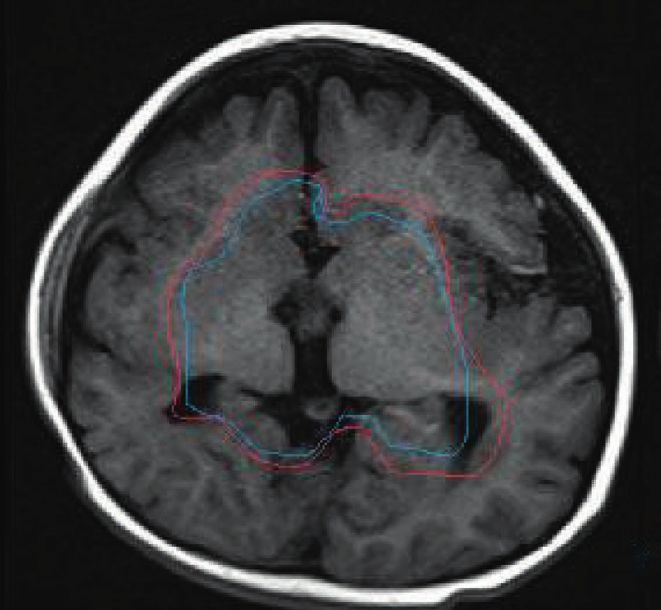
2                                                                                           Journal of Healthcare Engineering

techniques such as magnetic resonance imaging (MRI),             analysis has gradually become a research hotspot in the
ultrasound (US), positron emission tomography (PET), and         medical field. Artificial intelligence algorithms have been
other devices can assess the function of brain tissue through    used in the field of medical image data analysis and pro-
local blood flow changes, water molecular activity, and           cessing. By integrating these algorithms into clinical prac-
metabolic status. The lesions associated with the occurrence     tice, effective and accurate diagnostic results are obtained.
of CP were mapped in more detail to provide evidence of          The traditional method of intelligent imaging diagnosis
functional and metabolic abnormalities for some lesions          compares the automatically labeled or segmented area with
with insignificant morphological changes. Up to now,              the predefined benchmark template, but it still needs the
medical imaging is an indispensable part of the clinic, and it   imaging expert to give the final diagnosis result. In the ap-
plays an irreplaceable role in diagnosis and treatment.          plication of disease diagnosis, abdominal CT imaging is the
However, the workload of doctors is huge. Studies showed         most important imaging means in the clinical diagnosis and
that, in some cases, general radiologists must make a di-        follow-up of tumor diseases, which is widely used in the
agnosis every three to four seconds in an 8-hour working day     detection, segmentation, and diagnosis of lesions. Since dif-
to meet the needs of the workload [5]. The accuracy of           ferent types of lesions correspond to different characteristics,
doctors’ diagnosis results will be greatly affected by such a     how to separate the lesion area from the image is the key to the
large work intensity, and misdiagnosis and missed diagnosis      success of the high-precision diagnosis system [10]. To im-
will be caused. However, there are also obvious problems in      prove the accuracy of the automatic diagnosis system, the
the current study. (I) The commonly used brain images have       medical image assisted diagnosis system based on artificial
millimeter resolution. However, some diseases do not cause       intelligence mainly includes four aspects as follows: (I) image
significant structural changes and require high resolution        preprocessing, which improves the image quality and en-
and small-scale brain imaging techniques. (II) The sample        hances the contrast of lesions; (II) detection and segmentation
data only contains a certain kind of special diseases and        of the region of interest (ROI), which reduces the influence of
health data. In actual diagnosis, the patient may suffer from     interference background on the system; (III) feature extrac-
ten related diseases. (III) The excessive number of extracted    tion, selection, and classification, which improve the char-
features consumes a large amount of storage space and at the     acterization ability of the target; (IV) the semantic
same time greatly increases the computational complexity         segmentation of tumor, which can obtain the semantic fea-
and leads to dimensional disaster. (IV) The classification        tures of lesions and improve the accuracy of recognition. The
accuracy should be further improved to meet the require-         extraction of efficient features in the four key steps of the
ments of practical use. (V) The generalization performance       auxiliary diagnosis system is the core technology of the
of the classifier is poor, and the prediction effect of the new    system. At present, the performance of medical image aided
samples is obviously lower than that of the training samples.    diagnosis system based on shallow learning completely de-
    With the development of artificial intelligence (AI),         pends on the characterization ability of features and the
people began to try to use computer technology to assist         generalization performance of classification diagnosis model.
doctors in diagnosis, which produced a computer-aided                In short, the development of AI technology has provided
diagnosis (CAD) [6]. Taking the most widely used mam-            new ideas to solve such medical problems. In particular,
mography CAD screening as an example, more than 74% of           multidisciplinary knowledge such as radiology and com-
mammograms in the United States were performed with the          puter science was integrated by imaging omics. High-
aid of the CAD system by 2010 [7]. However, the advantages       throughput features can be mined from medical images and
of CAD were questionable; several large trials concluded that    modeled and analyzed to provide clinical decision support
there was little benefit from CAD. The accuracy of radiol-        for rehabilitation training for children with CP.
ogists’ diagnoses was reduced; thus high biopsy rates were
caused. To eliminate the false alarms generated by these         2. Methods
systems, the diagnostic process becomes more complex [8].
At present, diagnosis based on medical imaging mainly relies     2.1. Research Object. Children with CP who were outpatient or
on radiologists’ manual review of images and manual              hospitalized in our hospital from June 2017 to June 2020 were
analysis of radiological images. This is a very time-con-        taken as research subjects. A total of 73 cases met the re-
suming work, requiring radiologists to consult hundreds of       quirements; 44 were males and 29 were females. The age range
sections and multiple lesions through three-dimensional CT       was 1 to 14 years and the average age was 47.7 ± 37.2 months.
scanning equipment [9]. For early detection, detecting le-            The classification was carried out according to the gross
sions that are “too small to characterize” is particularly       motor function classification system (GMFCS) [11]. There
important, which requires time and effort on the part of the      were 8 cases of GMFCS I (4 males, 4 females), 21 cases of
radiologist. In addition, the increasing huge amount of          GMFCS II (12 males, 9 females), 23 cases of GMFCS III (13
image data also brings great challenges for image reading. To    males, 10 females), 11 cases of GMFCS IV (8 males, 3 females),
effectively improve the efficiency of medical image reading,        and 10 cases of GMFCS V (7 males, 3 females).
reduce the error rate of diagnosis, and provide effective
auxiliary information for imaging physicians, the auxiliary
diagnostic technology based on intelligent image analysis is     2.1.1. Inclusion Criteria. The abovementioned children met
becoming more and more important. In recent years,               the diagnostic criteria for CP and must meet the following
computer-aided diagnosis based on intelligent image              four necessary conditions: (a) nonprogressive aggravating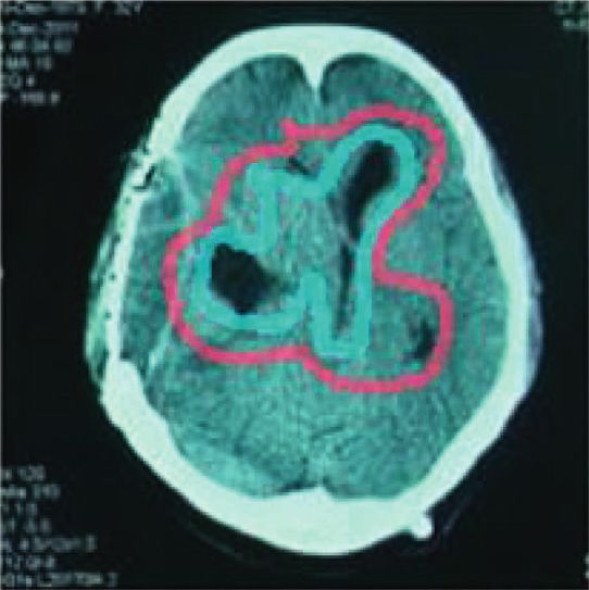
Journal of Healthcare Engineering                                                                                               3

dysfunction that persisted, which was caused by central            To reduce the size of the feature map, the step S3D con-
nervous system damage; children with complications such as         volution was used to replace the pooling operation. The goal
muscle damage and joint deformation as the course of CP            of the decoder was generating high resolution feature maps.
was prolonged; (b) children with deviations in motor de-           First, the feature graph was upsampled, and then the
velopment and abnormal postures (motor development was             upsampled feature graph was cascaded with the feature
included or not included); (c) the original reflex not dis-         graph from the corresponding level of the encoder. After
appearing or the erection reflex and balance response               cascading, the MSC module was used to adjust the number
delayed or absent, which may be accompanied by a positive          of feature graphs. The lightweight 3D CNN had fewer pa-
pathological reflex; (d) children with abnormal muscle tone         rameters and computational costs compared to the original
and strength. In addition, there were two reference condi-         3D U-NET.
tions whether it met the diagnosis of CP: (a) children with a
history or risk factors that cause CP; (b) children with cranial
imaging evidence.                                                  2.3.2. Deep Learning Mode. The Python deep learning
                                                                   framework was used to write code, which was trained on
                                                                   NVIDIA GeForce GTX 1080TIGPU. There were 100
2.1.2. Exclusion Criteria. The exclusion criteria included (a)     training cycles and the training time was about 12 hours. The
the diagnosis of abnormal motor development in children            Adam optimizer was used with an initial learning rate of
that was consistent with general developmental retardation         0.001. The GDL loss function similar to the previous chapter
and developmental coordination disorder; (b) children with         was used to optimize network parameters. If the validation
induced epileptic seizures caused by acute ketoacidosis,           set loss was not decreased in the last 20 training cycles, the
water and electrolyte disorders, acute brain injury, febrile       learning rate was reduced to 1/5 of the original. The rotation,
convulsions, hypoglycemia, and drug poisoning, etc.; (c)           scaling, deformation, mirroring, and other data were not
children with metal implants or other contraindications for        used to enhance technology to focus on the impact of
CT examination; (d) children with abnormal motor function          network structure. The LeakyReLU was used as the acti-
caused by other genetic metabolic reasons; (e) children with       vation function. The negative part of the feature information
motor dysfunction and epileptic seizures caused by tumors,         can be retained by LeakyReLU to prevent falling into a local
peripheral neuropathy, and genetic metabolic diseases, etc.        minimum compared with the standard ReLU. For 2D CNN,
    A total of 73 children with CP met the above inclusion         batch normalization was used to reduce internal covariant
criteria and were included in the research. The research had       offset problems. For 3D CNN, a number of criteria were
been approved by the medical ethics committee of X hos-            calculated using instance normalization as performance
pital, and the informed consent form had been signed by the        indicators to quantify the segmentation results, including
families of the children involved in the research.                 DSC, sensitivity, and positive predictive value (PPV).

2.2. Experimental Equipment. 74 contrast-enhanced CT               2.4. Comparative Test with 3DCNN Method. Compared with
samples constituted the dataset of the research. The Philips       the 3D CNN method, each CT was first resampled to
Brilliance 1281 CT scanner (Philips Healthcare, Amsterdam,         256 × 256 × 64 to maximize the utilization of 11 GB of GPU
Netherlands) was used. The tube voltage and current were           memory. In the decoder, each layer was composed of a
120 kV and 220 mA, respectively, the size of the collimator        trilinear upsampling layer with a factor of two, followed by
was 64 × 0.625 mm, and the Fov was 20 × 20 cm. The                 two 3 × 3 × 3 convolutions, and instance normalization and
512 × 512 size imaging matrix was used, the pixel size range       LeakyReLU were used to activate each layer. The jump
was 0.58 to 0.98 mm, and the reconstruction interval was           connection was used to provide the decoder with spatial
5 mm. All scans were manually segmented by two radiol-             information from the encoder. Finally, the nearest neighbor
ogists using Itk snap software (version 3.4; http://www.           sampling was used to upsample the segmentation result to
itksnap.org), and the segmentation differences were re-             the size of 512 × 512 × 64.
solved through discussion until a consensus was reached.
The data set was randomly divided into three subsets, and 84,
                                                                   2.5. Treatment Methods. The physical therapy (PT), occu-
20, and 30 samples were included for training, verification,
                                                                   pational therapy (OT), and speech therapy (ST) were used as
and testing, respectively.
                                                                   the main treatment methods. The selected method was
                                                                   Bobath’s method to suppress the abnormal posture, ab-
2.3. Experimental Environment                                      normal posture reflex, and abnormal movement patterns of
                                                                   children with CP. The facilitating techniques were used to
2.3.1. CNN Model. The proposed CNN model is shown in               promote cervical erection, sitting erection, standing erec-
Figure 1, which was similar to 3D U-NET. The image fea-            tion, and static and dynamic balance in children with CP.
tures can be extracted layer by layer by the encoder, and the      The German Voyt method was selected to perform reflex
segmentation map can be generated by the decoder. The 3D           movement of the body to promote normal motor devel-
U-Net was modified to be suitable for this task. In the             opment and induce training with reflex turning over and
original 3D U-Net, there were two 3 × 3 × 3 convolutions           reflex abdominal crawling. According to the child’s condi-
included in each level, which was replaced by two modules.         tion, one-to-one rehabilitation training was carried out by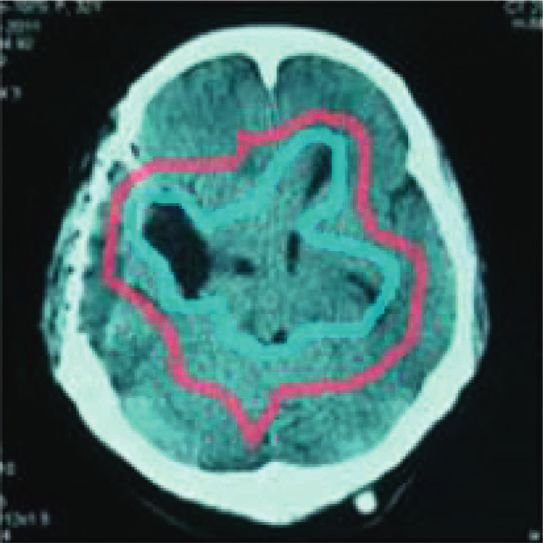
4                                                                                                Journal of Healthcare Engineering

                              NSC                                1×1×1
                                                                  conv
                                                                                           S3D conv

                          16 × 16 × 16

                                                                                                 16 × 16 × 16

                             32 × 16 × 16                                         32 × 16 × 16

                                                             126 × 16 × 16
                                                     Figure 1: CNN model.

the rehabilitation therapist. The training was one to two           compared, analysis of variance was carried out first, and then
hours a day, and 90 days was a course of treatment. The             pairwise comparison was made. Enumeration data were
rehabilitation training for children with mild CP was one to        expressed as percentage (%), and comparison between two
two courses, and the rehabilitation training for children with      groups was performed by χ 2 test or corrected χ 2 test. P < 0.05
severe CP was three to four courses.                                was considered statistically significant.
                                                                    3. Results
2.6. Observation Indicators. Before and after treatment, the
cerebral artery blood flow velocity (VP) and the vascular            3.1. Comparative Test with 2DCNN Method. It was compared
pulse index (PI) of the children in both groups were ex-            with 2D CNN method. The 2D models allowed larger images
amined by Libong CBC-II transcranial doppler (TCD) ce-              as input than 3D models (Figure 2). Therefore, full-reso-
rebrovascular ultrasound to understand the recovery of              lution CT slices were used to collect detailed contextual
cerebral blood circulation. The routine EEG and single              information. The 2D CNN similar to 3D CNN was con-
photon emission cranial computed tomography (SPELT)                 structed, and the difference was that 3D convolution was
were performed before and after treatment to assess cerebral        replaced with 2D convolution. The 3D trilinear upsampling
perfusion and neuronal functional status. The CT scans of           layer was replaced with 2D bilinear upsampling layer, and
the head were performed after three to six months of                batch normalization was used in convolution.
treatment to observe the morphological and structural re-
covery of the brain. The development quotient (DQ) of the           3.2. Segmentation Results in Different Ways. Figures 3 and 4
children was assessed using the Geisel method to assess the         show the segmentation results of 2D CNN and 3DCNN on
children’s social adaptability, personal social ability, lan-       the test set, respectively. The blue represented the gold
guage ability, general motor, and fine motor recovery before         standard for segmentation, and the red represented the
and after treatment.                                                result of automatic segmentation. These segmentation re-
                                                                    sults indicated that 3D CNN can segment cancer regions
2.7. Statistical Analysis. SPSS 20.0 was used for statistical       more accurately than 2DCNN.
analysis of the data. Measurement data such as body weight
and scores were expressed as mean ± standard deviation, and         3.3. Comparative Experiment of Loss Correspondence
t-test was used to compare the data of normal distribution          Teaching. The choice of loss function was crucial to obtain
between the two groups. When three groups or more were              accurate segmentation results when dealing with serious
Journal of Healthcare Engineering 5
0.9 1
0.8 0.9
0.7 0.8
0.7
0.6
0.6
0.5
0.5
0.4
0.4
0.3
0.3
0.2 0.2
0.1 0.1
0 0
4.28836
8.54031
12.42781
15.80508
19.69258
22.87548
27.46759
31.37939
34.56228
37.21064
41.63267
44.81556
46.05471
49.2376
52.59057
58.08166
63.91292
67.29018
72.5869
75.06519
78.24808
83.73918
87.79676
92.75332
97.17535
100.35825
106.01942
Epoch number
2D CNN
3D CNN
Figure 2: The average validation set DSC of 2D CNN and 3D CNN in 100 training cycles.
trained with Dice. The DSC curve of the model’s validation
set was smoother when GDL was used for training, which
indicated that GDL was more stable for CT image
segmentation.
3.4. Quantitative Results of the Test Set. Figure 7 shows the
quantitative results of the test set. The model with Dice loss
training had lower DSC, lower PPV, and higher sensitivity
compared with HSN, but all the deviations were large. The
1 results showed that the problem of category imbalance can
be effectively solved by GDL.
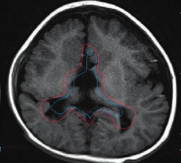
Figure 3: 2D CNN.
3.5. Spatial Convolution Contrast Experiment. The goal of 2D
CNN was providing fine-grained semantic information
about smaller and less salient objects for accurate seg-
mentation. Therefore, the high spatial resolution must be
retained in the output feature map. A simple reduction of the
pooled or stepped convolution layer resulted in a reduction
of the receptive field. Therefore, the cavity convolution was
proposed to enlarge the receptive field and the resolution of
the feature map was maintained. To study whether the hole
convolution helped to learn fine-grained semantic infor-
mation, it was compared with the standard 2D convolution
1 version (HSN-N). The standard 2D convolution version
(HSN-N) had the same architecture as HSN, but all 2D
Figure 4: 3D CNN. convolution layers did not use hole convolution. The con-
volution kernels with large void ratios may be too sparse to
capture local features, which led to the “grid problem.” To
category imbalance. The GDL loss function was used to solve investigate the effect of large void rate on segmentation
the class imbalance problem in CT images. Since many performance, another HSN model (2D HSN-L) with larger
works proved that Dice loss can obtain more reliable results void rate was evaluated. The void rate of the original HSN
than cross-direction loss, there was a performance difference was increased from three to five by this model. Figure 8
between Dice loss and GDL loss. Figures 5 and 6 show the shows the qualitative segmentation results of different ex-
average DSC on the validation set, and the loss of the model periments on the test set. The blue represented the gold
trained with GDL was smaller than the loss of the model standard, and red represented the result of automatic6 Journal of Healthcare Engineering
0.6 0.25
0.5
0.2
0.4
0.15
GDL
Dice
0.3
0.1
0.2
0.05
0.1
0 0
0.26078
5.0141
9.01001
11.67396
14.52072
16.6362
20.24036
22.14691
29.74699
33.37726
38.88797
42.49213
46.8798
54.11424
68.55699
73.70206
77.33234
86.65614
94.62186
GDL
Dice
Figure 5: Training process of different loss function.
1 0.9
0.9 0.8
0.8 0.7
0.7 0.6
0.6
0.5
GDL
Dice
0.5
0.4
0.4
0.3 0.3
0.2 0.2
0.1 0.1
0 0
4.56827
10.07923
16.8374
19.79592
24.23369
29.30957
34.35645
39.02626
42.82592
50.22221
54.02187
57.82153
63.53553
68.81444
73.25222
78.3281
86.9716
96.92033
103.47547
GDL
Dice
Figure 6: The average DSC of the verification set of different loss functions.
1
0.8
0.6
DSC
0.4
0.2
0
Median Mean ± std
HSN
HSN Dice
HSN-3D
Figure 7: Quantitative results of the test set.
segmentation. These segmentation results showed that HSN 3.6. Results of Children’s Rehabilitation Data. The SPECT
performed well in segmenting lung cancer even in a small examination showed hypoperfusion of cerebral blood flow
area. This was because the model can learn remote 3D and decreased functional activity of neurons in the treatment
context information and fine-grained 2D semantic group before treatment, and 27 cases returned to normal
information. after treatment (96.4%). There were 29 cases ofJournal of Healthcare Engineering 7
(a) (b) (c)
Figure 8: Qualitative segmentation results of different experiments on the test set (red was the artificial segmentation area, and blue was the
model segmentation area). (a) HSN; (b) HSN-Dice; (c) HSN-S3D.
70 ∗
hypoperfusion of cerebral blood flow and decreased func-
tional activity of neurons in the control group before 60
treatment, and 6 cases returned to normal after treatment 50
(20.7%). The return to normal rate of SPECT in the treat- 40
DQ
ment group was significantly higher than that in the control 30
group (XPINGFANG � 33 5191, P < 0.001). The cerebral 20
hemodynamic changes of the two groups of children before 10
and after treatment showed that VP of the cerebral artery in
0
children was (139.68 ± 15.66) cm/s after treatment, which HSN technique No HSN technique
was significantly faster than that before treatment
Big action Personal social
(131.84 ± 15.93) cm/s, P < 0.05. The cerebral artery PI of the Fine motor Language
children was 0.91 ± 0.19 after treatment, which was signifi- Social adaptation
cantly lower than that of 1.18 ± 0.24 before treatment,
Figure 9: Changes in DQ of the two groups of children before and
P < 0.05. However, in the control group, the cerebral artery
after treatment (∗ indicated significant difference.).
VP and PI of the children had no significant difference
before and after treatment, P > 0.5. After treatment, there
were significant differences in VP and PI between groups 70 ∗
(P < 0.05). The changes in DQ of the two groups of children 60
before and after treatment are shown in Figure 9. The dif- 50
ference of GM FM scale scores before and after treatment in
40
GMFM
the two groups of children is shown in Figure 10.
30
20
4. Discussion 10
0
A large amount of image data was generated in the process of HSN technique No HSN technique
diagnosis and treatment of CP lesions. These data were
usually subjectively evaluated by doctors based on experi- CMFM I CMFM IV
CMFM II CMFM V
ence, and then the corresponding diagnosis and treatment CMFM III
plan were made. However, the features observed by doctors
with only naked eyes from image data were very limited, and Figure 10: Difference of GM FM scale scores before and after
the potential of image data was often not fully utilized. For treatment in the two groups of children (∗ indicated significant
many years, the quantitative information that was not difference).
available to the human eye was extracted by many scholars
with the help of complex mathematical and statistical al-
gorithms, based on which the corresponding diagnosis and disease. Thus, an important research direction of AI tech-
treatment plan were carried out, and even the progress of the nology in the field of medical applications was constituted
disease was predicted. The image omics came into being with [13–17].
the development of AI technology. The machine learning In recent years, with the rise of deep learning technology
algorithms were used to mine high-throughput features and computer vision technology, it has become more and
from medical images and perform modeling analysis [12]. more urgent to develop automatic segmentation algorithms
More and more evidence showed that imaging omics can be with high accuracy and high stability [9]. The problem of CT
used for the quantitative characterization of CP lesions for image segmentation was studied based on the brain MRI and
the diagnosis, treatment planning, and prognosis of the lung CT images and the use of deep learning technology. In8 Journal of Healthcare Engineering
addition, for the grading of brain lesions, the impact of deep segmentation. After treatment, six patients in the artificial
learning segmentation results and manual segmentation intelligence group returned to normal (20.7%), which was
results on imaging omics research was compared in the significantly higher than the control group (X2 � 335191,
research. For the prediction of chemotherapy outcomes in P < 0.001). Cerebral hemodynamic changes were obvious in
patients with CP, imaging omics models were also con- both groups before and after treatment. VP of the cerebral
structed and analyzed in combination with clinical features. artery was (139.68 ± 15.66) cm/s after treatment, which was
The reproducibility of imaging omics research was still an greatly faster than that before treatment (131.84 ± 15.93) cm/
unresolved problem, and the clinical application of imaging s, P < 0.05. In general, the deep learning model can effec-
omics was greatly affected by this problem. Studies showed tively segment the CP area and assist in the clinical case
that more than 90% of research had not undergone rigorous measurement and diagnosis of future CP children. In ad-
external verification and lacked multicenter diversity data dition, the deep learning model can improve medical effi-
[18, 19]. A hybrid segmentation network based on deep ciency and accurately identify patients’ focal areas, which has
learning (HSN) was used for CT brain image segmentation great application potential in helping to identify the reha-
and the accuracy of image analysis of brain cell function in bilitation training results of children with CP.
children with CP can be improved. The language function,
motor function, cognitive function, language quotient, great Data Availability
motor development quotient, fine motor development
quotient, personal social, and social adaptation development No data were used to support this study.
of the brain of children with CP in the HSN group were
significantly improved after treatment compared to before Conflicts of Interest
treatment.
In this research, a hybrid segmentation network HSN The authors declare that they have no conflicts of interest.
based on deep learning was proposed for CT brain tissue
image segmentation. CT images often have higher resolution
than MRI images. How to segment CT images effectively is
References
always a difficult problem. HSN can effectively solve this [1] M. J. Maenner, S. J. Blumberg, M. D. Kogan, D. Christensen,
problem. HSN includes a lightweight 3D CNN and a refined M. Yeargin-Allsopp, and L. A. Schieve, “Prevalence of cerebral
2D CNN. 3D CNN uses desampled images and spatio- palsy and intellectual disability among children identified in
temporal separable 3D convolution to reduce memory re- two U.S. National Surveys, 2011-2013,” Annals of Epidemi-
quirements and computational costs. 2D CNN can learn ology, vol. 26, no. 3, pp. 222–226, 2016, Epub 2016 Jan 12.
fine-grained semantic information while maintaining a high PMID: 26851824 PMC5144825.
spatial resolution. A hybrid feature fusion module was [2] A. Hosny, C. Parmar, J. Quackenbush, L. H. Schwartz, and
H. J. W. L. Aerts, “Artificial intelligence in radiology,” Nature
proposed to effectively integrate 2D and 3D features. This
Reviews Cancer, vol. 18, no. 8, pp. 500–510, 2018, PMID:
network structure combines the advantages of 3D CNN 29777175 PMC6268174.
learning long-range contextual information and 2D CNN [3] L. Oakden-Rayner, “The rebirth of CAD: how is modern AI
learning semantic information. The results showed that this different from the CAD we know?” Radiology: Artificial In-
model can segment CP lesion area accurately on CT images. telligence, vol. 1, no. 3, Article ID e180089, 2019.
The development of deep learning and imaging omics has [4] W. L. Bi, A. Hosny, M. B. Schabath et al., “Artificial intelli-
promoted the progress of medical imaging. Radiology using gence in cancer imaging: clinical challenges and applications,”
artificial intelligence can automate certain clinical tasks to CA: A Cancer Journal for Clinicians, vol. 69, no. 2, 2019.
some extent. In addition, it can reduce the heavy workload of [5] B. Koçak, E. Ş Durmaz, E. S. Durmaz, E. Ates, and
doctors and improve the diagnostic efficiency, so as to O. Kilickesmez, “Radiomics with artificial intelligence: a
practical guide for beginners,” Diagnostic and interventional
optimize the allocation of social medical resources. How-
radiology, vol. 25, no. 6, pp. 485–495, 2019, PMC6837295.
ever, there are still some shortcomings, which need to be [6] K. Chang, A. L. Beers, H. X. Bai et al., “Automatic assessment
further strengthened in the future. For example, traditional of glioma burden: a deep learning algorithm for fully auto-
image omics feature extraction methods have certain limi- mated volumetric and bidimensional measurement,” Neuro-
tations without adoption of deep learning in feature ex- Oncology, vol. 21, no. 11, pp. 1412–1422, 2019, PMC6827825.
traction. Deep learning methods, especially CNNs, can learn [7] Z. Qian, Y. Li, Y. Wang et al., “Differentiation of glioblastoma
rich texture information from medical images in a hierar- from solitary brain metastases using radiomic machine-
chical manner. Deep features have a more powerful feature learning classifiers,” Cancer Letters, vol. 451, pp. 128–135,
representation than hand-designed features. In the future 2019, Epub 2019 Mar 13. PMID: 30878526.
work, we will carry out related studies on feature extraction [8] Q. Hu, L. F. de F Souza, G. B. Holanda et al., “An effective
based on deep learning to further explore the potential of approach for CT lung segmentation using mask region-based
convolutional neural networks,” Artificial Intelligence in
image data.
Medicine, vol. 103, 2020 Epub 2020 Jan 8. PMID: 32143797,
Article ID 101792.
5. Conclusion [9] S. A. Taghanaki, K. Abhishek, J. P. Cohen, J. Cohen-Adad, and
G. Hamarneh, “Deep semantic segmentation of natural and
In this study, a hybrid segmentation network HSN based on medical images: a review,” Artificial Intelligence Review,
deep learning was proposed for CT brain tissue image vol. 54, no. 1, pp. 137–178, 2020.Journal of Healthcare Engineering 9
[10] X. Zhu, D. Dong, Z. Chen et al., “Radiomic signature as a
diagnostic factor for histologic subtype classification of non-
small cell lung cancer,” European Radiology, vol. 28, no. 7,
pp. 2772–2778, 2018, Epub 2018 Feb 15. PMID: 29450713.
[11] R. Palisano, P. Rosenbaum, S. Walter, D. Russell, E. Wood,
and B. Galuppi, “Development and reliability of a system to
classify gross motor function in children with cerebral palsy,”
Developmental Medicine and Child Neurology, vol. 39, no. 4,
pp. 214–223, 1997.
[12] S. Rizzo, F. Botta, S. Raimondi et al., “Radiomics: the facts and
the challenges of image analysis,” European Radiology Ex-
perimental, vol. 2, no. 1, p. 36, 2018 PMID: 30426318
PMC6234198.
[13] T. Kagawa, S. Yoshida, T. Shiraishi et al., “Basic principles of
magnetic resonance imaging for beginner oral and maxillo-
facial radiologists,” Oral Radiology, vol. 33, no. 2, pp. 92–100,
2017.
[14] P. Korfiatis, T. L. Kline, Z. Akkus et al., Predictive Modeling,
Machine Learning, and Statistical Issues, CRC Press, Boca
Raton, Florida, 2019.
[15] M. Shafiq-Ul-Hassan, G. G. Zhang, K. Latifi et al., “Intrinsic
dependencies of CT radiomic features on voxel size and
number of gray levels,” Medical Physics, vol. 44, no. 3,
pp. 1050–1062, 2017, PMID: 28112418 PMC5462462.
[16] C. A. Owens, C. B. Peterson, C. Tang et al., “Lung tumor
segmentation methods: impact on the uncertainty of radio-
mics features for non-small cell lung cancer,” PLoS One,
vol. 13, no. 10, PMID: 30286184 PMC6171919, Article ID
e0205003, 2018.
[17] H. Seo, M. Badiei Khuzani, V. Vasudevan et al., “Machine
learning techniques for biomedical image segmentation: an
overview of technical aspects and introduction to state-of-art
applications,” Medical Physics, vol. 47, no. 5, pp. e148–e167,
2020 Jun, PMID: 32418337 PMC7338207.
[18] G. Wang, W. Li, S. Ourselin, and T. Vercauteren, “Automatic
brain tumor segmentation using cascaded anisotropic con-
volutional neural networks,” International MICCAI Brainle-
sion Workshop, Springer, New York, NW, USA, 2017.
[19] Y. Yuan, M. Chao, and Y.-C. Lo, “Automatic skin lesion
segmentation using deep fully convolutional networks with
jaccard distance,” IEEE Transactions on Medical Imaging,
vol. 36, no. 9, pp. 1876–1886, 2017, Epub 2017 Apr 18. PMID:
28436853.You can also read