University of Nebraska UAS profiling during LAPSE-RATE
←
→
Page content transcription
If your browser does not render page correctly, please read the page content below
University of Nebraska UAS profiling during LAPSE-RATE
     Ashraful Islam1 , Ajay Shankar1 , Adam Houston2 , and Carrick Detweiler1
     1
         NIMBUS Lab, Department of Computer Science & Engineering, University of Nebraska-Lincoln, Lincoln, NE 68588, USA.
     2
         Department of Earth & Atmospheric Sciences, University of Nebraska-Lincoln, Lincoln, NE 68588, USA.
     Correspondence: Ashraful Islam (mislam@huskers.unl.edu)

     Abstract.
          This paper describes the data collected by the University of Nebraska-Lincoln (UNL) as part of the field deployments during
     the Lower Atmospheric Process Studies at Elevation — a Remotely-piloted Aircraft Team Experiment (LAPSE-RATE) flight
     campaign in July 2018. UNL deployed two multirotor unmanned aerial systems (UASs) at multiple sites in the San Luis Valley
5    (Colorado, USA) for data collection to support three science missions: convection-initiation, boundary layer transition, and cold
     air drainage flow. We conducted 172 flights resulting in over 21 hours of cumulative flight time. Our novel design for the sensor
     housing onboard the UAS was employed in these flights to meet the aspiration and shielding requirements of the temperature
     and humidity sensors and to separate them from the mixed turbulent airflow from the propellers. Data presented in this paper
     include timestamped temperature and humidity data collected from the sensors, along with the three-dimensional position and
10   velocity of the UAS. Data are quality controlled and time-synchronized using a zero-order-hold interpolation without additional
     post-processing. The full dataset is also made available for download at (https://doi.org/10.5281/zenodo.4306086 (Islam et al.,
     2020)).

     1     Introduction

     A team of researchers from the University of Nebraska-Lincoln (UNL) participated in the Lower Atmospheric Process Studies
15   at Elevation —- a Remotely piloted Aircraft Team Experiment (LAPSE-RATE) flight campaign between 14 – 19 July 2018 at
     San Luis Valley of Colorado, USA. LAPSE-RATE was organized as part of the International Society for Atmospheric Research
     using Remotely piloted Aircraft (ISARRA) 2018 meeting. A total of 1287 flights were conducted by 13 institutions, including
     UNL, which resulted in more than 260 hours of data collection. UNL’s contribution to this collaborative data collection effort
     was 172 Atmospheric Boundary Layer (ABL) profiling flights using two multirotor UAS platforms. These flights from UNL
20   resulted in over 21 hours of data being collected. This unique collaboration resulted in a collective sampling of a variety of
     atmospheric phenomena over the span of six days at preplanned sites around the San Luis Valley. An overview of the LAPSE-
     RATE campaign, the description of site locations, and science missions that focused on measuring different atmospheric
     phenomena of interest are documented (de Boer et al., 2020a, b). Data from UNL and all other participating teams in the
     LAPSE-RATE campaign are hosted in an open access data repository (LAPSE-RATE Data Repository, 2021).
25        Multirotor UASs are finding more routine uses for sampling and profiling the ABL, such as atmospheric profiling (Bonin
     et al., 2013; Elston et al., 2015; Greatwood et al., 2017; Jacob et al., 2018; Islam et al., 2019; Barbieri et al., 2019; Segales

                                                                     1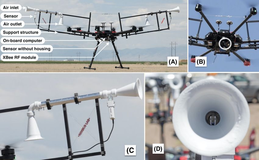
et al., 2020), estimation of the spatial structure of temperature (Hemingway et al., 2020), wind measurement (Prudden et al.,
     2016; Palomaki et al., 2017), and prediction of Lagrangian coherent structure (Nolan et al., 2018).
       The need for increased spatial resolution for atmospheric sampling is reflected in publications, such as improving Numerical
30   Weather Prediction (NWP) models (Leuenberger et al., 2020), improvement of mesoscale atmospheric forecast (Dabberdt
     et al., 2005), and identification of hazardous weather for Beyond Visual Line of Sight(BVLOS) flights using UAS Traffic
     Management (UTM) systems (Mitchell et al., 2020). UASs can meet such profiling needs with a greater frequency of profiles,
     increased spatiotemporal resolution of data, and sampling in virtually any sampling location when compared with traditional
     methods. Multirotors extend the sampling capability by allowing rapid and repeatable profiling at any site while maintaining a
35   fixed horizontal position.
       Our previous work (Islam et al., 2019) describes the design and evaluation of a temperature and humidity (TH) sensor
     housing that meets the recommended sensor placement, aspiration, and shielding criteria by using a passively induced-airflow
     technique that works by exploiting the existing UAS propeller. The housing’s inlet is pointed outwards from the UAS to
     sample just outside of the UAS turbulence in both ascent and descent. This is different from existing methods of placing the
40   sensor under the arm without shielding but aspirated by the propeller (Hemingway et al., 2017), on the body of the UAS
     without shielding and aspiration (Lee et al., 2018), on a different part of the UAS with shielding and possible aspiration from
     propellers (Greene et al., 2018) or shielding the sensor inside UAS and active aspiration using a fan while pointing the inlet
     towards the wind (Greene et al., 2019). All of these existing configurations fail to produce reliable data during descent, and
     these data are usually discarded (Lee et al., 2018). As multirotor flight time is very limited, needing to discard entire descent
45   data prevents optimal use of resources. Additionally, in most cases, observations are affected by wind direction and require
     onboard sensing of wind and reorientation of UAS with the change of wind direction (Greene et al., 2019).
       Two primary highlights of our novel sensor housing are its ability to obtain temperature and humidity sensor readings
     reliably during both ascent and descent profiles, and its invariance to the aircraft orientation relative to the ambient wind. Two
     key design considerations in achieving these goals are: the placement of the sensor, and its consistent aspiration. Placement
50   of the sensor on the UAS body can adversely affect the measurements (Greene et al., 2018; Jacob et al., 2018). As observed
     through prior experimental results (Villa et al., 2016), the accuracy of a sensor’s measurement increases the farther away it is
     placed from the propeller’s downwash. More specifically, a sensor placed at a distance at least 2.5 times the propeller diameter
     away from the rotor experiences significantly less aerodynamic interference (Prudden et al., 2016). Consistent and sufficient
     aspiration is also necessary for a consistent effective sensor response time (Houston and Keeler, 2018). Placing the sensor
55   inside the propeller region or near the body can result in inconsistent aspiration due to rotor turbulence (Diaz and Yoon, 2018;
     Yoon et al., 2017). As such, we designed our sensor housing to source the sampling air from outside rotor interference and to
     maintain consistently high aspiration airspeed to obtain reliable results.
       Our sensor housing design has evolved over multiple design iterations and has been field-tested in multiple Collaboration
     Leading Operational UAS Development for Meteorology and Atmospheric Physics (CLOUD-MAP) field campaigns (Jacob
60   et al., 2018). The details of our data validations tests, as well as a complete description of the sensor housing design, are
     available in a separate open access paper (Islam et al., 2019).

                                                                       2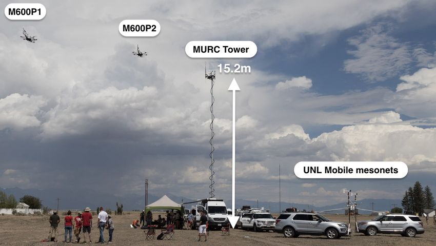
Figure 1. Images of (A) the UAS setup with the temperature and humidity sensor mounted in the aspirated and shielded sensor housing, and
     in a traditional configuration (B) Close up of the traditionally mounted sensor under the UAS without the sensor housing (inside the white
     circle), (C) Close up of the sensor housing with the sensor mounted, and (D) Close up of the sensor probe mounted inside our sensor housing.
     The outlet of the sensor housing is placed on top of the propeller, and the inlet is pointing outward. High-speed air in the sensor housing is
     drawn passively by exploiting the pressure deficit created by the propeller of the UAS.

       For the LAPSE-RATE campaign, UNL deployed two identical UASs with one primary sensor suite for measurements, and a
     secondary sensor suite for redundancy and testing. These flights were conducted at five locations in San Luis Valley (Colorado,
     USA) through 14–19 July 2018. The maximum altitude for each flight ranged from 100 − 500 m above ground level. Figure 1
65   illustrates the UAS with the housing setup, closeup of the sensor housing, and sensor mounting configurations. Both primary
     and secondary sensors are located inside their respective sensor housings mounted on two diametrically opposing arms of the
     UAS. In some flights, a third sensor was mounted under the body frame of the UAS to compare the performance of primary
     sensors against traditional mounting positions. A detailed description of our configuration is presented in Section 2.5. It should
     be noted that, although the data collection is focused on the temperature and humidity measurements, atmospheric pressure
70   data from the sensors are also included in the dataset for anyone interested.

                                                                           3
The rest of the paper describes the components of our system (Section 2), the flight strategies employed for missions (Section
3), the data processing used (Section 4), and some special topics of interest (Section 5). We finally conclude with an example
profile data, and provide details regarding the availability of the dataset.
2 System Description
75 2.1 UAS platform
The two identical UASs deployed during the missions were developed on a DJI Matrice 600Pro platform equipped with DJI
A3 Pro flight control systems. The unfolded dimensions (including propellers, frame arms, GPS mounts, and landing gear) of
the system are 1668 mm × 1518 mm × 727 mm. The recommended maximum payload capacity of the platform is 5.5 kg. At
no load, the UAS has a flight endurance of 35 − 40 min on a single set of six DJI TB48S batteries. The manufacturer-specified
80 positioning accuracy is ± 0.5 m in the vertical axis, and ± 1.5 m horizontal (DJI, 2021b). The maximum ascent and descent
speeds are 5 m s−1 and 3 m s−1 , respectively. The flight controller offers real-time access (read-only) to UAS’s onboard sensor
data, such as position, velocity, and attitude, through a serial interface. Additionally, a mobile application allows a user to plan
and deploy a flight trajectory, and the remote controller allows intervention from the user at any point.
2.2 Sensors
85 Table 1 describes the specifications of the temperature and humidity (TH) sensors used for the dataset. Every UAS flight used
one iMet XQ2 from InterMet Systems (Grand Rapids, MI, USA) as the primary TH sensor. The XQ2 is a self-contained sensor
package designed for UASs to measure atmospheric pressure, temperature, and relative humidity. It is also equipped with a
built-in GPS and an internal data logger along with a rechargeable battery. A serial interface provides access to the logs, or
real-time observations produced by the sensor at 1 Hz. The internal data-logger was only used as backup and is not part of this
90 dataset. Data included in the dataset were collected through the data acquisition (DAQ) system using the serial interface. Some
UAS flights featured an older version of this sensor, called iMet XQ1, as the secondary backup sensor.
Some flights also used a nimbus-pth as the secondary sensor, which is a sensor package unit we designed and built for
pressure, temperature, and humidity sensors. Several nimbus-pth can be chained as nodes for data collection. In some data
files, two of these nodes might be present. In such cases, one of them was aspirated inside our sensor housing, and the other
95 one sat directly underneath the UAS in a traditional non-aspirated configuration. In the data files, the first two sensors were
shielded and aspirated inside the housing, and the third sensor (when available) was in a traditional non-aspirated configuration.
2.3 Sensor Housing
The sensor housing is designed to meet or exceed sensor placement requirements, such as consistent aspiration for the sensors,
shielding from solar radiation and other indirect heat sources. The housing draws air passively by exploiting the pressure
100 differential between the region just above a propeller and the region just beyond the rotor wash. The airflow through the
4Table 1. The key manufacturer’s specifications for the sensors used in different experiments: The unavailable fields are left blank. Datasheet
for each sensor packages are available at iMet XQ2 (InterMet Systems, 2021b), iMet XQ1 (InterMet Systems, 2021a), and nimbus-
pth (Digikey, 2021; Mouser, 2021)
XQ2 XQ1 nimbus-pth
(iMet XQ2) (iMet XQ1) (Custom Built)
Type Bead Thermistor Bead Thermistor Bead Thermistor
Temperature
◦ ◦
Range −90 to 50 C −95 to 50 C −40 to 100 ◦ C
Response Time 1 s @ 5 m s−1 2s
◦
Resolution 0.01 C 0.01 ◦ C 0.01 ◦ C
Accuracy ± 0.3 ◦ C ± 0.3 ◦ C
Type Capacitive Capacitive Capacitive
Range 0 − 100 % RH 0 − 100 % RH 0 − 100 % RH
◦ −1
Humidity
@ 25 C, 0.6 s 5s @ 1ms velocity 8s
◦
Response Time @ 5 C, 5.2 s
@ −10 ◦ C, 10.9 s
Resolution 0.1 % RH 0.7 % RH 0.01 % RH
Accuracy ± 5 % RH ± 5 % RH ± 2 % RH
housing is always maintained as long as the propellers are spinning, and provides a consistent aspiration for the sensors (Islam
et al., 2019). The inlet and outlet of the housing are shaped like a cone to provide high-speed airflow across the housing tube
with a small pressure difference between the two ends. Additional design considerations are made to ensure that the flow is
consistent, and provides airflow ≥ 5 m s−1 across the sensors even at the lowest propeller speeds.
105 Sensors are placed inside the tube structure as shown in the panel C and D of Figure 1. The entire sensor housing is painted
with reflective white paint, and tubes are wrapped with aluminum foil tape. This results in excellent rejection of solar heating
and avoids unpredictable radiation heating bias. Such placement of sensors provides solar shielding and shielding from other
artificial heat sources such as motor or battery waste heat. Since the entire housing is placed outside the body of UAS, it creates
further isolation from the artificial heat sources in the UAS. Additionally, since the aspirating airspeed is very high (Islam et al.,
110 2019), it reduces the error from all these sources even further (Anderson and Baumgartner, 1998).
The housing is also designed to be modular, printed entirely using a 3D printer, and has an easy screw-in assembly. The
impact of the housing on the UAS’s stability and flight time is minimal. Further details and the full schematic of the housing
and the evaluation can be found in our previous work (Islam et al., 2019).
2.4 Data acquisition
115 Data were collected using a data acquisition (DAQ) system comprised of an Odroid XU4 (Hardkernel, 2021), a compact
single-board computer that runs a Linux operating system. Odroid runs the robot operating system (ROS) (Quigley et al.,
52009) that communicates with the serial devices through its USB ports. ROS facilitates collecting many different sensor data
independently at their own output frequency, recording the timestamp for when data were generated and when they are received
by ROS. ROS interfaces the collection of all available devices even in the case of a single device failure. Synchronization of
120 the data can either be done at runtime or in post-processing. In our case, it was done in post-processing using MATLAB.
The communication with the DJI flight controller was implemented using the ROS interface of DJI Onboard SDK (DJI,
2021c) available to developers. This allowed the recording of all the telemetry data from the flight controller, along with
high-quality positioning information. The GPS data from the iMet XQ2/ iMet XQ1 sensor were discarded as the positioning
information from the flight controller was found to be of better quality.
125 The Odroid was connected with a ground computer using wireless 2.4 GHz XBee radios for the operation of DAQ, debug-
ging, and periodic checks on the data when the UAS finished a flight. The data collected by the DAQ were retrieved to the
ground computer for archiving at the end of each day using an ethernet connection.
Temperature and humidity sensors were connected over serial with ROS to send periodic updates of the observations. The
UAS’s autopilot also interfaced with ROS to provide updates of position, velocity, altitude, attitude, etc. which were also
130 recorded to spatially and temporally synchronize the observation.
2.5 UAS Sensor Mounting Configuration and Payload
As mentioned in Subsection 2.2, the primary sensor was the iMet XQ2, and its data were recorded on the dataset with a header
underscore _1 (e.g., Temperature_1, Humidity_1, Pressure_1). Other sensor data headers were followed with _2 and _3 when
available. Sensor_1 and Sensor_2 were shielded inside the sensor housing; however, sensor_3 was placed under the UAS in a
135 traditional configuration without aspiration. The placement of the sensors inside the housing and sensors without the housing
are marked in Figure 1 for reference. Specific placements of the sensors on the UAS used in the data collection are described
below.
2.5.1 UAS platform M600P1
One XQ2 (sensor_1) was placed inside the left sensor housing, and one XQ1 (sensor_2) was on an identical right sensor
140 housing. This placement location for the left housing is highlighted in the ‘panel (A)’ of Figure 1. The alternative setup used
in some experiments replaced XQ1 with nimbus-pth (sensor_2) inside the right sensor housing (sensor names are also listed
in metadata as data source). If nimbus-pth is included in measurements, it was placed under the body of the UAS without any
housing structure, as highlighted in the ‘panel (A)’ and ‘panel (B)’ of Figure 1.
2.5.2 UAS platform M600P2
145 One XQ2 (sensor_1) was mounted inside the left sensor housing, one nimbus-pth (sensor_2) was mounted inside the right
sensor housing, and an additional nimbus-pth (sensor_3) was placed under the body of the UAS without a housing. This form
of sensor placement facilitates an evaluation between the sensor placed inside the housing versus under the body of the UAS
6Table 2. Latitude, longitude, and mean sea level (MSL) altitude of operation locations in World Geodetic System 84 (WGS 84) decimal
degrees.
Location Latitude Longitude Altitude (MSL)
Golf 37.626963 -105.820028 2298 m
Gamma 37.893536 -105.716137 2329 m
Leach Airfield 37.784560 -106.044552 2316 m
India 38.051294 -106.102885 2332 m
Charlie 38.052690 -106.087414 2329 m
without housing. It also allows comparison of the sensors mounted on the opposite ends of the UAS. Having secondary sensors
also provides a fail-safe when the primary sensors fail, such as the case on XQ2 humidity sensors on 17 July 2018 data.
150 The UAS’s total payload during the experiments was approximately 1.8 kg. Two sensor housings with their support structure
and sensor were approximately 720 g each; the onboard computer was 140 g; and misc cables, screws, etc., were approximately
200 g. UAS flight endurance was 20 − −25 min with the payload.
3 Flight locations and strategies
3.1 Flight locations
155 During the LAPSE-RATE field campaign, measurement objectives for each day were determined based on the weather fore-
cast, site availability, and available team resources. Many designated locations of San Luis Valley of Colorado, USA, were
planned beforehand as atmospheric sampling sites depending on atmospheric phenomena of interest. The planning of loca-
tions, atmospheric phenomenon to be observed for the day, and assignment of teams are described in (de Boer et al., 2020a).
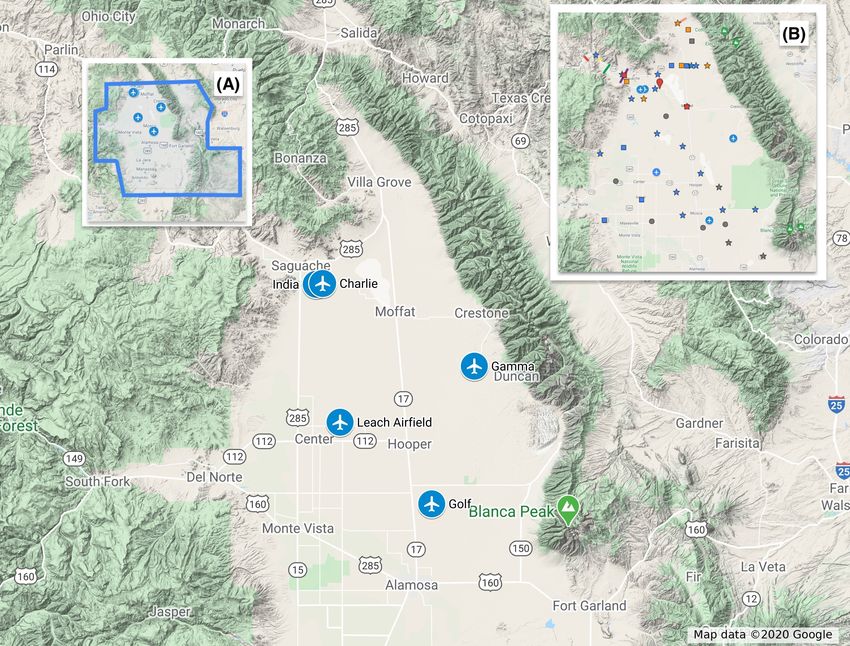
We conducted flights in locations designated as Golf, Gamma, Leach, India, and Charlie between 14 – 19 July as part of the
160 LAPSE-RATE flight campaign (de Boer et al., 2020b) as well as individual research objectives. GPS coordinates of these loca-
tions are provided in Table 2 and illustrated in a terrain map in Figure 2. The ‘inset (B)’ of Figure 2 shows the flight locations
of UNL UASs in the context of all the LAPSE-RATE flight campaign locations of interest where all the teams were operating
based on the measurement objective of the day.
3.2 Flight strategies
165 Flight strategies for each day were dictated by atmospheric phenomena being measured. The teams participating in the LAPSE-
RATE campaign coordinated flights across the San Luis Valley according to the atmospheric phenomena of interest for the day
and the atmospheric variability expected at different sampling locations. Measurement objectives of LAPSE-RATE in which
UNL participated in data collection are calibration flight (CLF), boundary layer transition (BLT), convection initiation (CI),
7Figure 2. Flight locations of UNL UASs overlaid on the terrain map. Inset (A) shows the blue overlay area where operation of small UASs
for flight altitudes up to 914.4 m AGL was authorized by the Federal Aviation Authority (FAA) Certificate of Authorization (COA) between
13 – 22 July. Inset (B) shows the spatial distribution of flight locations used by UNL and all other teams participating in the LAPSE-RATE
campaign for various missions between 14 – 19 July 2018. Map data © Google 2020
8Table 3. UAS locations and mission objectives for the day. Mission objectives are: Calibration flight (CLF), Boundary layer transition (BLT),
Convection initiation (CI), Cold air drainage flow (CDF)
Location
Date and Time Objective No. of Maximum Golf Gamma Leach India Charlie
Flights Altitude
14 July 2018 CLF 2 120 m M600P1 & M600P2
(17:17-17:33 MDT)
15 July 2018 CI 19 500 m M600P1 M600P2
(9:00-15:15 MDT)
16 July 2018 CI 47 120 m M600P1 M600P2
(8:00-14:30 MDT)
17 July 2019 BLT 18 100 m M600P1 & M600P2
(7:00-9:00 MDT)
18 July 2019 CI 43 120 m M600P1 M600P2
(7:00-14:30 MDT)
19 July 2019 CDF 43 500 m M600P1 M600P2
(5:30-11:00 MDT)
cold air drainage flow (CDF). Table 3 shows the locations of UASs deployed by UNL by date, time, and the corresponding
170 mission objectives.
All the flights were conducted under the command of one remote pilot in command (PIC) with ‘Federal Aviation Admin-
istration (FAA) part 107’ license in accordance with FAA’s rule. All the flights included in the dataset were conducted using
preprogrammed missions in DJI Ground Station (GS) Pro app (DJI, 2021a) by the remote pilot in command (PIC), with very
few exceptions of manual flights. Occasionally the remote PIC took control over segments of flight from the automatic mis-
175 sion control of the app when deemed safer by the PIC, e.g., passing through a turbulent layer of atmosphere. Although visual
observers (VO) were not required by FAA, two VO were present at each flight location for greater situational awareness and
safety during each flight. VOs were monitoring the UAS’s movement, took handwritten notes about flight events and weather,
and scanned the surrounding area for manned and unmanned flights.
All the flights were legally conducted under FAA Certificate of Authorization (COA) for altitudes up to 914.4 m AGL when
180 notices to airmen (NOTAMs) were active in the blue area marked in the ‘inset (A)’ of Figure 2. For all our flights, however, we
were limited to flying up to a 500 m maximum altitude due to the altitude limitation set in the firmware of the UAS. In the days
when NOTAMs were not active for COA, all the flights were conducted up to the legal flight limit of 121 m AGL as defined in
the ‘part 107’ regulations.
9Figure 3. Coordinated data collection of the UNL UAS platforms and UNL Mobile Mesonets next to the MURC tower. UAS platforms were
hovering at 15.2 m AGL (the same altitude as MURC tower instrumentation).
3.2.1 14 July 2018
185 On 14 July 2018, the mission objective was to compare both of the systems against a reference point, the Mobile UAS Re-
search Collaboratory (MURC) tower (de Boer et al., 2020c), to calibrate and validate the sensor observations. MURC tower
instrumentations were set to 15.2 m AGL. University of Nebraska-Lincoln (UNL) Mobile Mesonet was also collecting data
about 2 m AGL for surface-level observations. Additionally, periodic radiosonde launches were conducted by National Se-
vere Storms Laboratory (NSSL). Figure 3 shows an overview of the spatial distribution of the MURC tower, UAS platforms,
190 and UNL Mobile Mesonet. Details about MURC tower’s instrumentation, deployment strategies, and data processing can be
obtained from (de Boer et al., 2020c).
One flight for each system was conducted where the UAS ascended to the height of the MURC tower (15.2 m) and hovered
for 10 minutes. After that, the UAS ascended to 120 m at 1 m s−1 , hovered for 30 s, and descended at the same speed to
land. This mission was performed in collaboration with all participating teams at the LAPSE-RATE campaign to provide
195 measurement intercomparison between platforms from all teams (Barbieri et al., 2019). The data are available for the MURC
tower (de Boer et al., 2020c), UNL Mobile Mesonet (de Boer et al., 2020c), radiosonde (Bell et al., 2021), and all other
10participating teams on 14 – 15 July 2018 in the Zenodo community for LAPSE-RATE at (LAPSE-RATE Data Repository,
2021).
3.2.2 15 July 2018
200 On 15 July 2018, the mission objective of the day was convection initiation (CI). Vertical profiling flights were conducted up
to 500 m altitude at 1 m s−1 ascent/descent speed at the Golf and Gamma locations. Flights were planned to be at every 30
minutes to allow recharge of the UAS batteries while cycling through multiple sets of batteries.
At the Golf location, ten flights were conducted between 8:59 – 15:14 MDT (local time). The weather was slightly cloudy
in the morning and clear throughout the rest of the day. Very windy conditions existed for the last few flights.
205 At the Gamma location, nine flights were conducted between 9:02 – 3:15 MDT (local time). Two out of the nine data files
could not be recovered due to an error in the onboard logging computer and a sensor issue. The weather was clear and windy
in the morning, and slightly cloudy for the last half of the flights.
3.2.3 16 July 2018
On 16 July 2018, the scheduled mission objective was also CI with flights at the same locations as the previous day. Flights
210 were limited to 120 m altitude at 1.5 m s−1 ascent/descent speed due to Notice to Airmen (NOTAM) not being active for the
day. Due to reduced altitude, more flights could be conducted with available batteries. As such, flights were conducted every
15 minutes.
We performed 26 flights at Golf between 8:06 – 14:34 MDT (local time). The first two flights of the morning consisted
of two consecutive profiles, but it was draining the battery a lot faster than our recharging capacity. We then switched to one
215 profile every 15 minutes to reserve enough battery in each flight to maintain a consistent interval between profiles. The weather
started slightly cloudy, and then remained clear throughout the day.
At Gamma, 21 flights were conducted between 9:02 – 14:05 MDT (local time). All the profiles collected at this location are
single profiles. The weather was clear throughout the day, with partly cloudy conditions persisting during the last few flights.
3.2.4 17 July 2018
220 On 17 July 2018, the scheduled missions were for boundary layer transition (BLT). The experiments were geared towards
validation of the sensor housing by the detection of the inversion layer. We conducted the experiments in the early morning in
an inversion, before sunrise, to identify if the sensor housing introduces measurement error due to the upwash or downwash of
the UAS. This effect is more easily detected in stable versus well-mixed conditions since air molecules from stable air airmass
will maintain the temperature of the layer even when air is pushed up or down. Thus if we can verify that sensor housing detects
225 inversion at the same level as a standard measurement (such as radiosonde), we know the readings are not affected by upwash
or downwash.
11We conducted simultaneous flights for both UAS with six vertical profiles and three horizontal profiles at various UAS
movement speeds between 7:00 – 8:48 MDT (local time). NSSL launched coordinated radiosonde balloons at regular intervals
at the same location to be used as the ground truth measurement for UAS’s data. UNL Mobile Mesonets collected measurements
230 at 2 m AGL for surface-level observations during the entire duration of the experiments. The sky remained cloudy throughout
all the flights.
3.2.5 18 July 2018
On 18 July 2018, the scheduled mission was for CI. Flights were conducted up to 500 m altitude at 1.5 m s−1 ascent/descent
speed at both Golf and Gamma locations. Flights were generally conducted every 30 minutes.
235 At the Golf location, a total 27 of flights were performed between 7:08 – 14:20 MDT (local time). The first 17 flights
were in support of the LAPSE-RATE campaign objective. At the conclusion of the day, ten additional 150 m altitude flights
were performed at various ascent/descent speeds to study the effect of UAS movement speed on temperature and humidity
observations.
At the Gamma location, 16 profile flights were conducted between 7:07 – 13:12 MDT (local time). At both locations, some
240 flights were performed up to an altitude of 300 m, while others at 500 m.
At both locations, the sky was clear for the first half of the flights, and partly cloudy for the second half.
3.2.6 19 July 2018
On 19 July 2018, the mission objective was cold drainage flow. UASs were placed at the Charlie and India locations for this
mission. Flights were performed starting before sunrise at 1.5 m s−1 ascent/descent speed. Flights were scheduled for every 15
245 minutes. Strobe lights, as per FAA regulations, were used for flights during twilight.
At the India location, 23 flights were conducted between 5:34 – 11:08 MDT (local time). Maximum flight altitudes were up
to 300 m AGL for seven flights, 350 m AGL for 15 flights, 500 m AGL for one flight.
At the Charlie location, 21 flights were performed between 5:50 – 11:10 MDT (local time). Maximum flight altitudes were
up to 300 m AGL for ten flights, 350 m AGL for nine flights, 500 m AGL for one flight.
250 At both locations, the sky was cloudy before sunrise but clear afterward.
4 Data processing and quality control
Data are recorded from individual sensors and the UAS flight controller as they arrive at the DAQ, as described earlier. The
recorded data are then processed in MATLAB to synchronize using the zero-order-hold (ZOH) method to create a single output
file. We used a discrete sample time of 1 s for zero-order-hold to match the output rate of primary sensors. In the ZOH method,
255 sample value is held constant for one sampling period, i.e., when temperature data is recorded from temperature sensors, the
last known value of altitude from GPS data is recorded without any interpolation. Since the GPS data is recorded at a higher
frequency from the flight controller, it is assumed to be close and within GPS’s uncertainty of measurement. Invalid or missing
12data are replaced with -9999.9 wherever the sensor data are unavailable to the DAQ. No other processing was done on the data,
such as sensor response correction, bias correction, etc.
260 We note that the humidity observations of the primary sensor on some flights for 17 July 2018 were saturated at 100% in one
of the UAS (M600P1), and the corresponding data are not usable. Secondary sensor measurements should be used to replace
these data. Also, humidity readings from nimbus-pth have sensitivity issues; although it displays a similar trend as the other
sensors, it does not capture the whole range of observation and will need further calibration.
Files were formatted in NetCDF format, with common variables names and meta-data added, to be consistent with all the
265 entities collecting data for the LAPSE-RATE field campaign. A detailed explanation of the naming conventions and meta-data
that were requested can be obtained from (de Boer et al., 2020b). An example file name produced by UAS platforms M600P1,
and M600P2 for the data collected starting at 23:16:33 UTC on 14 July 2018 would be UNL.MR6P1.a0.20180714.231633.nc,
and UNL.MR6P2.a0.20180714.231633.nc respectively. Here,
– ‘UNL’ is the identifier for the data collecting institution, UNL
270 – ‘MR6P1’, and ‘MR6P2’ are the platform identifiers for M600P1, and M600P2 respectively
– ‘a0’ indicates raw data converted to NetCDF
– ‘20180714’ is UTC file date in yyyymmdd(year, month, day) format
– ‘231633’ is UTC file start time in hhmmss(hours, minutes, seconds) format
– ‘nc’ is the NetCDF file extension
275 All the files also contain metadata for each variable with an explanation of physical measurement units, time synchronization
method, sensors used for the measurement. File naming conventions and explanations are also described in the read-me file of
the Zenodo data repository.
5 Special topics of interest
The following are special topics of interest that can be studied from the dataset. Our analysis that focused on these topics can
280 be found in our previous work (Islam et al., 2019).
5.1 Calibration
Data from 14 July 2018 can be used with MURC data available at the Zenodo data repository (de Boer et al., 2020c) to obtain
a for calibration. Correction of bias in sensor readings during post-processing requires calibration against a known reliable
measurement. It also serves as additional validation for the sensor platforms and their collected data. It also facilitates the com-
285 parison of data collected by different platforms by providing a “ground-truth” to compare against. Our previous paper (Islam
et al., 2019) discusses the deviation of our observations with MURC data over a period of 10 minutes. Other work (Barbieri
13et al., 2019) compares all the different platforms participating in the LAPSE-RATE campaign along with ours against MURC
tower data.
5.2 Effect of ascent/descent speed
290 Ten flights from the M600P1 platform on 18 July 2020 starting at 20:21 UTC (local time 14:21 MDT) can be used to study the
effect of ascent/descent speed on the sensor readings. Flights were conducted up to a 150 m altitude with speeds ranging from
1 − 5 m s−1 ascent speed, and 1 − 3 m s−1 descent speed. While it is desirable to move at a faster speed to optimize battery
power usage to profile at greater altitudes, it may contribute to the effective sensor response time. Characterizing the sensor
response at the different ascent and descent speeds would allow for the corresponding correction in the post-processing of the
295 data. Our analysis of these data can also be found in our paper (Islam et al., 2019).
5.3 Detection of Inversion
The first six flights from each platform can be used from 17 July 2020 to study the sensor performance within an inversion layer.
The speed of flight through the inversion layer ranged from 0.5 − 5 m s−1 for ascent, and 0.5 − 3 m s−1 for descent. The flights
were coordinated with radiosonde launches from National Severe Storms Laboratory (NSSL) to compare the UAS profiles
300 against the radiosonde profiles. University of Nebraska-Lincoln (UNL) Mobile Mesonet was also collecting data at the ground
for surface-level observations. Dataset for radiosonde observations by NSSL (Bell et al., 2021), and surface observations by
UNL Mobile Mesonet (de Boer et al., 2020c) is uploaded to Zenodo for intercomparison. The ability to detect the inversion at
the correct altitude by the UAS sensor proves that UAS is collecting the observations at the sensor level rather than from the
upwash or downwash of the UAS. Additionally, detection of inversion provides confidence in the quality of the data from the
305 sensor housing in both ascent and descent. Different ascent descent speeds are used to identify the maximum speed that can be
used while still acquiring quality data. Characterization of the sensor in the inversion layer provides a means for correction of
observation level in case an offset is detected in the inversion layer when compared to a radiosonde. These data could also be
used for comparison to the theoretical work for ascent and descent rate of sensing platforms (Houston and Keeler, 2020).
5.4 Effect of body-relative wind direction and Horizontal transect
310 Data are available to study sensor performance during horizontal transect with different orientations relative to the wind.
The last three flights from each platform on 17 July 2020 can be used for this purpose. Horizontal flight speed ranged from
2 − 10 m s−1 . These data can also be compared with radiosonde profile (Bell et al., 2021) and surface observations (de Boer
et al., 2020c) similar to Section 5.3. The horizontal flights at different speeds against various orientations of wind provide
additional characterizations for the quality of sensor data at various atmospheric wind conditions. Different horizontal flight
315 speed simulates different incident wind speed at the sensor housing inlet and their effect on the observations. At the same time,
the orientation of sensor housing simulates incident wind at different orientations and their effects on the sensor observations.
The orientation characterization is particularly important as waste heat from UAS can be carried into the sensor housing in
14an unfavorable wind orientation. Any bias that may appear in these tests would need to be considered in the profiling flight
plan to optimize the orientation of the sensor housing inlet relative to the wind to collect quality data and make appropriate
320 corrections in the post-processing. Our analysis of these data can also be found in our previous work (Islam et al., 2019).
Although traditionally multirotor UAS is used for vertical profiling; our data shows reliable data collection is also possible for
horizontal profile/transect using our sensor housing.
6 Examples of collected profile
Figure 4 shows examples of temperature and humidity profiles collected using the M600P1 platform’s primary sensor. The top
325 two panels illustrate a 500m profile taken through a well-mixed atmosphere. The bottom two panels in Figure 4 are an example
of a profile taken before sunrise through a nocturnal inversion. Although the housing is designed to address ascent/descent
differences, the sensor and the housing have an inherent response time that can not be eliminated. The utility of the presented
sensor housing is to keep the effective response time consistent irrespective of the atmospheric condition or orientation of the
sensor relative to the wind/sun. The data presented in the figures are not filtered or corrected for effective sensor response
330 time. The raw data without any sensor response correction is presented to show the impact of proper sensor housing on the
observations collected by temperature and humidity sensors. This response lag causes a deviation in ascent/descent reading
as is expected. Ascent/descent deviation for humidity sensor is larger due to its slower response time in colder temperatures.
Even without any correction, ascent and descent readings in our data were within the bounds of sensors uncertainty (± 0.3 ◦ C
and ± 5 % RH for temperature and humidity sensors, respectively) and show how effective sensor housing is in collecting
335 quality data. It should be noted that correction can be done using sensor response time as listed by the manufacturer in Table 1.
A rigorous correction would require the characterization of the sensor installed in the housing ‘as flown’ (McCarthy, 1973).
The data from MURC (de Boer et al., 2020c) and UNL Mobile Mesonet (de Boer et al., 2020c) can be used as an additional
calibration point, as discussed in Section 5.
Figures 5 and 6 show primary sensor (XQ2) temperature and relative humidity profiles, respectively, for all the flights
340 conducted between 15–19 July 2018. The profiles are plotted using an artificial horizontal axis offset for clarity. These figures
serve the purpose of a quick glance over the entire dataset and to locate interesting flights for further study. It should be noted
that all the presented data are raw data as collected by the sensors without any correction for sensor response time or bias
correction.
In Figure 5, flights conducted on 15, 16, and 18 July to investigate ‘Convection initiation (CI)’ show a well-mixed atmosphere
345 profile for most flights with a steady lapse rate of temperature. Data from M600P1 on 18 July at the Golf location (see Table 2
and 3) show the presence of an inversion in the early morning flights. Also, notice the last ten profiles for M600P1 with varying
speed produces an ascent-descent difference of various amounts due to change in effective sensor response time. Data collected
at Leach airport to investigate ‘Boundary layer transition (BLT)’ on 17 July show a strong presence of an inversion in all flights.
Data from 19 July collected to investigate ‘Cold air drainage flow (CDF)’ show progression of the ABL from inversion before
350 sunrise in the early flights to well-mixed condition for the last few flights of the day.
15Matrice 600P1 Matrice 600P1
18-Jul-2018 18:29:45 UTC 18-Jul-2018 18:29:45 UTC
450 ascent (1.5 m/s) 450
descent (!1.5 m/s)
400 400
350 350
Altitude (m) !
Altitude (m) !
300 300
250 250
200 200
ascent (1.5 m/s)
descent (!1.5 m/s)
150 150
100 100
50 50
20 20.5 21 21.5 22 22.5 23 23.5 24 24.5 25 24 25 26 27 28 29 30 31 32 33 34
Temperature ( °C)! Relative Humidity (%) !
Matrice 600P1 Matrice 600P1
19-Jul-2018 11:34:58 UTC 19-Jul-2018 11:34:58 UTC
300 300
ascent (1.5 m/s) ascent (1.5 m/s)
250 descent (!1.5 m/s) 250 descent (!1.5 m/s)
Altitude (m) !
Altitude (m) !
200 200
150 150
100 100
50 50
15.5 16 16.5 17 17.5 18 18.5 19 40 42 44 46 48 50 52 54 56 58 60
Temperature ( °C)! Relative Humidity (%) !
Figure 4. Examples of two vertical profiles collected using UAS: M600P1. The top row corresponds to a 500 m profile in a well-mixed
atmosphere; the bottom row corresponds to a 300 m profile during a nocturnal inversion before sunrise. The figures show raw data as it was
collected, thus show a difference in ascent and descent measurement as expected due to sensor response time. Humidity sensor response
time is slower than temperature sensor (at the temperatures when flights were conducted), and response time changes with temperature (see
Table 1). As such, the difference between ascent and descent is much larger for humidity readings, with additional variability introduced by
changing sensor response time. Even without correction, it should be noted that the ascent and descent readings are within the bounds of
sensors uncertainty (± 0.3 ◦ C and ± 5 % RH for temperature and humidity sensors, respectively) and shows how effective sensor housing is
in collecting quality data.
16Temperature profiles (with artificial offset for separation between flights)
15 July 2018 (Matrice 600P1) 15 July 2018 (Matrice 600P2)
600 600
400 400
200 200
0 0
16 July 2018 (Matrice 600P1) 16 July 2018 (Matrice 600P2)
150
100
100
50
50
0 0
Altitude (m) !
Altitude (m) !
17 July 2018 (Matrice 600P1) 17 July 2018 (Matrice 600P2)
100 100
50 50
0 0
18 July 2018 (Matrice 600P1) 18 July 2018 (Matrice 600P2)
600 600
400 400
200 200
0 0
19 July 2018 (Matrice 600P1) 19 July 2018 (Matrice 600P2)
600 600
400 400
200 200
0 0
Temperature ( °C) ! Temperature ( °C) !
Figure 5. Temperature profiles from the primary sensor (XQ2) in all flights from 15–19 July 2018. The horizontal axis does not represent a
continuous temperature scale; each profile within a day is displaced along the horizontal to avoid overlap. Order from left to right on each
subplot indicates the order in which flights were conducted. Table 3 can be consulted for information about flight start times and site location
for each UAS on a particular day.
In Figure 6, flights conducted on 17 July by M600P1 show primary humidity sensor failure. However, data files include
secondary sensor humidity measurements that should be used for analysis instead. Since the humidity sensors have a higher
sensor response time in the temperature we conducted most of our flights, it may show hysteresis higher than the temperature.
We also found that the humidity sensor would collect micro dust particles as it was being flown, which could affect the accuracy
355 of the sensors further. Another interesting feature of the humidity data presented here shows that readings are much smoother
when collecting data in an inversion compared to data in a well-mixed atmosphere. Additionally, the difference between ascent
and descent is much higher near ground level for most flights; this is the result of a rapid change of humidity near ground and
sensor response time of humidity sensors.
17Relative Humidity profiles (with artificial offset for separation between flights)
15 July 2018 (Matrice 600P1) 15 July 2018 (Matrice 600P2)
600 600
400 400
200 200
0 0
16 July 2018 (Matrice 600P1) 16 July 2018 (Matrice 600P2)
150
100
100
50
50
0 0
Altitude (m) !
Altitude (m) !
17 July 2018 (Matrice 600P1) 17 July 2018 (Matrice 600P2)
100 100
50 50
0 0
18 July 2018 (Matrice 600P1) 18 July 2018 (Matrice 600P2)
600 600
400 400
200 200
0 0
19 July 2018 (Matrice 600P1) 19 July 2018 (Matrice 600P2)
600 600
400 400
200 200
0 0
Relative Humidity (%RH) ! Relative Humidity (%RH) !
Figure 6. Relative humidity profile from the primary sensor (XQ2) in all flights from 15–19 July 2018. The horizontal axis does not represent
a continuous humidity scale; each profile within a day is displaced along the horizontal to avoid overlap. Order from left to right on each
subplot indicates the order in which flights were conducted. Table 3 can be consulted for information about flight start times and site location
for each UAS on a particular day.
7 Conclusions
360 As part of the LAPSE-RATE measurement campaign in July 2018 in San Luis Valley, Colorado, USA, UNL participated in
data collection in support of science missions focused on convection initiation, boundary layer transition, and cold air drainage
flow. UNL deployed two UASs in five locations for these missions. A total of 172 flights were conducted up to a maximum
500 m altitude above ground level (AGL), resulting in an interesting and diverse dataset that can be studied individually or
along with data from other teams participating in the LAPSE-RATE campaign.
365 8 Data availability
Dataset is available at Zenodo with Creative commons license. https://doi.org/10.5281/zenodo.4306086 (Islam et al., 2020).
18Author contributions. AH, and CD planned the contribution of the University of Nebraska-Lincoln contributions to LAPSE-RATE. AI
designed the sensor housing and support structures. All authors contributed to data collection and analysis. AI, AS, and CD were part of the
multirotor flight team. AI and AS contributed to data processing and presentation. AI constructed the manuscript. All authors contributed to
370 manuscript edits. AH, and CD acquired the funding for the paper.
Competing interests. The authors declare no competing interests. The funders had no role in the design of the study; in the collection,
analyses, or interpretation of the data; in the writing of the manuscript; or in the decision to publish the results.
Disclaimer. The views, findings, conclusions, and recommendations expressed in the manuscript are those of the authors and do not neces-
sarily represent the views of the funding agencies.
375 Acknowledgements. This work was partially supported by NSF IIA-1539070, IIS-1638099, IIS-1925052, IIS-1925368, NASA ULI-80NSSC20M0162,
and USDA-NIFA 2017-67021-25924. Limited general support for LAPSE-RATE was provided by the US National Science Foundation
(AGS 1807199) and the US Department of Energy (DE-SC0018985) in the form of travel support for early-career participants. Support for
the planning and execution of the campaign was provided by the NOAA Physical Sciences Division and NOAA UAS Program.
We thank Jason Finnegan and Amy Guo for their help with data collection during the LAPSE-RATE flight campaign. We would like to
380 thank Dr. Sean Waugh and the National Severe Storms Laboratory for the radiosonde data. We also thank S. Borenstein and C. Dixon for
their help with the MURC operations.
19References
Anderson, S. P. and Baumgartner, M. F.: Radiative Heating Errors in Naturally Ventilated Air Temperature Measurements Made from Buoys*,
Journal of Atmospheric and Oceanic Technology, 15, 157–173, https://doi.org/10.1175/1520-0426(1998)0152.0.co;2, 1998.
385 Barbieri, L., Kral, S., Bailey, S., Frazier, A., Jacob, J., Reuder, J., Brus, D., Chilson, P., Crick, C., Detweiler, C., Doddi, A., Elston, J.,
Foroutan, H., González-Rocha, J., Greene, B., Guzman, M., Houston, A., Islam, A., Kemppinen, O., Lawrence, D., Pillar-Little, E., Ross,
S., Sama, M., Schmale, D., Schuyler, T., Shankar, A., Smith, S., Waugh, S., Dixon, C., Borenstein, S., and de Boer, G.: Intercomparison
of Small Unmanned Aircraft System (sUAS) Measurements for Atmospheric Science during the LAPSE-RATE Campaign, Sensors, 19,
2179, https://doi.org/10.3390/s19092179, 2019.
390 Bell, T. M., Klein, P. M., Lundquist, J. K., and Waugh, S.: Remote-sensing and radiosonde datasets collected in the San Luis Valley during
the LAPSE-RATE campaign, Earth System Science Data, 13, 1041–1051, https://doi.org/10.5194/essd-13-1041-2021, 2021.
Bonin, T., Chilson, P., Zielke, B., and Fedorovich, E.: Observations of the Early Evening Boundary-Layer Transition Using a Small Un-
manned Aerial System, Boundary-Layer Meteorology, 146, 119–132, https://doi.org/10.1007/s10546-012-9760-3, 2013.
Dabberdt, W. F., Schlatter, T. W., Carr, F. H., Joe Friday, E. W., Jorgensen, D., Koch, S., Pirone, M., Ralph, F. M., Sun, J., Welsh, P., Wilson,
395 J. W., and Zou, X.: Multifunctional Mesoscale Observing Networks, Bulletin of the American Meteorological Society, 86, 961–982,
https://doi.org/10.1175/bams-86-7-961, 2005.
de Boer, G., Diehl, C., Jacob, J., Houston, A., Smith, S. W., Chilson, P., Schmale, D. G., Intrieri, J., Pinto, J., Elston, J., Brus, D.,
Kemppinen, O., Clark, A., Lawrence, D., Bailey, S. C. C., Sama, M. P., Frazier, A., Crick, C., Natalie, V., Pillar-Little, E., Klein, P.,
Waugh, S., Lundquist, J. K., Barbieri, L., Kral, S. T., Jensen, A. A., Dixon, C., Borenstein, S., Hesselius, D., Human, K., Hall, P., Ar-
400 grow, B., Thornberry, T., Wright, R., and Kelly, J. T.: Development of Community, Capabilities, and Understanding through Unmanned
Aircraft-Based Atmospheric Research: The LAPSE-RATE Campaign, Bulletin of the American Meteorological Society, 101, E684–E699,
https://doi.org/10.1175/bams-d-19-0050.1, 2020a.
de Boer, G., Houston, A., Jacob, J., Chilson, P. B., Smith, S. W., Argrow, B., Lawrence, D., Elston, J., Brus, D., Kemppinen, O., Klein, P.,
Lundquist, J. K., Waugh, S., Bailey, S. C. C., Frazier, A., Sama, M. P., Crick, C., Schmale III, D., Pinto, J., Pillar-Little, E. A., Natalie, V.,
405 and Jensen, A.: Data Generated during the 2018 LAPSE-RATE Campaign: An Introduction and Overview, Earth System Science Data,
12, 3357–3366, https://doi.org/10.5194/essd-12-3357-2020, 2020b.
de Boer, G., Waugh, S., Erwin, A., Borenstein, S., Dixon, C., Shanti, W., Houston, A., and Argrow, B.: Measurements from Mobile Surface
Vehicles during LAPSE-RATE, Earth Syst. Sci. Data, 13, 155–169, https://doi.org/10.5194/essd-2020-173, 2020c.
Diaz, P. V. and Yoon, S.: High-Fidelity Computational Aerodynamics of Multi-Rotor Unmanned Aerial Vehicles, in: 2018 AIAA Aerospace
410 Sciences Meeting, p. 1266, American Institute of Aeronautics and Astronautics, Kissimmee, Florida, USA, https://doi.org/10.2514/6.2018-
1266, 2018.
Digikey: Nimbus-pth Temperature Sensor Datasheet, https://media.digikey.com/pdf/Data%20Sheets/Littelfuse%20PDFs/GP103J4F.pdf, last
access: 27 April 2021, 2021.
DJI: DJI Ground Station Pro, https://www.dji.com/ground-station-pro, last access: 27 April 2021, 2021a.
415 DJI: DJI Matrice 600 Pro - Product Information, https://www.dji.com/matrice600-pro/info, last access: 27 April 2021, 2021b.
DJI: DJI Developer - Onboard SDK, https://developer.dji.com/onboard-sdk/, last access: 27 April 2021, 2021c.
Elston, J., Argrow, B., Stachura, M., Weibel, D., Lawrence, D., and Pope, D.: Overview of Small Fixed-Wing Unmanned Aircraft for Mete-
orological Sampling, Journal of Atmospheric and Oceanic Technology, 32, 97–115, https://doi.org/10.1175/jtech-d-13-00236.1, 2015.
20Greatwood, C., Richardson, T., Freer, J., Thomas, R., MacKenzie, A., Brownlow, R., Lowry, D., Fisher, R., and Nisbet, E.: Atmospheric
420 Sampling on Ascension Island Using Multirotor UAVs, Sensors, 17, 1189, https://doi.org/10.3390/s17061189, 2017.
Greene, B., Segales, A., Bell, T., Pillar-Little, E., and Chilson, P.: Environmental and Sensor Integration Influences on Temperature Measure-
ments by Rotary-Wing Unmanned Aircraft Systems, Sensors, 19, 1470, https://doi.org/10.3390/s19061470, 2019.
Greene, B. R., Segales, A. R., Waugh, S., Duthoit, S., and Chilson, P. B.: Considerations for Temperature Sensor Placement on Rotary-Wing
Unmanned Aircraft Systems, Atmospheric Measurement Techniques, 11, 5519–5530, https://doi.org/10.5194/amt-11-5519-2018, 2018.
425 Hardkernel: ODROID-XU4, https://wiki.odroid.com/odroid-xu4/odroid-xu4, last access: 27 April 2021, 2021.
Hemingway, B., Frazier, A., Elbing, B., and Jacob, J.: Vertical Sampling Scales for Atmospheric Boundary Layer Measurements from Small
Unmanned Aircraft Systems (sUAS), Atmosphere, 8, 176, https://doi.org/10.3390/atmos8090176, 2017.
Hemingway, B. L., Frazier, A. E., Elbing, B. R., and Jacob, J. D.: High-Resolution Estimation and Spatial Interpolation of Temperature
Structure in the Atmospheric Boundary Layer Using a Small Unmanned Aircraft System, Boundary-Layer Meteorology, 175, 397–416,
430 https://doi.org/10.1007/s10546-020-00512-1, 2020.
Houston, A. L. and Keeler, J. M.: The Impact of Sensor Response and Airspeed on the Representation of the Convective Boundary Layer
and Airmass Boundaries by Small Unmanned Aircraft Systems, Journal of Atmospheric and Oceanic Technology, 35, 1687–1699,
https://doi.org/10.1175/jtech-d-18-0019.1, 2018.
Houston, A. L. and Keeler, J. M.: Sounding Characteristics That Yield Significant Convective Inhibition Errors Due to Ascent Rate and Sensor
435 Response of In Situ Profiling Systems, Journal of Atmospheric and Oceanic Technology, 37, 1163–1172, https://doi.org/10.1175/jtech-d-
19-0191.1, 2020.
InterMet Systems: iMet-XQ1 UAV Sensor, https://www.intermetsystems.com/ee/pdf/202020_iMet-XQ_161005.pdf, last access: 27 April
2021, 2021a.
InterMet Systems: iMet-XQ2 UAV Sensor, https://www.intermetsystems.com/ee/pdf/202021_iMet-XQ2_171207.pdf, last access: 27 April
440 2021, 2021b.
Islam, A., Houston, A. L., Shankar, A., and Detweiler, C.: Design and Evaluation of Sensor Housing for Boundary Layer Profiling Using
Multirotors, Sensors, 19, 2481, https://doi.org/10.3390/s19112481, 2019.
Islam, A., Houston, A., Shankar, A., and Detweiler, C.: University of Nebraska-Lincoln Unmanned Aerial System Observations from LAPSE-
RATE, Zenodo [data set], https://doi.org/10.5281/ZENODO.4306086, 2020.
445 Jacob, J., Chilson, P., Houston, A., and Smith, S.: Considerations for Atmospheric Measurements with Small Unmanned Aircraft Systems,
Atmosphere, 9, 252, https://doi.org/10.3390/atmos9070252, 2018.
LAPSE-RATE Data Repository: Data Repository for Lower Atmospheric Profiling Studies at Elevation - a Remotely-Piloted Aircraft Team
Experiment (LAPSE-RATE), https://zenodo.org/communities/lapse-rate/?page=1&size=20, last access: 27 April 2021, 2021.
Lee, T., Buban, M., Dumas, E., and Baker, C.: On the Use of Rotary-Wing Aircraft to Sample Near-Surface Thermodynamic Fields: Results
450 from Recent Field Campaigns, Sensors, 19, 10, https://doi.org/10.3390/s19010010, 2018.
Leuenberger, D., Haefele, A., Omanovic, N., Fengler, M., Martucci, G., Calpini, B., Fuhrer, O., and Rossa, A.: Improving High-Impact
Numerical Weather Prediction with Lidar and Drone Observations, Bulletin of the American Meteorological Society, 101, E1036–E1051,
https://doi.org/10.1175/bams-d-19-0119.1, 2020.
McCarthy, J.: A Method for Correcting Airborne Temperature Data for Sensor Response Time, Journal of Applied Meteorology and Clima-
455 tology, 12, 211–214, https://doi.org/10.1175/1520-0450(1973)0122.0.co;2, 1973.
21Mitchell, T., Hartman, M., Johnson, D., Allamraju, R., Jacob, J. D., and Epperson, K.: Testing and Evaluation of UTM Systems in a
BVLOS Environment, in: AIAA AVIATION 2020 FORUM, American Institute of Aeronautics and Astronautics, VIRTUAL EVENT,
https://doi.org/10.2514/6.2020-2888, 2020.
Mouser: Nimbus-pth Humidity Sensor Datasheet, https://www.mouser.com/datasheet/2/682/Sensirion_Humidity_Sensors_SHT3x_
460 Datasheet_digital-971521.pdf, last access: 27 April 2021, 2021.
Nolan, P., Pinto, J., González-Rocha, J., Jensen, A., Vezzi, C., Bailey, S., de Boer, G., Diehl, C., Laurence, R., Powers, C., Foroutan, H., Ross,
S., and Schmale, D.: Coordinated Unmanned Aircraft System (UAS) and Ground-Based Weather Measurements to Predict Lagrangian
Coherent Structures (LCSs), Sensors, 18, 4448, https://doi.org/10.3390/s18124448, 2018.
Palomaki, R. T., Rose, N. T., van den Bossche, M., Sherman, T. J., and De Wekker, S. F. J.: Wind Estimation in the Lower Atmosphere Using
465 Multirotor Aircraft, Journal of Atmospheric and Oceanic Technology, 34, 1183–1191, https://doi.org/10.1175/jtech-d-16-0177.1, 2017.
Prudden, S., Fisher, A., Mohamed, A., and Watkins, S.: A Flying Anemometer Quadrotor: Part 1, in: Proceedings of the International Micro
Air Vehicle Conference (IMAV 2016), pp. 17–21, Beijing, China, 2016.
Quigley, M., Conley, K., Gerkey, B., Faust, J., Foote, T., Leibs, J., Wheeler, R., and Ng, A. Y.: ROS: an open-source Robot Operating System,
in: ICRA workshop on open source software, vol. 3, p. 5, Kobe, Japan, 2009.
470 Segales, A. R., Greene, B. R., Bell, T. M., Doyle, W., Martin, J. J., Pillar-Little, E. A., and Chilson, P. B.: The CopterSonde: An Insight
into the Development of a Smart Unmanned Aircraft System for Atmospheric Boundary Layer Research, Atmospheric Measurement
Techniques, 13, 2833–2848, https://doi.org/10.5194/amt-13-2833-2020, 2020.
Villa, T., Salimi, F., Morton, K., Morawska, L., and Gonzalez, F.: Development and Validation of a UAV Based System for Air Pollution
Measurements, Sensors, 16, 2202, https://doi.org/10.3390/s16122202, 2016.
475 Yoon, S., Diaz, P. V., Jr, D. D. B., Chan, W. M., and Theodore, C. R.: Computational Aerodynamic Modeling of Small Quadcopter Vehicles,
in: Yoon, Seokkwan, P. Ventura Diaz, D. Douglas Boyd Jr, William M. Chan, and Colin R. Theodore. "Computational Aerodynamic
Modeling of Small Quadcopter Vehicles." In American Helicopter Society (AHS) 73rd Annual Forum, p. 16, Fort Worth, Texas, USA,
2017.
22You can also read