Understanding the drift of Shackleton's Endurance during its last days before it sank in November 1915, using meteorological reanalysis data
←
→
Page content transcription
If your browser does not render page correctly, please read the page content below

Hist. Geo Space Sci., 14, 1–13, 2023
https://doi.org/10.5194/hgss-14-1-2023
© Author(s) 2023. This work is distributed under
the Creative Commons Attribution 4.0 License.

              Understanding the drift of Shackleton’s Endurance
             during its last days before it sank in November 1915,
                     using meteorological reanalysis data
              Marc de Vos1 , Panagiotis Kountouris2 , Lasse Rabenstein2 , John Shears3 , Mira Suhrhoff2 , and
                                                   Christian Katlein4
                     1 Marine
                            Research Unit, South African Weather Service, Cape Town 7525, South Africa
                                   2 Drift and Noise Polar Services, Bremen 28195, Germany
                                  3 Shears Polar Ltd, Cambridge PE28 3LR, United Kingdom
         4 Alfred-Wegener-Institut Helmholtz-Zentrum für Polar und Meeresforschung, Bremerhaven 27570, Germany

                                Correspondence: Marc de Vos (marc.devos@alumni.uct.ac.za)

                                   Received: 30 August 2022 – Discussion started: 9 September 2022
                          Revised: 10 January 2023 – Accepted: 14 January 2023 – Published: 27 January 2023

        Abstract. On 5 December 1914, Sir Ernest Shackleton and his crew set sail from South Georgia aboard the
        wooden barquentine vessel Endurance, beginning the Imperial Trans-Antarctic Expedition to cross the Antarctic
        continent. However, Shackleton and his crew never reached land because the vessel became beset in the sea
        ice of the Weddell Sea in January 1915. Endurance then drifted in the pack for 11 months, was crushed by the
        ice, and sank on 21 November 1915. Over many years, various predictions were made about the location of
        the wreck. These were based largely on navigational fixes taken by Captain Frank Worsley, the navigator of the
        Endurance, 3 d prior to and 1 d after the sinking of Endurance. On 5 March 2022, the Endurance22 expedition
        located the wreck some 9.4 km southeast of Worsley’s estimated sinking position. In this paper, we describe the
        use of meteorological reanalysis data to reconstruct the likely ice drift trajectory of Endurance for the period
        between Worsley’s final two fixes, at some point along which the vessel sank. Reconstructions are sensitive to
        choices of wind factor and turning angle, but allow an envelope of possible scenarios to be developed. A likely
        scenario yields a simulated sinking location some 3.5 km from the position at which the wreck finally was found,
        with a trajectory describing an excursion to the southeast and an anticlockwise turn to the northwest prior to
        sinking. Despite numerous sources of uncertainty, these results show the potential for such methods in marine
        archaeology.

1     Introduction                                                   enroute to the continental landing site. After drifting aboard
                                                                     the beset Endurance, having planned to wait until it broke
1.1    The Imperial Trans-Antarctic Expedition                       free, Shackleton ordered the vessel abandoned in late Oc-
                                                                     tober of 1915 due to severe damage inflicted by the crush-
The story of Sir Ernest Shackleton and the Imperial Trans-           ing sea ice (Shackleton, 1920). Then, having attempted to
Antarctic Expedition has captivated historians and the public        march westward toward the islands of the Antarctic Penin-
for more than 100 years. The Expedition intended to cross            sula in search of supplies and shelter, the crew was halted
the Antarctic continent, landing from the southeast Weddell          just a short distance from the stricken Endurance by the chal-
Sea and marching to the eastern part of the Ross Sea via             lenging ice conditions. There, approximately 2.5–3 km from
the South Pole (Shackleton, 1920). This objective was never          the wreck, they established Ocean Camp, where they would
achieved, with Shackleton’s vessel, Endurance, becoming              await an improvement in conditions. After drifting with the
beset in the sea ice of the Weddell Sea on 18 January 1915,          sea ice for 10 months, and 25 d after being abandoned by

Published by Copernicus Publications.
2                                                                                          M. de Vos et al.: Drift of Endurance

the crew, Endurance finally sank during the late afternoon of
21 November 1915. Shackleton initiated a second march in
late December 1915 but was again foiled by the ice condi-
tions. Thus, Patience Camp was established just a week later,
some 12 km from Ocean Camp, where the crew remained un-
til early April 1916 (Shackleton, 1920). Following the break-
up of the floe on which they were camping, the crew launched
Endurance’s three lifeboats on 9 April, sailing to and making
landfall on Elephant Island on 15 April 1916. After 9 d on
Elephant Island, Shackleton and five crew sailed the James
Caird lifeboat to South Georgia to summon help. Thanks to
some remarkable navigation from Frank Worsley, the group
made landfall on southern South Georgia on 10 May (Shack-
leton, 1920). Shackleton, Tom Crean, and Frank Worsley
then crossed the Island’s mountainous interior, reaching the
whaling station at Stromnes on 20 May (Shackleton, 1920).
The three men who had remained on South Georgia’s south-
ern shore were rescued on 21 May, and after several attempts,
the 22 men who remained on Elephant Island were ultimately
rescued on 30 August 1916 (Shackleton, 1920). All who had
set out on the Expedition survived. The Trans-Antarctic Ex-
pedition is well-documented, owing to various carefully writ-
ten accounts produced by Shackleton and the crew.

                                                                 Figure 1. Map showing the geographical context and selected
1.2   The search for Endurance                                   key features of the study domain. The drift track of Endurance
                                                                 (Dowdeswell et al., 2020) prior to sinking is shown in orange, with
Despite being a point of conjecture for decades, the precise
                                                                 the Endurance22 search area shown in red. Solid (dashed) blue lines
location of the wreck of the Endurance was unknown until         indicate the long-term average maximum (minimum) sea ice extent.
5 March 2022, when the Endurance22 expedition located it         They are based on long-term averages (daily climatology) computed
at the bottom of the Weddell Sea. From the early 2000s, sev-     from the EUMETSAT Ocean and Sea Ice Satellite Application Fa-
eral plans were drawn up to find the Endurance, with one         cility’s (OSI-SAF) Sea Ice Concentration Climate Data Record v.3,
of these coming to fruition in 2019. The Weddell Sea Expe-       accessed via the EU Copernicus CMEMS service (product code:
dition 2019 was a dual-mandate scientific and archaeologi-       OSISAF-GLO-SEAICE_CONC_TIMESERIES-SH-LA-OBS).
cal undertaking (Shears et al., 2020). Though unsuccessful
in finding the wreck, this expedition laid the foundation for
the Endurance22 expedition (Gilbert, 2021), which began in       sea team who consulted archives and crew diaries (Mensun
February 2022 with much of the planning and operational          Bound, personal communication, 14 May 2022). To assist the
team maintained.                                                 wreck search, the Endurance22 expedition team also com-
   Endurance22 was an interdisciplinary maritime archaeo-        prised sea ice researchers and meteorological–oceanographic
logical project aimed at locating and surveying the wreck of     (met-ocean) specialists to support tactical ice navigation en-
Endurance. It utilised the South African research icebreaker     route to and within the search area. Specifically, predictions
SA Agulhas II and Saab Sabretooth autonomous underwater          of short-term ice drift direction and speed were required to
vehicles (AUVs) to scan a predetermined search area of the       assist precise subsea survey operations at depths of 3000 m,
seabed using Edgetech 2105 side-scan sonar, at frequencies       beneath completely closed drifting sea ice cover. This ne-
of 75, 230, or 410 kHz (Gilbert, 2021). A principal difference   cessitated the use of a wide range of data sources includ-
between Endurance22 and the Weddell Sea Expedition 2019          ing remote sensing data, numerical models, and direct mea-
was the deployment of the AUVs in tethered mode (Gilbert,        surements. In particular, analysis of the ice pack and the
2021). Maintaining a direct link with the vehicle minimised      timing and magnitude of wind and tidal shifts were impor-
the risk of communication loss, as had occurred with an AUV      tant in guiding the safe navigation of the vessel and the pre-
in the 2019 expedition (Shears et al., 2020; Dowdeswell          cise deployment of the AUVs. Ultimately, sea ice conditions,
et al., 2020). Figure 1 shows the geographical context of        though challenging, were more operationally favourable than
this study. Typical maximum and minimum sea ice extents,         those encountered during the Weddell Sea Expedition 2019
which occur at the end of winter and spring, respectively,       (Rabenstein, 2022).
are also shown. The search area and strategy were developed         This aim of this study is to analyse the unknown sea ice
by marine archaeologists, historians, and a specialist sub-      drift between Worsley’s celestial fixes on 18 and 22 Novem-

Hist. Geo Space Sci., 14, 1–13, 2023                                                  https://doi.org/10.5194/hgss-14-1-2023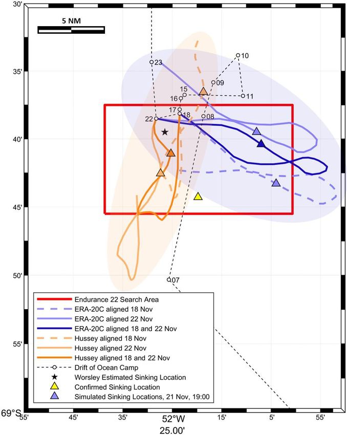
M. de Vos et al.: Drift of Endurance                                                                                              3

ber 1915. Further, it aims to reconstruct this unknown por-         downloaded on a regular grid with a resolution of 0.125◦
tion of the Endurance’s last days of drift using 20th century       (approximately 13.9 km). The interpolated product is pro-
meteorological reanalysis data and historical weather obser-        duced by ECMWF’s meteorological interpolation and re-
vations.                                                            gridding (MIR) package (Maciel et al., 2017) and is avail-
                                                                    able via ECMWF’s download portal at https://apps.ecmwf.
                                                                    int/datasets/data/era20c-daily/levtype=sfc/type=an/ (last ac-
2     Data and methods
                                                                    cess: 20 November 2022). Temporal resolution is 3-hourly.
2.1    Navigational fixes
                                                                    Data are produced by a modified version of an operational at-
                                                                    mospheric general circulation model (AGCM) and a data as-
Throughout the voyage, Captain Frank Worsley made esti-             similation scheme, which form the foundation of ECMWF’s
mates of position based on celestial sightings to track the         Integrated Forecast System (IFS). The IFS is normally used
movement of Endurance through the ice pack. Endurance               to produce short- and medium-term weather forecasts. Mod-
sank just before 17:00 LT (local time) on 21 November 1915.         ifications to the AGCM configuration and details regarding
The definition of “local time” is nuanced, but for this study       boundary conditions and forcing have been described in de-
may be considered approximately similar to UTC 3. Vari-             tail by Hersbach et al. (2015), who showed that the model
ations in the relationship between local time and UTC are           successfully reproduced low frequency variability of large-
negligible given the temporal resolution of the input data and      scale atmospheric features. The purpose of data assimilation
simulations used in this study. For a comprehensive explana-        during production of the reanalysis is to enhance the perfor-
tion of the derivation of local time and uncertainties thereof,     mance of the model in simulating weather events. The me-
the reader is referred to Bergman and Stuart (2018a, b). Bad        teorological observations of Hussey (see Sect. 2.3) have not
weather around the time of the sinking only allowed for nav-        been assimilated into the ERA-20C (Poli et al., 2016) reanal-
igational fixes 3 d before, and nearly a full day after the sink-   ysis dataset. As such, both datasets provide independent esti-
ing on 18 and 22 November 1915, respectively (Dowdeswell            mates of the actual synoptic situation during the time of En-
et al., 2020). The ship’s exact trajectory during the interven-     durance’s sinking. While the ERA-20C dataset comes with
ing approximately 4 d – referred to hereafter as the “target        large uncertainties, it has been shown to be capable of de-
period” – remains unknown. However, Worsley retrospec-              scribing the large-scale atmospheric circulation and by ex-
tively estimated the position of Ocean Camp on 21 Novem-            tension, should be able to describe the wind patterns in the
ber, assuming it to be offset by about 1.2 nautical miles to        western Weddell Sea. We extracted 10 m wind speeds and
the southeast of the 22 November position due to sea ice drift      directions from the ERA-20C dataset (Poli et al., 2016), ad-
(Bergman and Stuart, 2018b). We believe this estimate was           justed them to the 2 m vertical level by applying a logarith-
based on local wind observations, as Worsley had no means           mic profile correction (Manwell et al., 2009), and used them
by which to observe the sea ice drift directly. Dowdeswell          as a proxy to reconstruct the ice drift trajectory according to
et al. (2020) record that there are small uncertainties in the      the methodology in Sect. 2.4. ERA-20C winds for the tar-
positions of Ocean Camp and the Endurance due to factors            get period (along with mean sea level pressure) are shown
including: the fact that Captain Worsley made no astronomi-         in Fig. A1 (Appendix A1). For comparability, the 2 m level
cal observations between 3 d before and nearly 16 h after the       was selected as a best guess for the level at which Hussey’s
sinking because of bad weather; the drift of the chronometer        recordings were made (see Sect. 2.3) and a representative
used (primarily affecting longitude); the exact distance and        wind condition as experienced by the sea ice floes.
bearing between Ocean Camp (from where Worsley took a
fix) and the Endurance (whose position he estimated by off-         2.3   Meteorological observations
setting his Ocean Camp fix); and the speed and bearing of the
ice drift assumed for dead reckoning of the position. In this       To derive a further, independent estimate of ice drift during
work, we assume Worsley’s fixes to be accurate, and con-            the target period, we requested scans of the original log of the
centrate our analyses on uncertainties introduced by the ice        meteorological recordings and measurements made by the
drift.                                                              expedition meteorologist, Leonard Hussey, which are kept in
                                                                    the Archives of the Scott Polar Research Institute, University
2.2    ERA-20C reanalysis data
                                                                    of Cambridge. Hussey recorded surface meteorological vari-
                                                                    ables generally 4 times per day at 12:00, 16:00, 20:00, and
The ERA-20C (Poli et al., 2016) is a global reanalysis pro-         00:00 GMT. Among others, wind speed and direction were
duced by the European Centre for Medium-range Weather               measured using an anemometer and reported in units of the
Forecasts (ECMWF). It provides a range of atmospheric               Beaufort wind scale, and in cardinal and inter-cardinal direc-
and surface ocean variables with regular spatio-temporal            tions, respectively. These data were linearly interpolated to 3-
resolution for the period 1900–2010. Spatial resolution is          hourly resolution to match the ERA-20C data (see Sect. 2.2)
approximately 125 km on the native ERA-20C triangular               and then utilised to produce a drift trajectory for the target
grid (Poli et al., 2016). However, interpolated data were           period in the same way as for the ERA-20C data. It should

https://doi.org/10.5194/hgss-14-1-2023                                                    Hist. Geo Space Sci., 14, 1–13, 2023
4                                                                                             M. de Vos et al.: Drift of Endurance

be noted that no observations were taken during local night            – Case 1, using parameter values which both minimise
hours, leaving significant data gaps and introducing large un-           trajectory error and are well within realistic ranges.
certainties in reconstructed ice drift trajectories.
                                                                       – Case 2, using parameter values required to force the
                                                                         simulated sinking site to coincide with the actual sink-
                                                                         ing site.
2.4     Reconstructing ice drift trajectories
                                                                       – Case 3, using parameters with values more typical for
2.4.1     Description of sea ice drift                                   the Weddell Sea.
To construct the historical ice drift trajectories from both         Following Womack et al. (2022) and Nakayama et al. (2012),
datasets, we assumed a free drift regime, where sea ice mo-          since ocean forcing and internal ice stresses are neglected,
tion is purely described by wind forcing, and internal dy-           optimised wind factors and turning angles may differ from
namic forces and ocean forcing are neglected. This assump-           their real values due to their implicit inclusion of these ef-
tion has been shown to be reasonable over short timescales           fects. Whilst a likely scenario is identified, inferences about
for the Antarctic (Holland and Kwok, 2012; Kottmeier et              the unknown drift are drawn, acknowledging the range of
al., 1992; Kwok et al., 2017; Vihma et al., 1996; Martinson          possible outcomes within the envelope produced by the dif-
and Wamser, 1990), since wind is the primary forcing for sea         ferent configurations.
ice drift in the Weddell Sea (Uotila et al., 2000; Vihma and
Launiainen, 1993; Vihma et al., 1996). It should be noted            2.4.2    Implementation
that caution is required when applying this assumption in the
Arctic, where internal ice stress, Coriolis force (due to gen-       For each 3-hourly time step, the future position of the virtual
erally thicker ice), and geographical constraints are likely to      sea ice floe is predicted by applying the wind-driven drift dis-
exert more control on the drift of sea ice (Lepparanta, 2011;        tance and direction to the Vincenty formula (Vincenty, 1975),
Martinson and Wamser, 1990). Notwithstanding, free drift             as implemented in MATLAB by Pawlowicz (2020). Figure 2
has been shown to be applicable in certain Arctic cases (e.g.        shows the resulting trajectories. A series of simulations us-
Cole et al., 2014; Park and Stewart, 2016). The assumption           ing different wind factors and turning angles were performed
may also break down near the coast or in mostly open wa-             (Fig. A2). The effects of changing wind factors and turning
ter, where internal ice stress and ocean currents, respectively,     angles on the resulting distance between the simulated and
reduce the dependence on wind drift (Uotila, 2001). Further,         actual sinking sites can be seen by comparing correspond-
free drift parameters; namely, sea ice drift speed as a pro-         ing trajectories in Figs. 2 and A3–A4 (Appendix A1). These
portion of wind speed (hereafter wind factor; Nakayama et            results guided the selection of cases described in Sect. 2.4.1.
al., 2012) and the angle between the wind and sea ice drift
vectors (hereafter turning angle; Doble and Wadhams, 2006)           2.5     Trajectory alignment and nudging
vary widely, even within similar time and places (Kottmeier
et al., 1992), and are an important control on the drift of sea      None of the reconstructed trajectories are able to link Wors-
ice. This variability is reflected in the empirical derivations of   ley’s fix on 18 November to his 22 November fix. While this
wind factors and turnings angles in the literature. Recently,        could be due to errors in Worsley’s navigation, we assume
Womack et al. (2022) determined wind factors ranging from            that it is mainly caused by errors in the wind forcing datasets.
1– 6 % (mean 2.73 %) and tuning angles ranging from −50–             To overcome this limitation, we provide two additional ver-
50◦ (mean −19.83◦ ) for an area of the Antarctic marginal            sions of a corrected trajectory in addition to the default. For
ice zone east of the study domain. In the Weddell Sea, a vast        each of Cases 1–3, we therefore provide three possible tra-
range of parameter values is reported, with wind factors of          jectories:
1.5–3.5 % (e.g. Kottmeier and Sellmann, 1996; Kottmeier et            1. The default trajectory (dashed lines in Fig. 2), which
al., 1992; Vihma and Launiainen, 1993; Uotila et al., 2000;              begins and develops naturally from Worsley’s fix of
Martinson and Wamser, 1990) and turning angles of −20                    18 November.
to 60◦ (Uotila et al., 2000; Womack et al., 2022). Reported
mean values are typically 2–3 % and −20–−30◦ , with an ac-            2. A “nudged” trajectory leading from Worsley’s
knowledgement of the spread and scattering of data points.               18 November fix to his 22 November fix. To achieve
   For in-depth discussions of the free drift assumption and             this, the simulated trajectory was co-located in the
its parameters, which is beyond the scope of this study, the             start point on 18 November, and the averaged position
reader is referred to the literature cited in this section. Inso-        offset for each time step added in such a way that the
far as free drift parameter value selection affects our results,         simulated position on 22 November matches Worsley’s
our strategy is to apply the free drift solution to our problem          observation (dark orange and dark blue solid lines in
using a range of realistic parameter values. In summary, we              Fig. 2) This corresponds to a purely time-dependent
present three selected cases:                                            accumulating error.

Hist. Geo Space Sci., 14, 1–13, 2023                                                     https://doi.org/10.5194/hgss-14-1-2023
M. de Vos et al.: Drift of Endurance                                                                                                         5

Figure 2. Case 1 reconstructed drift tracks and sinking sites using ERA-20C reanalysis (blue) and Hussy’s meteorological observations
(orange). Case 1 utilised a wind factor of 1.75 % and a turning angle of 0◦ . Coloured ellipses show approximate uncertainty regions associated
with the respective dataset.

  3. A further alternative trajectory, nudged to align with               3     Results and discussion
     Worsley’s fix on 22 November only, without chang-
     ing its general shape. This accounts for the possibility             3.1    Estimating ERA-20C drift prediction error
     that the fix of 22 November is more accurate than the
     18 November fix (light orange and light blue solid lines             To assess the relative uncertainty of the ERA-20C drift pre-
     in Fig. 2).                                                          dictions in a more general sense (than only for the target pe-
                                                                          riod), we performed a basic assessment of mean predicted
Assessing the extremities described by each set of three tra-             position error. Positions predicted by applying ERA-20C
jectories allows us to estimate roughly the magnitude of posi-            near-surface winds to virtual ice floes were reconstructed for
tion uncertainty associated with sea ice drift (see orange and            the period 18 January until 21 November 1915, during which
blue ellipses in Fig. 2).                                                 Endurance was beset and drifting in the ice pack. The error is
                                                                          an average for the periods between positional fixes made by
                                                                          Worsley. The drift of virtual ice floes (defined by the naviga-
                                                                          tional fixes) is simulated according to the method described

https://doi.org/10.5194/hgss-14-1-2023                                                            Hist. Geo Space Sci., 14, 1–13, 2023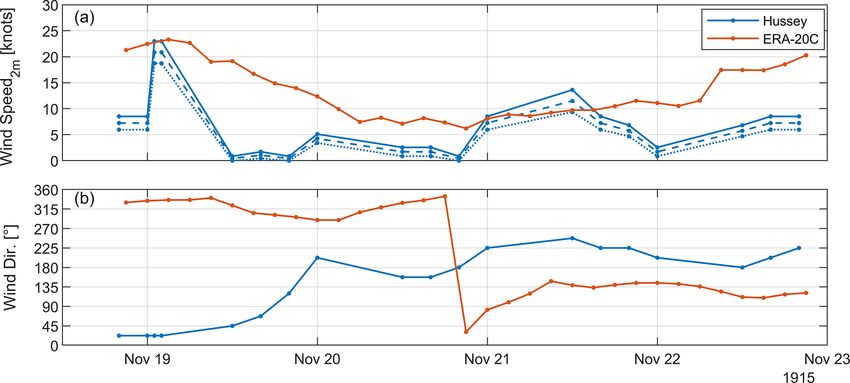
6                                                                                          M. de Vos et al.: Drift of Endurance

in Sect. 2.4.2, by using ERA-20C winds and wind factors and       to Hussey’s observation of a much faster speed drop fol-
turning angles as used in simulation Cases 1–3. After sensi-      lowing the strong northerlies (ERA winds stay stronger for
tivity testing, these were decided to be as follows:              longer and never drop quite as low as Hussey’s recordings).
                                                                  The second is a significant discrepancy from the afternoon of
    – Case 1 with a wind factor of 1.75 % and turning angle       21 November until the end of the period. Whilst both datasets
      of 0◦ ,                                                     suggest winds of around 10 knots by the afternoon of the
                                                                  21st, Hussey’s observed gradual increase to the end of the
    – Case 2 with a wind factor of 1.85 % and turning angle
                                                                  period is preceded by an initial drop to below 5 knots. ERA
      of 17.5◦ ,
                                                                  does not produce this decrease, so whilst it shows a similar
    – Case 3 with a wind factor of 2.5 % and turning angle of     gradual increase through the end of the period, a discrepancy
      −25◦ ,                                                      of 5–10 knots persists.

where a negative turning angle implies a deviation to the         3.3   Reconstructed trajectories and sinking sites
left of the wind. Whenever a position update from Worsley’s
log becomes available, the end position is automatically cor-     For all three cases (which vary by wind factor and turning an-
rected, such that the initial position for the next drift step    gle) using ERA-20C winds, the default trajectories (i.e. those
is Worsley’s most recent fix. Mean error is computed as the       starting at the 18 November position, indicated by dashed
mean of the distances between the end position from the fore-     lines in Fig. 2) yield the shortest distance between simulated
cast and the corresponding end positions available in Wors-       and actual sinking sites (i.e. nudging the trajectories, as ex-
ley’s log. Figure 3 shows the histogram of all position errors    plained in Sect. 2.5, did not improve simulated sinking lo-
for the period during which Endurance was beset and drifting      cations). Distances between the simulated and actual sinking
in the pack ice. For Cases 1, 2, and 3 (representing different    locations for Cases 1–3 along these trajectories are 3.5, 0.0,
wind factor/turning angle combinations), mean position dif-       and 10.8 km, respectively. These simulated sinking locations
ferences (i.e. the distance between simulated positions and       are consistently north (by 1.7, 0.0, and 1.8 km) and east (by
Worsley’s fixes) were 13.4, 14.0, and 15.4 km, respectively.      3.0, 0.00, and 10.6 km) of the actual site.
Median position differences were 10.7, 11.0, and 12.0 km,            Using Hussey’s winds, Case 1 and 2 sinking locations
respectively. Case 1 produces the lowest mean and median          are closest to the actual one when their trajectories are
differences, though the cases produce generally similar error     nudged to match both the 18 and 22 November positions.
distributions.                                                    For Case 3, nudging to 22 November produces the best result.
                                                                  Distances between the simulated and actual sinking locations
3.2    Comparison of ERA-20C winds with Hussey
                                                                  for Cases 1–3 along the abovementioned trajectories are 0.3,
       observations
                                                                  10.1, and 7.0 km, respectively. Case 1’s simulated sinking lo-
                                                                  cation is north (by 7.4 km) and east (by 5.6 km) of the actual
Figure 4 shows a comparison between Hussey’s wind record-         location, whilst Cases 2 and 3’s simulated sinking locations
ings and the ERA-20C wind data. Whilst there are broad            are north (by 7.6 and 5.9 km) and west (by 6.7 and 3.7 km)
similarities between the two datasets, there are differences in   of the actual location.
speed, direction, and timing, which account for material dif-        All simulations, regardless of wind input data or parame-
ferences in corresponding trajectories. Broadly, both datasets    ter values, produce sinking locations with southerly compo-
suggest strong north-component winds at the start of the tar-     nent offsets from Worsley’s estimate (consistent with the ac-
get period, which weaken and veer to become light south-          tual sinking location) and northerly component offsets from
component winds and increase in strength slightly by the          the actual location (suggesting that with the exception of the
end of the period. Concerning changes in direction, however,      idealised case, they do not quite capture the extent of the
Hussey observed an earlier and more gradual veering from          southerly excursion). These results, among others, are sum-
northerly winds (to southerlies by the start of 20 Novem-         marised in Table 1.
ber) than ERA, which suggests winds veered later and more            Within realistic parameter value ranges, applying ERA-
suddenly to become south–southeasterly by mid-morning             20C to the drift simulation yields closer estimates of the sink-
on 21 November. Thereafter, Hussey’s recordings indicate          ing location. Though we are unable to say for sure, we deem
winds remained roughly south–southwesterly until the end          Case 1 (Fig. 2) to be the most likely, given that its parame-
of the period, with southerly and south–southeasterly varia-      ter values are well within realistic ranges and result in the
tions for short periods. ERA winds remained more uniformly        lowest mean and median error for the overall drift trajec-
southeasterly until the end of the period. Concerning speeds,     tory (January–November; Fig. 3). In this case, a simulated
whilst both datasets agree on generally high speeds, followed     sinking location some 3.5 km (1.7 km south, 3.0 km east) of
by a decrease and then an increase, there are two principal       the actual location is produced. In Case 2 (idealised case,
discrepancies. The first is a significant difference between      Fig. A3), where the simulated sinking location is forced to
the mornings of 19 and 20 November (up to 20 knots) due           coincide with the actual location, parameter values are still

Hist. Geo Space Sci., 14, 1–13, 2023                                                  https://doi.org/10.5194/hgss-14-1-2023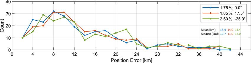
M. de Vos et al.: Drift of Endurance                                                                                                            7

Figure 3. Distribution of errors for predicted positions using initial positions from Worsley’s navigational fixes and simulated ERA-20C
surface wind-driven drift. The computation is for the period 18 January–21 November 1915; the time during which Endurance was beset
and drifting with the sea ice. The three sensitivity test cases discussed in Sect. 3.4 are presented (for each case, the legend refers to the wind
factor and the turning angle). Also presented are mean and median errors.

Figure 4. Time series comparison of wind speeds (a and directions (b) between recordings from Hussey and the ERA-20C product. For
the Hussey wind speeds (since Hussey reported Beaufort indices), the solid (dotted) line indicates wind speeds corresponding to the upper
(lower) Beaufort index bound. The dashed line shows the mean for that index.

within realistic ranges, as reported in the literature (1.85 %             it does not produce very realistic sinking locations. It also
and 17.5◦ ), but further from their typical average values. To             produces higher mean and median error than Cases 1 and 2.
achieve the same using Hussey’s observations, unrealistic pa-                 For ERA-20C Case 1, the principal axis of uncertainty
rameter values are required (wind factors < 3.8 % and turn-                runs north–northeast to south–southeast (∼ 140◦ ). This is the
ing angles < −48◦ ), which at the same time cause the corre-               same for Case 2 (idealised case; ∼ 155◦ ) and east–southeast
sponding ERA-20C simulations to be completely degraded                     for Case 3 (∼ 122◦ ). It is interesting to note that for many
(whereas for values optimised for ERA-20C, the Hussy re-                   of the simulations, meridional, and zonal offsets of sinking
sults remain within the search area). This suggests ERA-20C                locations (representative of uncertainty in sea ice drift) are of
wind inputs and resulting trajectories are more reliable.                  the same order of magnitude as those associated with Wors-
   In terms of the shape of the trajectory, all ERA-20C tra-               ley’s traditional navigation methods, as analysed in detail by
jectories agree on a southeasterly excursion, followed by a                Bergman and Stuart (2018b). In some cases, they are nearly
clockwise turn to the northwest prior to sinking. If Case 1                double.
is the most likely and Case 2 is the idealised case, we deem
Case 3 (Fig. A4) a possible but relatively unlikely scenario.
Acknowledging how widely parameter values vary, Case 3 is                  3.4    Accounting for discrepancies
presented since it uses very typical, average values from the
                                                                           The accuracy of trajectories, as simulated in this study via
literature (wind factor 2.5 %, turning angle −25◦ ). However,
                                                                           a simplified free drift method, depend on three main fac-
                                                                           tors: the start points, the quality (resolution and accuracy)

https://doi.org/10.5194/hgss-14-1-2023                                                              Hist. Geo Space Sci., 14, 1–13, 2023
8 M. de Vos et al.: Drift of Endurance
Table 1. Total and vector component distances from the various simulated sinking locations to the actual sinking locations as well as to
Worsley’s estimated sinking location. Negative meridional (zonal) values indicate offsets to the south (west) of the reference.
Case Trajectory Distance from actual sinking Distance from Worsley’s estimated)
location (km) sinking location (km)
Total Meridional Zonal Total Meridional Zonal
ERA-20C 1 Default (18 November) 3.5 1.7 3.0 10.3 −7.1 7.5
2 Default (18 November) 0.0 0.0 0.0 9.9 −8.8 4.5
3 Default (18 November) 10.8 1.8 10.6 16.7 −7.0 15.2
Hussey 1 Nudged (18 and 22 November) 9.3 7.4 5.6 1.9 −1.5 −1.1
2 Nudged (18 and 22 November) 10.1 7.6 −6.7 2.6 −1.3 −2.2
3 Nudged (22 November) 7.0 6.0 −3.7 5.7 −5.6 −0.6
of the wind data, and the selection of free drift parameter ing and gusty winds can cause the unpredictable breakup of
values (though the latter two are probably more consequen- sea ice, which might explain both the shift in ice conditions
tial). Since none of these are known with absolute certainty, which catalysed the sinking of the vessel and the breakdown
the problem of reconstructing Endurance’s trajectory is fun- of the free drift assumption (e.g. Nicolaus et al., 2022).
damentally under-constrained. Imposing assumptions allows Whilst this sort of experimentation certainly yields insight,
us to close the problem and draw inferences about the likely the selection of constraints and assumptions ultimately re-
state of the other factors. mains, to a certain extent, subjective.
If we assume the wind input data are perfect, remaining
discrepancies between the simulated and actual sinking loca- 4 Conclusions
tions (and, by extension, errors in the shape of the associated
trajectory) are likely due to the inaccuracy of the parameter This study demonstrates the potential of modern reanalysis
values we impose (using, for example, values from the liter- weather models to help reconstruct possible ice drift trajec-
ature), which themselves depend on a host of factors. As a tories of Shackleton’s Endurance and for use in marine ar-
basic example, the more compact and thicker the sea ice, the chaeological projects more generally.
larger the turning angle (Uotila et al., 2000; Martinson and Whilst the prescription of a definitive trajectory is pre-
Wamser, 1990) and the rougher the floe, the greater the wind cluded by the sensitivity of simulations to choices of parame-
factor (Kottmeier et al., 1992). This is information we do not ter values and potential inaccuracies of the wind data, a likely
have. scenario was uncovered based on an envelope of results and
Alternatively, if we force the parameter values to be “cor- consistent features therein.
rect” (that is, tune the simulation to produce the correct sink- Specifically, we showed that between 18 and 22 Novem-
ing location as in ERA-20C Case 2), we may end up with ber, Endurance likely followed a southeasterly excursion,
values near their probable limits (or at least, more unusual followed by an anticlockwise turn and a short period of
according to the literature). In this case, discrepancies be- north–westward drift, prior to sinking, which is not described
tween the imposed values and those we might have expected in Worsley’s navigational data. The southerly excursion may
based on literature could be due to their needing to include, have taken Endurance further south than the latitude at which
implicitly, effects not explicitly accounted for (e.g. internal the vessel was ultimately found.
ice stress and ocean currents), or to inaccuracies of the wind We conclude that rigorous analysis of available weather
data. For example, in Case 2, the perfect sinking location is and sea ice drift data is important to marine archaeological
produced by a wind factor of 1.85 % and a turning angle of projects in sea ice-covered oceans. This is not only true for
17.5◦ . Whilst these are within empirical ranges, turning an- proper positioning of the drifting survey vessel in the ice,
gles in the Weddell Sea are more usually negative (i.e. to the but also for understanding the implications of sea ice drift on
left of the wind). It is possible that the turning angle of 17.5◦ the position and trajectory of historic vessels locked in the
is required to mask an anticlockwise directional bias in the ice. In this particular case, uncertainty due to the drift of sea
wind dataset of ∼ 37.5◦ . In that case, the true turning angle ice was at least as large, and in many cases, larger than the
becomes −20◦ , which would be very typical. Rapid changes uncertainty associated with navigational fixes.
in near-surface winds are often poorly reproduced by models,
and since Endurance sank after the passage of a cyclone, it’s
possible that this is the case. Moreover, such rapidly chang-
Hist. Geo Space Sci., 14, 1–13, 2023 https://doi.org/10.5194/hgss-14-1-2023M. de Vos et al.: Drift of Endurance 9 Appendix A: Figure A1. Six-hourly maps of wind speed (colour scale, vector magnitude) and direction (vector orientation) and mean sea level pressure (contours) from ERA-20C. Also shown (white) are the search box and ERA-20C simulated trajectory. All dates refer to 1915. https://doi.org/10.5194/hgss-14-1-2023 Hist. Geo Space Sci., 14, 1–13, 2023
10                                                                                                   M. de Vos et al.: Drift of Endurance

Figure A2. Distance between ERA-20C simulated and actual sinking sites as a function of wind factor (a) and turning angle (b). These
sensitivity results were used to arrive at the optimised parameter values for simulation Case 1 and the idealised values for Case 2.

Figure A3. Case 2 reconstructed drift tracks and sinking sites using ERA-20C reanalysis (blue) and Hussy’s meteorological observations
(orange). Case 2 is an idealised case, where the ERA-20C simulated sinking position is forced to coincide with the actual sinking location by
adjusting model parameter values (note the coincident sinking location triangles). The required parameters are a wind factor of 1.85 % and a
turning angle of 17.5◦ . Coloured ellipses show approximate uncertainty regions associated with the respective dataset.

Hist. Geo Space Sci., 14, 1–13, 2023                                                            https://doi.org/10.5194/hgss-14-1-2023
M. de Vos et al.: Drift of Endurance                                                                                                    11

Figure A4. Case 3 reconstructed drift tracks and sinking sites using ERA-20C reanalysis (blue) and Hussy’s meteorological observations
(orange). Case 3 utilised a wind drift factor of 2.5 % and a turning angle of −25◦ . Coloured ellipses show approximate uncertainty regions
associated with the respective dataset.

Data availability. ERA-20C data are freely available at ECMWF           Author contributions. Conceptualisation: MdV; data curation:
(https://www.ecmwf.int/en/forecasts/datasets/reanalysis-datasets/       MdV, CK, PK, JS; formal analysis: MdV, PK, CK; investigation:
era-20c, last access: 20 November 2022). Leonard Hussey’s meteo-        MdV, PK, CK, LR, JS; methodology: MdV, CK, LR, PK; Project
rological observations and Reginald James’s diary (from which the       administration: MdV, CK, LR, JS; resources: MdV, LR, PK; soft-
drift track was compiled) are available upon request of the Archives    ware: MdV, CK, PK, MS; Supervision: MdV, JS, LR; Validation:
of the Scott Polar Research Institute, University of Cambridge,         CK, MdV; Visualisation: MdV, CK, MS; writing – original draft
with references GB 15 DR LEONARD HUSSEY/IMPERIAL                        preparation: MdV, CK; writing – review and editing: all authors.
TRANS-ANTARCTIC EXPEDITION [WEDDELL SEA PARTY]:
MS 1605/2/1; D Meteorological Returns, weather diary, January
1915 to December 1915 [Weddell Sea]), and GB 15 REGINALD                Competing interests. The contact author has declared that none
WILLIAM JAMES, respectively.                                            of the authors has any competing interests.

https://doi.org/10.5194/hgss-14-1-2023                                                         Hist. Geo Space Sci., 14, 1–13, 2023
12                                                                                                 M. de Vos et al.: Drift of Endurance

Disclaimer. Publisher’s note: Copernicus Publications remains           Kottmeier, C. and Sellmann, L.: Atmospheric and oceanic forcing of
neutral with regard to jurisdictional claims in published maps and        Weddell Sea ice motion, J. Geophys. Res.-Oceans, 101, 20809–
institutional affiliations.                                               20824, https://doi.org/10.1029/96JC01293, 1996.
                                                                        Kottmeier, C., Olf, J., Frieden, W., and Roth, R.: Wind forcing
                                                                          and ice motion in the Weddell Sea region, J. Geophys. Res., 97,
Acknowledgements. The authors would like to thank the follow-             20373–20383, https://doi.org/10.1029/92jd02171, 1992.
ing. The Falklands Maritime Heritage Trust for conceptualising and      Kwok, R., Pang, S. S., and Kacimi, S.: Sea ice drift in the Southern
enabling this expedition and our participation in it; Director of Ex-     Ocean: Regional patterns, variability, and trends, Elementa, 5,
ploration for Endurance22, Mensun Bound, for encouraging the au-          32, https://doi.org/10.1525/elementa.226, 2017.
thors to publish our research; Naomi Boneham at the Archives of         Lepparanta, M.: The drift of sea ice, 2nd edn., Springer
the Scott Polar Research Institute, University of Cambridge, for the      Science & Business Media, Chichester, 347 pp.,
short-notice provision of Hussey’s original meteorological records        https://doi.org/10.1007/978-3-642-04683-4, 2011.
while we were at sea; Julian Dowdeswell and Toby Benham for the         Maciel, P., Quintino, T., Modigliani, U., Dando, P., Raoult, B., De-
provision of the digitised Endurance drift track, and Chairman of the     coninck, W., Rathgeber, F., and Simarro, C.: The new ECMWF
Falklands Maritime Heritage Trust Donald Lamont and Director of           interpolation package MIR, ECMWF Newsletter no. 152, 36–39,
Endurance22 Subsea Operations, Nico Vincent, for their valuable           https://doi.org/10.21957/h20rz8, 2017.
input to our manuscript.                                                Manwell, J., McGowan, J., and Rogers, A.: Wind energy explained:
                                                                          theory, design, and application, 2nd edn., John Wiley & Sons
                                                                          Ltd., Chichester, 704 pp., ISBN: 978-0-470-01500-1, 2009.
Review statement. This paper was edited by Kevin Hamilton and           Martinson, D. G. and Wamser, C.: Ice drift and momentum ex-
reviewed by two anonymous referees.                                       change in winter Antarctic pack ice, J. Geophys. Res.-Oceans,
                                                                          95, 1741–1755, https://doi.org/10.1029/jc095ic02p01741, 1990.
                                                                        Nakayama, Y., Ohshima, K. I., and Fukamachi, Y.: Enhance-
                                                                          ment of sea ice drift due to the dynamical interaction between
References                                                                sea ice and a coastal ocean, J. Phys. Oceanogr., 42, 179–192,
                                                                          https://doi.org/10.1175/JPO-D-11-018.1, 2012.
Bergman, L. and Stuart, R.: Navigation of the Shackleton Expe-          Nicolaus, M., Perovich, D. K., Spreen, G., Granskog, M. A., von
  dition on the Weddell Sea pack ice, Records of the Canterbury           Albedyll, L., Angelopoulos, M., Anhaus, P., Arndt, S., Jakob
  Museum, 32, 67–98, 2018a.                                               Belter, H., Bessonov, V., Birnbaum, G., Brauchle, J., Calmer,
Bergman, L. and Stuart, R. G.: On the Location of Shack-                  R., Cardellach, E., Cheng, B., Clemens-Sewall, D., Dadic, R.,
  leton’s Vessel Endurance, J. Navigation, 72, 307–320,                   Damm, E., de Boer, G., Demir, O., Dethloff, K., Divine, D. v.,
  https://doi.org/10.1017/S0373463318000619, 2018b.                       Fong, A. A., Fons, S., Frey, M. M., Fuchs, N., Gabarró, C., Ger-
Cole, S. T., Timmermans, M. L., Toole, J. M., Krishfield, R. A., and      land, S., Goessling, H. F., Gradinger, R., Haapala, J., Haas, C.,
  Thwaites, F. T.: Ekman veering, internal waves, and turbulence          Hamilton, J., Hannula, H. R., Hendricks, S., Herber, A., Heuzé,
  observed under arctic sea ice, J. Phys. Oceanogr., 44, 1306–1328,       C., Hoppmann, M., Høyland, K. V., Huntemann, M., Hutch-
  https://doi.org/10.1175/JPO-D-12-0191.1, 2014.                          ings, J. K., Hwang, B., Itkin, P., Jacobi, H. W., Jaggi, M., Ju-
Doble, M. J. and Wadhams, P.: Dynamical contrasts be-                     tila, A., Kaleschke, L., Katlein, C., Kolabutin, N., Krampe, D.,
  tween pancake and pack ice, investigated with a drift-                  Kristensen, S. S., Krumpen, T., Kurtz, N., Lampert, A., Lange,
  ing buoy array, J. Geophys. Res.-Oceans, 111, C11S24,                   B. A., Lei, R., Light, B., Linhardt, F., Liston, G. E., Loose, B.,
  https://doi.org/10.1029/2005JC003320, 2006.                             Macfarlane, A. R., Mahmud, M., Matero, I. O., Maus, S., Mor-
Dowdeswell, J. A., Batchelor, C. L., Dorschel, B., Benham, T.             genstern, A., Naderpour, R., Nandan, V., Niubom, A., Oggier,
  J., Christie, F. D. W., Dowdeswell, E. K., Montelli, A., Arndt,         M., Oppelt, N., Pätzold, F., Perron, C., Petrovsky, T., Pirazzini,
  J. E., and Gebhardt, C.: Sea-floor and sea-ice conditions in            R., Polashenski, C., Rabe, B., Raphael, I. A., Regnery, J., Rex,
  the western Weddell Sea, Antarctica, around the wreck of Sir            M., Ricker, R., Riemann-Campe, K., Rinke, A., Rohde, J., Sal-
  Ernest Shackleton’s Endurance, Antarct. Sci., 32, 301–313,              ganik, E., Scharien, R. K., Schiller, M., Schneebeli, M., Semm-
  https://doi.org/10.1017/S0954102020000103, 2020.                        ling, M., Shimanchuk, E., Shupe, M. D., Smith, M. M., Smolyan-
ECMWF: ERA-20C, ECMWF [data set], https://www.ecmwf.                      itsky, V., Sokolov, V., Stanton, T., Stroeve, J., Thielke, L., Tim-
  int/en/forecasts/datasets/reanalysis-datasets/era-20c, last access:     ofeeva, A., Tonboe, R. T., Tavri, A., Tsamados, M., Wagner, D.
  20 November 2022.                                                       N., Watkins, D., Webster, M., and Wendisch, M.: Overview of the
Gilbert, N.: Endurance 22 Initial Environmental Evaluation,               MOSAiC expedition: Snow and sea ice, Elementa, 10, 000046,
  Christchurch,           https://endurance22.org/uploads/2022/01/        https://doi.org/10.1525/elementa.2021.000046, 2022.
  Endurance22_IEE.pdf (last access: 21 December 2022),                  Park, H.-S. and Stewart, A. L.: An analytical model for wind-
  2021.                                                                   driven Arctic summer sea ice drift, The Cryosphere, 10, 227–
Hersbach, H., Peubey, C., Simmons, A., Berrisford, P., Poli, P.,          244, https://doi.org/10.5194/tc-10-227-2016, 2016.
  and Dee, D.: ERA-20CM: A twentieth-century atmospheric                Pawlowicz, R.: M_Map: A mapping package for MATLAB, version
  model ensemble, Q. J. Roy. Meteor. Soc., 141, 2350–2375,                1.4m, EOAS UBC [software], https://www.eoas.ubc.ca/~rich/
  https://doi.org/10.1002/qj.2528, 2015.                                  map.html (last access: 31 November 2022), 2020.
Holland, P. R. and Kwok, R.: Wind-driven trends in                      Poli, P., Hersbach, H., Dee, D. P., Berrisford, P., Simmons, A. J., Vi-
  Antarctic sea-ice drift, Nat. Geosci., 5, 872–875,                      tart, F., Laloyaux, P., Tan, D. G. H., Peubey, C., Thépaut, J., Tré-
  https://doi.org/10.1038/ngeo1627, 2012.

Hist. Geo Space Sci., 14, 1–13, 2023                                                          https://doi.org/10.5194/hgss-14-1-2023
M. de Vos et al.: Drift of Endurance 13 molet, Y., Hólm, E. V., Bonavita, M., Isaksen, L., and Fisher, M.: Uotila, J., Vihma, T., and Launiainen, J.: Response of the Wed- ERA-20C: An Atmospheric Reanalysis of the Twentieth Cen- dell Sea pack ice to wind forcing, J. Geophys. Res.-Oceans, 105, tury, J. Climate, 29, 4083–4097, https://doi.org/10.1175/JCLI-D- 1135–1151, https://doi.org/10.1029/1999jc900265, 2000. 15-0556.1, 2016. Vihma, T. and Launiainen, J.: Ice drift in the Weddell Sea in 1990– Rabenstein, L. (Ed.): Endurance22, Cruise Scientific Report, 1–95, 1991 as tracked by a satellite buoy, J. Geophys. Res., 98, 14471– https://endurance22.org/uploads/2022/06/Science_Report_ 14485, https://doi.org/10.1029/93jc00649, 1993. Endurance22_final_version.pdf (last access: 3 January 2023), Vihma, T., Launiainen, J., and Uotila, J.: Weddell Sea ice drift: 2022. Kinematics and wind forcing, J. Geophys. Res.-Oceans, 101, Shackleton, E. H.: South: The Story of Shackleton’s Last Expe- 18279–18296, https://doi.org/10.1029/96JC01441, 1996. dition 1914–1917, MacMillan, New York, 380 pp., https://nrs. Vincenty, T.: Direct and inverse solutions of geodesics on the ellip- lib.harvard.edu/urn-3:fhcl:1273490 (last access: 20 December soid with application of nested equations, Surv. Rev., 23, 88–93, 2022), 1920. https://doi.org/10.1179/sre.1975.23.176.88, 1975. Shears, J., Dowdeswell, J., Ligthelm, F., and Wachter, P.: Womack, A., Vichi, M., Alberello, A., and Toffoli, A.: Atmo- The Weddell Sea Expedition 2019, EGU General As- spheric drivers of a winter-to-spring Lagrangian sea-ice drift in sembly 2020, Online, 4–8 May 2020, EGU2020-21896, the Eastern Antarctic marginal ice zone, J. Glaciol., 68, 999– https://doi.org/10.5194/egusphere-egu2020-21896, 2020. 1013, https://doi.org/10.1017/jog.2022.14, 2022. Uotila, J.: Observed and modelled sea-ice drift response to wind forcing in the northern Baltic Sea, Tellus A, 53, 112–128, 2001. https://doi.org/10.5194/hgss-14-1-2023 Hist. Geo Space Sci., 14, 1–13, 2023
You can also read