Uncertainty quantification for epidemiological forecasts of COVID-19 through combinations of model predictions
←
→
Page content transcription
If your browser does not render page correctly, please read the page content below
Content includes material subject to © Crown copyright (2021), Dstl. This material is licensed under the terms of the Open Government Licence
                                           except where otherwise stated. To view this licence, visit http://www.nationalarchives.gov.uk/doc/open-government-licence/version/3 or write to
                                           the Information Policy Team, The National Archives, Kew, London TW9 4DU, or email: psi@nationalarchives.gov.uk.

                                                    Uncertainty quantification for epidemiological forecasts of
                                                     COVID-19 through combinations of model predictions
arXiv:2006.10714v3 [stat.AP] 12 Aug 2021

                                                        D. S. Silk† , V. E. Bowman† , D. Semochkina‡ , U. Dalrymple† and D. C. Woods‡
                                                                  † Defence Science and Technology Laboratory, Porton Down
                                                              ‡ Statistical Sciences Research Institute, University of Southampton

                                                                                                       August 13, 2021

                                               Scientific advice to the UK government throughout the COVID-19 pandemic has been informed by ensembles
                                           of epidemiological models provided by members of the Scientific Pandemic Influenza group on Modelling (SPI-M).
                                           Among other applications, the model ensembles have been used to forecast daily incidence, deaths and hospitaliza-
                                           tions. The models differ in approach (e.g. deterministic or agent-based) and in assumptions made about the disease and
                                           population. These differences capture genuine uncertainty in the understanding of disease dynamics and in the choice
                                           of simplifying assumptions underpinning the model. Although analyses of multi-model ensembles can be logistically
                                           challenging when time-frames are short, accounting for structural uncertainty can improve accuracy and reduce the
                                           risk of over-confidence in predictions. In this study, we compare the performance of various ensemble methods to
                                           combine short-term (14 day) COVID-19 forecasts within the context of the pandemic response. We address practical
                                           issues around the availability of model predictions and make some initial proposals to address the short-comings of
                                           standard methods in this challenging situation.

                                           1     Introduction
                                           Comprehensive uncertainty quantification in epidemiological modelling is a timely and challenging problem. During
                                           the COVID-19 pandemic, a common requirement has been statistical forecasting in the presence of an ensemble of
                                           multiple candidate models. For example, multiple candidate models may be available to predict disease case numbers,
                                           resulting from different modelling approaches (e.g. mechanistic or empirical) or differing assumptions about spatial or
                                           age mixing. Alternative models capture genuine uncertainty in scientific understanding of disease dynamics, different
                                           simplifying assumptions underpinning each model derivation, and/or different approaches to the estimation of model
                                           parameters. While the analysis of multi-model ensembles can be computationally challenging, accounting for this
                                           ‘structural uncertainty’ can improve forecast accuracy and reduce the risk of over-confident prediction [1,2] .
                                                A common ensemble approach is model averaging, which tries to find an optimal combination of models in the
                                           space spanned by all individual models [3,4] . However, in many settings this approach can fail dramatically: (i) the re-
                                           quired marginal likelihoods (or equivalently Bayes factors) can depend on arbitrary specifications for non-informative
                                           prior distributions of model-specific parameters; and (ii) asymptotically the posterior model probabilities, used to
                                           weight predictions from different models, converge to unity on the model closest to the ‘truth’. While this second
                                           feature may be desirable when the set of models under consideration contains the true model (the M-closed setting), it
                                           is less desirable in more realistic cases when the model set does not contain the true data generator (M-complete and
                                           M-open). Here, this property of Bayesian model averaging asymptotically choosing a single model can be thought of
                                           as a form of overfitting. For these latter settings, alternative methods of combining predictions from model ensembles
                                           may be preferred, for example, via combinations of individual predictive densities [5] . Combination weights can be
                                           chosen via application of predictive scoring, as commonly applied in meteorological and economic forecasting [6,7] .
                                                If access to full posterior information is available, other approaches are also possible. Model stacking methods [8] ,
                                           see Section 2.2, can be applied directly, ideally using leave-one-out predictions or sequential predictions of future

                                                                                                                  1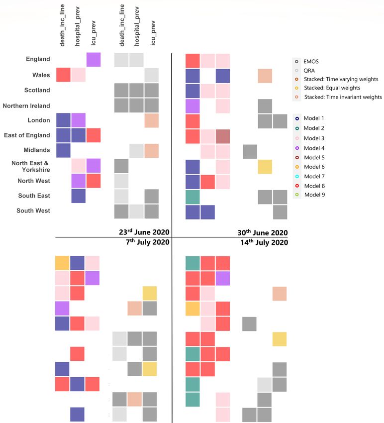
Content includes material subject to © Crown copyright (2021), Dstl. This material is licensed under the terms of the Open Government Licence
except where otherwise stated. To view this licence, visit http://www.nationalarchives.gov.uk/doc/open-government-licence/version/3 or write to
the Information Policy Team, The National Archives, Kew, London TW9 4DU, or email: psi@nationalarchives.gov.uk.

data to mitigate over-fitting. Alternatively, the perhaps confusingly named Bayesian model combination method [9,10]
could be employed, where the ensemble is expanded to include linear combinations of the available models. For
computationally expensive models, where straightforward generation of predictive densities is prohibitive, a statistical
emulator built from a Gaussian process priors [11] could be assumed for each expensive model. Stacking or model
combination can then be applied to the resulting posterior predictive distributions, conditioning on model runs and
data.
    In this paper we explore the process of combining short-term epidemiological forecasts for COVID-19 daily deaths,
and hospital and intensive care unit (ICU) occupancy, within the context of supporting UK decision makers during
the pandemic response. In practice, this context placed constraints on the information available to the combination
algorithms. In particular, the individual model posterior distributions were unavailable, which prohibited the use of
the preferred approach outlined above, and so alternative methods had to be utilized. The construction of consensus
forecasts in the UK has been undertaken through a mixture of algorithmic model combination and expert curation by
the Scientific Pandemic Influenza group on Modelling (SPI-M). For time-series forecasting, equally-weighted mixture
models have been employed [12–14] . We compare this approach to more sophisticated ensemble methods. Important
related work is the nowcasting of the current state of the disease within the UK population through metrics such as the
effective reproduction number, growth rate and doubling time [15] .
    The rest of the paper is organized as follows. Section 2 describes in more detail methods of combining individual
model predictions. Limitations of the available forecast data for the COVID-19 response is then described in Section 3,
and Section 4 compares the performance of ensemble algorithms and individual model predictions. Section 5 provides
some discussion and areas for future work. This paper complements work undertaken in a wider effort to improve the
policy response to COVID-19, in particular a parallel effort to assess forecast performance [16] .

2     Combinations of predictive distributions
Let y = (y1 , . . . , yn )| represent the observed data with M = (M1 , . . . , MK ) an ensemble of models, with the kth model
having posterior predictive density pk (ỹ | y ), where ỹ is the future data. We consider two categories of ensemble
methods: (i) those that stack the predictive densities as weighted mixture distributions (also referred to as pooling in
decision theory); and (ii) those that use regression models to combine point predictions obtained from the individual
posterior predictive densities. In both cases, stacking and regression weights can be chosen using scoring rules.

2.1     Scoring rules
Probabilistic forecast quality is often assessed via a scoring rule S(p, y) ∈ IR [17,18] with arguments p, a predictive
density, and y, a realisation of future outcome Y . Throughout, we apply negatively-orientated scoring rules, such that
a lower score denotes a better forecast. A proper scoring rule ensures that the minimum expected score is obtained by
choosing the data generating process as the predictive density. That is, if d is the density function from the true data
generating process, then
                                                 Z                         Z
                               Ed (S(d,Y )) =        d(y)S(d, y) dy ≤          d(y)S(p, y) dy = Ed (S(p,Y )) ,

for any predictive density p. Common scoring rules include:

    1. log score: Sl (p, y) = − log p(y);
    2. continuous ranked probability score (CRPS): Sc (p, y) = E p (Y − y) − 21 E p (Y − Y 0 ), with Y,Y 0 ∼ p and having
       finite first moment.
For deterministic predictions, i.e. p being a point mass density with support on x, CRPS reduces to the mean absolute
error S(x, y) = |x − y|, and hence this score can be used to compare probabilistic and deterministic predictions. If only
quantiles from p are available, alternative scoring rules include

    3. quantile score: Sq,α (p, y) = (1{y < q} − α)(q − y) for quantile forecast q from density p at level α ∈ (0, 1);

                                                                       2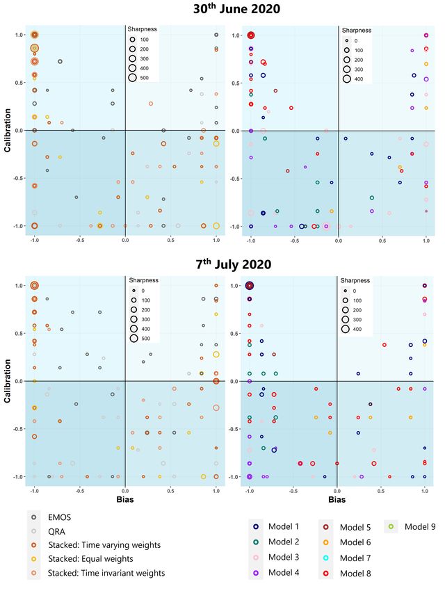
Content includes material subject to © Crown copyright (2021), Dstl. This material is licensed under the terms of the Open Government Licence
except where otherwise stated. To view this licence, visit http://www.nationalarchives.gov.uk/doc/open-government-licence/version/3 or write to
the Information Policy Team, The National Archives, Kew, London TW9 4DU, or email: psi@nationalarchives.gov.uk.

   4. interval score: SI,α (p, y) = (u − l) + α2 (l − y)1{y < l} + α2 (y − u)1{y > u} for(l, u) being a central (1 − α) ×
      100% prediction interval from p.
Quantile and interval scores can be averaged across available quantiles/intervals to provide a score for the predictive
density. The CRPS is the integral of the quantile score with respect to α. Scoring rules can be used to rank predictions
from individual models or to combine models from an ensemble, for example using stacking or regression methods.

2.2     Stacking methods
Given an ensemble of models M, stacking methods result in a posterior predictive density of the form
                                                                        K
                                                        p(ỹ | y ) =   ∑ wk pk (ỹ | y ) ,
                                                                       k=1

where pk is the (posterior) predictive density from model Mk and wk ≥ 0 weights the contribution of the kth model
to the overall prediction, with ∑k wk = 1. Giving equal weighting to each model in the stack has proved surprisingly
effective in economic forecasting [7] . Alternatively, given a score function S and out-of-sample ensemble training data
ỹ1 , . . . , ỹm , weights w = (w1 , . . . , wK )| can be chosen via

                                                                1 m
                                                         min
                                                        w ∈SK
                                                                  ∑ S(p(ỹi | y ), ỹi ) ,
                                                                m i=1
                                                                                                                                             (1)

where SK = {w w ∈ [0, 1]K : ∑k wk = 1} is the K-dimensional simplex. This approach is the essence of Bayesian model
stacking as described by Yao et al. [8] .
    Alternatively, scoring functions can be used to construct normalized weights
                                                                         f (Sk )
                                                                wk =               ,                                                         (2)
                                                                        ∑k f (Sk )
with Sk = ∑i S(pk (ỹi | y )/m being the average score for the kth model, and f being an inversely monotonic function;
with the log-score (1) and f (S) = exp(−S), Akaike Information Criterion (AIC) style weights are obtained [19] .

2.3     Regression-based methods
Ensemble model predictions can also be formed using regression methods with covariates that correspond to point
forecasts from the model ensemble. These methods are particularly suited to “low-resolution” posterior predictive
information where only posterior summaries are available and the covariates can be defined directly from, e.g., re-
ported quantiles. We consider two such regression-based methods: Ensemble Model Output Statistics [20] (EMOS)
and Quantile Regression Averaging [21] (QRA).
    EMOS defines the ensemble prediction in the form of a Gaussian distribution

                                                ŷ ∼ N(a + b1 ŷ1 + ... + bK ŷK , c + dV 2 ),                                               (3)

where ŷ1 , ..., ŷK are point forecasts from the individual models, c and d are non-negative coefficients, V = ∑k (ŷk −
ȳ)2 /(K − 1) is the ensemble variance with ȳ = ∑k ŷk /K the ensemble mean, and a and b1 , ..., bK are regression coeffi-
cients. Tuning of the coefficients is achieved by minimizing the average CRPS using out-of-sample data
                                                                       1 m
                                                          S̄c (ŷ) =     ∑ Sc (ŷ, ỹi ) .
                                                                       m i=1

For ŷ following distribution (3), Sc is available in closed form [20] . To aid interpretation, the coefficients can be
constrained to be non-negative (this version of the algorithm is known as EMOS+).
   QRA defines a predictive model for each quantile level, β , of the ensemble forecast as

                                                    ŷ(β ) = b1 ŷ1 (β ) + ... + bK ŷK (β ),                                                (4)

                                                                          3
Content includes material subject to © Crown copyright (2021), Dstl. This material is licensed under the terms of the Open Government Licence
except where otherwise stated. To view this licence, visit http://www.nationalarchives.gov.uk/doc/open-government-licence/version/3 or write to
the Information Policy Team, The National Archives, Kew, London TW9 4DU, or email: psi@nationalarchives.gov.uk.
where ŷk (β ) is the β -level quantile of the (posterior) predictive distribution for model k. We make the parsimonious
assumption that the non-negative coefficients, b1 , ...bK , are independent of the level β , and estimate them by mini-
mizing the weighted average interval score across nα central (1 − α) × 100% predictive intervals defined from the
quantiles, and m out-of-sample data points:
m
1 α
S̄I = ∑ ∑ 4 SI,α (ŷ(α), ỹi ) ,
mnα i=1 α
where the factors α/4 weight the interval scores such that at the limit of including all intervals, the score approaches
the CRPS.
3 COVID-19 pandemic forecast combinations
For the COVID-19 response, probabilistic forecasts from multiple epidemiological models were provided by members
of SPI-M at weekly intervals. Especially in the early stages of the pandemic, the model structures and parameters
were evolving to reflect increased understanding of COVID-19 epidemiology and changes in social restrictions. The
impact of evolving models is discussed in Section 5. Practical constraints on data bandwidth and rapid delivery sched-
ules resulted in individual model forecasts being reported as quantiles of the predictive distributions for the forecast
window, and minimal information was available about the individual posterior distributions. Whilst EMOS and QRA
can be directly applied using only posterior summaries, to implement stacking we estimated posterior densities as
skewed-Normal distributions fitted to each set of quantiles. Stacking weights are obtained using (2), with f taken to
be the reciprocal function [22] , that is
−1
∑m λ m−i S̄ik
wk = i=1 (5)
SK
with
S̄ik = ∑ Sq,α (ŷk (α), ỹi ) ,
α
and
K m
SK = ∑ ∑ λ m−i S̄ik−1 .
k=1 i=1
The exponential decay term (with λ = 0.9) controls the relative influence of more recent observations.
In Section 4, three choices of stacking weights are compared: (i) Reciprocal weights (5) which are invariant
with respect to future observation times t + 1, . . . ,t + m, (ii) equal weights wk = 1/K, and (iii) time-varying weights
constructed via exponential interpolation between (i) and (ii) to reduce the influence on forecasts further in the future
of the performance of individual models in the training window.
4 Comparing the performance of ensemble and individual forecasts
The performance of the different ensemble and individual forecasts from K = 9 models provided by SPI-M were
assessed over a set of 14 day forecast windows. Each model is the evolving output from teams of independent re-
searchers. Individual model predictions were provided for three different COVID-19 related quantities (see Table 1)
for different UK nations and regions (see Table 2) for the m = 20 days immediately preceding the forecast window.
Corresponding ensemble training data were obtained from government provided data streams. The individual model
predictions used were the most recently reported that had not been conditioned on data from the combination training
window. The assessment was conducted after a sufficient delay such that effects of under reporting on the obser-
vational data was negligible. However, it is unknown whether individual SPI-M models attempted to account for
potential under-reporting bias in the data used for parameter fitting.
4Content includes material subject to © Crown copyright (2021), Dstl. This material is licensed under the terms of the Open Government Licence
except where otherwise stated. To view this licence, visit http://www.nationalarchives.gov.uk/doc/open-government-licence/version/3 or write to
the Information Policy Team, The National Archives, Kew, London TW9 4DU, or email: psi@nationalarchives.gov.uk.
Value types Description
death inc line New daily deaths by date of death
hospital prev Hospital bed occupancy
icu prev Intensive care unit (ICU) occupancy
Table 1: COVID-19 value types (model outputs of interest) for which forecasts were scored.
Nations Regions
England London
Scotland East of England
Wales Midlands
Northern Ireland North East and Yorkshire
North West
South East
South West
Table 2: Nations/regions for which forecasts were scored.
We present results for the individual models and stacking, EMOS and QRA ensemble methods, as described in
Section 2. Data-driven, equal and time-varying weights were applied with model stacking, see Section 3. EMOS coef-
ficients were estimated by minimizing CRPS, with the intercept set to zero to force the combination to use the model
predictions. While this disabled some potential for bias correction, it was considered important that the combined
forecasts could be interpreted as weighted averages of the individual model predictions. QRA was parameterized via
minimization of the average of the weighted interval scores for the 0% (i.e. the quantile score for the median), 50%
and 90% prediction intervals, as described in Section 2.3. The same score was used to calculate the stacking weights
in (5). In each case, m = 20 ensemble training data points were used, and optimization was performed using a particle
swarm algorithm [23] .
Performance was measured for each model/ensemble method using the weighted average of the interval score over
the 14 day forecast window and 0%, 50% and 90% intervals. In addition, three well-established assessment metrics
were calculated; sharpness, bias and calibration [24] . Sharpness (σ ) is a measure of prediction uncertainty, and is
defined here as the average width of the 50% central prediction interval over the forecast window. Bias (β ) measures
over- or under-prediction of a predictive model as the proportion of predictions for which the reported median is
greater than the data value over the forecast window. Calibration (γ) quantifies the statistical consistency between
the predictions and data, via the proportion of predictions for which the data lies inside the 50% central predictive
interval. The bias and calibration scores were linearly transformed as β̂ = (0.5 − β )/0.5 and γ̂ = (0.5 − γ)/0.5, such
that a well-calibrated prediction with no bias or uncertainty corresponds to (β̂ , γ̂, σ ) = (0, 0, 0).
Table 3 summarizes the performance of the ensemble methods and averaged performance of the individual models
across the four forecast windows. Averaged across nations/regions, the best performing forecasts for new daily deaths
were obtained using stacking with time invariant weights; for hospital bed occupancy QRA performed best; and for
ICU occupancy, the best method was EMOS. The lowest interval scores occur when predicting new daily deaths,
reflecting the more accurate and precise individual model predictions for this output, relative to the others. The
ensemble methods also all perform similarly for this output. Importantly, every ensemble method improves upon the
average scores for the individual models. This means that with no prior knowledge about model fidelity, if a single
forecast is desired, it is better on average to use an ensemble than to select a single model.
5Content includes material subject to © Crown copyright (2021), Dstl. This material is licensed under the terms of the Open Government Licence
except where otherwise stated. To view this licence, visit http://www.nationalarchives.gov.uk/doc/open-government-licence/version/3 or write to
the Information Policy Team, The National Archives, Kew, London TW9 4DU, or email: psi@nationalarchives.gov.uk.
(a) death inc line (b) hospital prev
Model S̄I β̂ γ̂ Model S̄I β̂ γ̂
Stacked: time-invariant weights 2.16 0.66 0.49 QRA 18.0 0.80 0.78
Stacked: equal-weights 2.25 0.72 0.57 Stacked: time-invariant weights 24.5 0.81 0.68
QRA 2.28 0.65 0.51 Stacked: time-varying weights 25.4 0.84 0.77
Stacked: time-varying weights 2.43 0.76 0.45 EMOS 25.4 0.82 0.76
EMOS 2.82 0.76 0.54 Stacked: equal-weights 27.6 0.82 0.79
Models 3.03 0.77 0.61 Models 33.2 0.88 0.77
(c) icu prev
Model S̄I β̂ γ̂
EMOS 2.62 0.76 0.63
QRA 3.68 0.84 0.75
Stacked: time invariant weights 3.8 0.78 0.75
Stacked: time varying weights 3.84 0.78 0.74
Stacked: equal weights 4.07 0.79 0.77
Models 4.28 0.85 0.74
Table 3: Median interval and mean bias and calibration scores for each value type, averaged over regions/nations for
each ensemble algorithm. The mean score for the individual models is also shown. Rows are ordered by increasing
interval score in each subtable. The median was chosen for the interval score due to the presence of extreme values.
To examine the performance of the ensemble methods, and individual model predictions, in more detail, we plot
results for the nations/regions separately for different forecast windows, see Figure 1 for two examples. We plot bias
(β̂ ) against calibration (γ̂) and divide the plotting region in four quadrants; the top-right quadrant represents perhaps the
least worrying errors, as here the methods over-predict the outcomes with prediction intervals that are under-confident.
Where both observational data and model predictions were available, the metrics were evaluated for the three value
types and eleven regions/nations. Unfortunately, it is difficult to ascertain any patterns for either example. The best
forecasting model was also highly variable across nations/regions and value types (as shown for calibration and bias
in Figure 2), and was often an individual model.
The variability in performance was particularly stark for QRA and EMOS, which were found in some cases to
vastly outperform the individual and stacked forecasts, and in others to substantially under-perform (as shown in
Figure 3). The former case generally occurred when all the individual model training predictions were highly biased
(for example, for occupied ICU beds in the South West for the 23rd June forecast). In these cases, the non-convexity of
the QRA and EMOS coefficients led to forecasts that were able to correct for this bias. The problem of bias correction
is, of course, the case for which these methods were originally proposed in weather forecasting. Whether this behaviour
is desirable depends upon whether the data is believed to be accurate, or itself subject to large systematic biases, such as
under-reporting, that is not accounted for within the model predictions. The latter case of under-performance occurred
in the presence of large discontinuities between the individual model training predictions and forecasts, corresponding
to changes in model structure or parameters. This disruption to the learnt relationships between individual model
predictions, and to the data (as captured by the regression models), led to increased forecast bias (an example of this
is shown in Figure 4).
6Content includes material subject to © Crown copyright (2021), Dstl. This material is licensed under the terms of the Open Government Licence
except where otherwise stated. To view this licence, visit http://www.nationalarchives.gov.uk/doc/open-government-licence/version/3 or write to
the Information Policy Team, The National Archives, Kew, London TW9 4DU, or email: psi@nationalarchives.gov.uk.
Figure 1: Sharpness, bias and calibration scores for the (left) individual and (right) ensemble forecasts, for all regions
and value types delivered on (top) 30th June and (bottom) 7th July, 2020. Note that multiple points are hidden when
they coincide. The shading of the quadrants (from darker to lighter) implies a preference for over-prediction rather
than under-prediction, and for prediction intervals that contain too many data points, rather than too few.
7Content includes material subject to © Crown copyright (2021), Dstl. This material is licensed under the terms of the Open Government Licence
except where otherwise stated. To view this licence, visit http://www.nationalarchives.gov.uk/doc/open-government-licence/version/3 or write to
the Information Policy Team, The National Archives, Kew, London TW9 4DU, or email: psi@nationalarchives.gov.uk.
Figure 2: The best performing individual model or ensemble method for each region/nation and value type (for fore-
casts delivered on the 23rd and 30th June, and 7th and 14th July 2020), evaluated using the absolute distance from the
origin on the calibration-bias plots. Ties were broken using the sharpness score. For each date, only the overall best
performing model / ensemble is displayed, but for clarity the results are separated into (left) individual models and
(right) combinations. Region/nation and value type pairs for which there was less than two individual models with
both training and forecast data available were excluded from the analysis.
8Content includes material subject to © Crown copyright (2021), Dstl. This material is licensed under the terms of the Open Government Licence
except where otherwise stated. To view this licence, visit http://www.nationalarchives.gov.uk/doc/open-government-licence/version/3 or write to
the Information Policy Team, The National Archives, Kew, London TW9 4DU, or email: psi@nationalarchives.gov.uk.
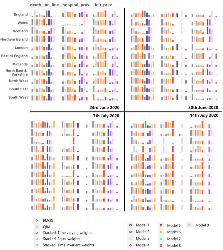
Figure 3: Performance of individual models and ensemble methods for each region/nation and value type (for fore-
casts delivered on the 23rd and 30th June, and 7th and 14th July 2020). The height of each bar is calculated as the
reciprocal of the weighted average interval score, so that higher bars correspond to better performance. Gaps in the
results correspond to region/nation and value type pairs for a which a model did not provide forecasts. No combined
predictions were produced for Scotland hospital prev on the 7th July as forecasts were only provided from a single
model.
9Content includes material subject to © Crown copyright (2021), Dstl. This material is licensed under the terms of the Open Government Licence
except where otherwise stated. To view this licence, visit http://www.nationalarchives.gov.uk/doc/open-government-licence/version/3 or write to
the Information Policy Team, The National Archives, Kew, London TW9 4DU, or email: psi@nationalarchives.gov.uk.
Figure 4: QRA forecast for hospital bed occupancy in the North West region. A large discontinuity between the
current and past forecasts (black line) of the individual model corresponding to the covariate with the largest regression
coefficient can lead to increased bias for the QRA algorithm. The median, 50% and 90% QRA prediction intervals are
shown in blue, while the data is shown in red.
In comparison, the relative performance of the stacking methods was more stable across different regions/nations
and value types (see Figure 3), which likely reflects the conservative nature of the simplex weights in comparison to
the optimized regression coefficients. In terms of sharpness, the stacked forecasts were always outperformed by the
tight predictions of some of the individual models, and by the EMOS method.
It is worth noting the delay in the response of the combination methods to changes in individual model perfor-
mance. For example, the predictions from model eight for hospital bed occupancy in the Midlands improved consider-
ably to become the top performing model on 7th July. The weight assigned to this model, for example in the stacking
with time-invariant weights algorithm, increased from 15% on 7th July to 48% on the 14th July, but only became
the highest weighted model (87%) for the forecast window beginning on 21st July. This behaviour arises from the
requirement for sufficient training data from the improved model to become available in order to detect the change in
performance.
5 Discussion
Scoring rules are a natural way of constructing weights for forecast combination. In comparison to Bayesian model
averaging, weights obtained from scoring rules are directly tailored to approximate a predictive distribution, and reduce
sensitivity to the choice of prior distribution. Crucially use of scoring rules avoids the pitfall associated with model
averaging of convergence to a predictive density from a single model, even when the ensemble of models does not
include the true data generator. Guidance is available in the literature for which situations different averaging and
ensemble methods are appropriate Höge et al. [25] .
In this study, several methods (stacking, EMOS and QRA) to combine epidemiological forecasts have been inves-
10Content includes material subject to © Crown copyright (2021), Dstl. This material is licensed under the terms of the Open Government Licence
except where otherwise stated. To view this licence, visit http://www.nationalarchives.gov.uk/doc/open-government-licence/version/3 or write to
the Information Policy Team, The National Archives, Kew, London TW9 4DU, or email: psi@nationalarchives.gov.uk.
tigated within the context of delivery of scientific advice to decision makers during a pandemic. Their performance
was evaluated using the well-established sharpness, bias and calibration metrics as well as the interval score. When
averaged over nations/regions, the best performing forecasts according to both the metrics and interval score, orig-
inated from the time-invariant weights stacking method for new daily deaths, EMOS for ICU occupancy, QRA for
hospital bed occupancy. However, the performance metrics for each model and ensemble method were found to vary
considerably over the different regions and value type combinations. Whilst some individual models were observed to
perform consistently well for particular region and value type combinations, the extent to which the best performing
models remain stable over time requires further investigation using additional forecasting data.
The rapid evolution of the models (through changes in both parameterization and structure) during the COVID-19
outbreak has led to substantial changes in each model’s predictive performance over time. This represents a signifi-
cant challenge for ensemble methods that essentially use a model’s past performance to predict its future utility, and
has resulted in cases where the ensemble forecasts do not represent an improvement to the individual model forecasts.
For the stacking approaches, this challenge could be overcome by either (a) additionally providing quantile predictions
from the latest version of the models for (but not fit to) data points within a training window, or (b) sampled trajectories
from the posterior predictive distribution for the latest model at data points that have been used for parameter estima-
tion. Option (a) would allow direct application of the current algorithms to the latest models but may be complicated
by addition of model structure due to, for example, changes in control measures, whilst (b) would enable application
of full Bayesian stacking approaches using, for example, leave-one-out cross validation [8] . However, it is important
to consider the practical constraints on the resolution of information available during the rapid delivery of scientific
advice during a pandemic. With no additional information, it is possible to make the following simple modification to
the regression approaches to reduce the prediction bias associated with changes to the model structure or parameters.
Analysis of the individual model forecasts revealed large discrepancies between the past and present forecasts for
an individual model could lead to increased bias, particularly for the QRA and EMOS combined forecasts. Overlap-
ping of past and present forecasts allows this discrepancy to be characterized, and its impact reduced by translating
the individual model predictions (covariates) at time t (ỹk (α)) in the regression models) match the training predictions
for the start of the forecast window, t0 . For cases where the discrepancy is large (e.g. Figure 4), the reduction in bias
of this shifted QRA (SQRA) over QRA is striking, see Figure 5).
11Content includes material subject to © Crown copyright (2021), Dstl. This material is licensed under the terms of the Open Government Licence
except where otherwise stated. To view this licence, visit http://www.nationalarchives.gov.uk/doc/open-government-licence/version/3 or write to
the Information Policy Team, The National Archives, Kew, London TW9 4DU, or email: psi@nationalarchives.gov.uk.
Figure 5: QRA (blue) and Shifted QRA (SQRA; green) forecasts for hospital bed occupancy in the North West region
for a forecast window beginning on 14 May. SQRA corrects for the discontinuity between past and current forecasts
for the individual model (black line) that corresponds to the covariate with the largest coefficient. Data is shown in
red.
S̄I β̂ γ̂
death inc line 1.86 0.45 0.46
hospital prev 24.0 0.86 0.72
icu prev 2.23 0.66 0.63
Table 4: Median interval, and mean bias and calibration scores for SQRA for each value type, over the four forecast
windows.
Table 4 shows the average interval scores for the SQRA algorithm over the four forecast windows. For new daily
deaths and ICU occupancy, the SQRA algorithm achieves better median scores than the other methods considered.
These promising results motivate future research into ensemble methods that are robust to the practical limitations
imposed by the pandemic response context.
Acknowledgments
The research in this paper was undertaken as part of the CrystalCast project, which is developing and implementing
methodology to enhance, exploit and visualize scientific models in decision-making processes.
This work has greatly benefited from parallel research led by Sebastian Funk (LSHTM), and was conducted within
a wider effort to improve the policy response to COVID-19. The authors would like to thank the SPI-M modelling
groups for the data used in this paper. We would also like to thank Tom Finnie at PHE and the SPI-M secretariat for
their helpful discussions.
12Content includes material subject to © Crown copyright (2021), Dstl. This material is licensed under the terms of the Open Government Licence
except where otherwise stated. To view this licence, visit http://www.nationalarchives.gov.uk/doc/open-government-licence/version/3 or write to
the Information Policy Team, The National Archives, Kew, London TW9 4DU, or email: psi@nationalarchives.gov.uk.
(c) Crown copyright (2020), Dstl. This material is licensed under the terms of the Open Government License
except where otherwise stated. To view this license, visit http://www.nationalarchives.gov.uk/doc/open-government-
licence/version/3 or write to the Information Policy Team, The National Archives, Kew, London TW9 4DU, or email:
psi@nationalarchives.gsi.gov.uk
References
[1] M. A. Semenov and P. Stratonovitch. Use of multi-model ensembles from global climate models for assessment
of climate change impacts. Climate research, 41:1–14, 2010.
[2] A. E. Raftery, D. Madigan, and J. A. Hoeting. Bayesian model averaging for linear regression models. Journal
of the American Statistical Association, 92:179–191, 1997.
[3] D. Madigan, A. E. Raftery, C. Volinsky, and J. Hoeting. Bayesian model averaging. In Proceedings of the AAAI
Workshop on Integrating Multiple Learned Models, Portland, OR, pages 77–83, 1996.
[4] J. A. Hoeting, D. Madigan, A. E. Raftery, and C. T. Volinsky. Bayesian model averaging: a tutorial. Statistical
Science, pages 382–401, 1999.
[5] K. F. Wallis. Combining density and interval forecasts: a modest proposal. Oxford Bulletin of Economics and
Statistics, 67:983–994, 2005.
[6] T. Gneiting, A. E. Raftery, A. H. Westveld III, and T. Goldman. Calibrated probabilistic forecasting using
ensemble model output statistics and minimum CRPS estimation. Monthly Weather Review, 133:1098–1118,
2005.
[7] C. McDonald and L. A. Thorsrud. Evaluating density forecasts: model combination strategies versus the RBNZ.
Technical Report DP2011/03, Reserve Bank of New Zealand, 2011.
[8] Y. Yao, A. Vehtari, D. Simpson, and A. Gelman. Using stacking to average Bayesian predictive distributions
(with discussion). Bayesian Analysis, 13:917–1007, 2018.
[9] T. P. Minka. Bayesian model averaging is not model combination. Available electronically at http://www. stat.
cmu. edu/minka/papers/bma. html, pages 1–2, 2000.
[10] K. Monteith, J. L. Carroll, K. Seppi, and T. Martinez. Turning Bayesian model averaging into Bayesian model
combination. In The 2011 International Joint Conference on Neural Networks, pages 2657–2663. IEEE, 2011.
[11] M. C. Kennedy and A. O’Hagan. Bayesian calibration of computer models (with discussion). Journal of the
Royal Statistical Society B, 63:425–464, 2001.
[12] Scientific Advisory Group for Emergencies. SPI-M-O: COVID-19 short-term forecasting: Academic summary
positions, 2 April 2020. GOV.UK Coronavirus (COVID-19) Rules, guidance and support, 2020.
[13] Scientific Advisory Group for Emergencies. Combining forecasts (s0123). GOV.UK Coronavirus (COVID-19)
Rules, guidance and support, 2020.
[14] Scientific Advisory Group for Emergencies. Combining model forecast intervals (s0124). GOV.UK Coronavirus
(COVID-19) Rules, guidance and support, 2020.
[15] T. Maishman, S. Schaap, D. S. Silk, S. J. Nevitt, D. C. Woods, and V. E. Bowman. Statistical methods
used to combine the effective reproduction number, R(t), and other related measures of COVID-19 in the UK.
arXiv:2103.01742, 2021.
[16] S. Funk et al. Short-term forecasts to inform the response to the covid-19 epidemic in the uk. Submitted to
Statistical Methods in Medical Research, 2021.
13Content includes material subject to © Crown copyright (2021), Dstl. This material is licensed under the terms of the Open Government Licence
except where otherwise stated. To view this licence, visit http://www.nationalarchives.gov.uk/doc/open-government-licence/version/3 or write to
the Information Policy Team, The National Archives, Kew, London TW9 4DU, or email: psi@nationalarchives.gov.uk.
[17] T. Gneiting and A. E. Raftery. Strictly proper scoring rules, prediction and estimation. Journal of the American
Statistical Association, 102:359–378, 2007.
[18] T. Gneiting and R. Ranjan. Comparing density forecasts using threshold- and quantile-weighted scoring rules.
Journal of Business and Economic Statistics, 29:411–422, 2011.
[19] K. P. Burnham and D. R. Anderson. Model Selection and Multimodel Inference. Springer, New York, 2nd edition,
2002.
[20] Tilmann Gneiting, Adrian E Raftery, Anton H Westveld III, and Tom Goldman. Calibrated probabilistic fore-
casting using ensemble model output statistics and minimum crps estimation. Monthly Weather Review, 133(5):
1098–1118, 2005.
[21] Jakub Nowotarski and Rafał Weron. Computing electricity spot price prediction intervals using quantile regres-
sion and forecast averaging. Computational Statistics, 30(3):791–803, 2015.
[22] Chris McDonald, Leif Anders Thorsrud, et al. Evaluating density forecasts: model combination strategies versus
the rbnz. Technical report, Reserve Bank of New Zealand, 2011.
[23] James Kennedy and Russell Eberhart. Particle swarm optimization. In Proceedings of ICNN’95-International
Conference on Neural Networks, volume 4, pages 1942–1948. IEEE, 1995.
[24] Tilmann Gneiting, Fadoua Balabdaoui, and Adrian E Raftery. Probabilistic forecasts, calibration and sharpness.
Journal of the Royal Statistical Society: Series B (Statistical Methodology), 69(2):243–268, 2007.
[25] M. Höge, A. Guthke, and W. Nowak. The hydrologist’s guide to Bayesian model selection, averaging and
combination. Journal of Hydrology, 572:96–107, 2019.
14You can also read