Ultra-High-Energy Neutrino Detection Antenna Simulations June 2021 By: Nicholas Garcia Advisor: Dean Arakaki Electrical Engineering Department ...

Ultra-High-Energy
 Neutrino Detection Antenna
 Simulations

 June 2021

 By: Nicholas Garcia
 Advisor: Dean Arakaki

 Electrical Engineering Department
California Polytechnic State University

 1

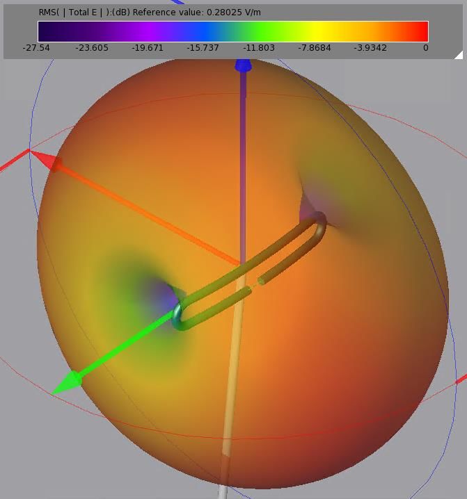
Table of Contents
 List of Tables ............................................................................................................................................. 2
 List of Figures ............................................................................................................................................ 3
Acknowledgements ....................................................................................................................................... 4
Abstract ......................................................................................................................................................... 5
Chapter 1. Introduction and Background ..................................................................................................... 6
Chapter 2. Antenna Design ........................................................................................................................... 9
Chapter 3. System Design Tradeoffs ........................................................................................................... 15
Chapter 4. Analysis and Simulation Results ................................................................................................ 16
Chapter 5. Suggestions for Improvement ................................................................................................... 36
References .................................................................................................................................................. 38
Appendix A. Senior Project Analysis ........................................................................................................... 39

List of Tables
Table 1 .......................................................................................................................................................... 8
Table 2 ........................................................................................................................................................ 10
Table 3 ........................................................................................................................................................ 10
Table 4 ........................................................................................................................................................ 12
Table 5 ....................................................................................................................................................... 13
Table 6 ....................................................................................................................................................... 21
Table 7 ....................................................................................................................................................... 23
Table 8 ....................................................................................................................................................... 27
Table 9 ....................................................................................................................................................... 30
Table 10 ..................................................................................................................................................... 33

 2

List of Figures
Figure 1. ........................................................................................................................................................ 6
Figure 2 ......................................................................................................................................................... 7
Figure 3. ........................................................................................................................................................ 7
Figure 4. ........................................................................................................................................................ 8
Figure 5. ........................................................................................................................................................ 9
Figure 6. ...................................................................................................................................................... 10
Figure 7 ....................................................................................................................................................... 11
Figure 8. ...................................................................................................................................................... 12
Figure 9. ...................................................................................................................................................... 14
Figure 10. .................................................................................................................................................... 16
Figure 11. .................................................................................................................................................... 17
Figure 12 ..................................................................................................................................................... 18
Figure 13. .................................................................................................................................................... 19
Figure 14. .................................................................................................................................................... 20
Figure 15. .................................................................................................................................................... 22
Figure 16. .................................................................................................................................................... 23
Figure 17 ..................................................................................................................................................... 24
Figure 18. .................................................................................................................................................... 24
Figure 19. .................................................................................................................................................... 25
Figure 20. .................................................................................................................................................... 25
Figure 21. .................................................................................................................................................... 26
Figure 22 ..................................................................................................................................................... 26
Figure 23. .................................................................................................................................................... 28
Figure 24. .................................................................................................................................................... 29
Figure 25. .................................................................................................................................................... 30
Figure 26. .................................................................................................................................................... 31
Figure 27 ..................................................................................................................................................... 32
Figure 28. .................................................................................................................................................... 33
Figure 29. .................................................................................................................................................... 34
Figure 30. .................................................................................................................................................... 35
Figure 31. .................................................................................................................................................... 37

 3

Acknowledgements

Thank you to everyone who has been involved with this project for their provided insight and assistance:

Kerr Allan, Jissell Jose, John Kimura, Diego Masini, Joseph Nuccio, Garrett Knoller, Dan Southall, and

 Bryan Hendricks

Special thanks to Dr. Dean Arakaki and Dr. Stephanie Wissel for their guidance and growing my passion

 for RF engineering.

 4

Abstract
Neutrinos allow researchers to investigate high-energy galactic phenomena, such as supernovae and black holes.

Neutrinos interact with their surroundings via the weak nuclear force and therefore, travel unattenuated through

space and are not deflected by electromagnetic fields. However, they do rarely interact with other particles. When

neutrinos interact with nucleons (protons or neutrons) in a dielectric medium (i.e.: ice sheets), they are detectable

through a cone of coherent electromagnetic radiation (Askaryan Radiation) created by the particle shower generated

from the neutrino interaction [1]. The Radio Neutrino Observatory in Greenland (RNO-G) detects UHE neutrinos

greater than 100 PeV (1015 eV) in energy. For reference, that level of energy is enough to lift an apple 5cm or drive

the 100 PeV neutrino, which is nearly massless, near the speed of light [2]. Antennas operating in the bandwidth of

200MHz to 1000MHz detect impulse responses from neutrino-ice Askaryan radiation. This paper addresses the

suitability of normal mode helical antenna (NMHA) and folded dipole antenna performance in detecting neutrino-

induced radiation. The NMHA was selected over an axial mode helical antenna due to its omnidirectional radiation

pattern and borehole (RNO-G antenna deployment) constraints.

 5

Chapter 1. Introduction and Background

RNO-G’s main objective is to detect and characterize UHE neutrino events. Such events are recorded by 35 stations

onsite in Greenland [3]. Each station consists of 3 boreholes 10-inches in diameter and 100m deep into the ice;

displayed in Figure 1 [4].

 Figure 1. Aerial Schematic View of RNO-G’s Layout (left) and Borehole Antenna Configuration (right)

RNO-G is based on the previous phased array antenna station located at the South Pole: Askaryan Radio Array

(ARA) [5]. The ARA antennas contain ferrites which increase deployment weight and simulation complexity [6].

To eliminate the ferrites, a tri-slot antenna feed was characterized using dipole antennas [7]. However, the design

did not meet broadband requirements; a matching network was implemented to increase bandwidth [8]. A

bandwidth of 425-750MHz was achieved. The objective is to investigate the NMHA and folded dipole |S11| vs.

frequency, S11 vs. frequency on a Smith Chart, and horizontal vs. vertical polarization using the antenna simulation

software XFdtd. The NMHA and folded dipole (see Figure 2) represent potential replacements for the tri-slot.

 6

a. Helical Antenna Dimensions b. Folded Dipole Dimensions

 Figure 2. Helical Antenna Dimensions (2a) and Folded Dipole Dimensions (2b) [9]

 Figure 3. Visualization of Horizontal (H) and Vertical (V) Polarization [10]

To ensure the integrity of the NMHA simulation model it is compared to the NMHA found in [11]. Figure 4 shows

the difference between normal and axial mode helical antennas [12].

 7

a. Normal Mode b. Axial Mode

 Figure 4. Normal Mode and Axial Mode Helical Antenna Radiation Patterns

The NMHA is advantageous for RNO-G due to the antenna’s orientation in boreholes. The normal mode detects

signals on the broadside (red region of Figure 4a) of the antenna, whereas the axial mode’s main lobe occurs at θ =

0⁰.

The folded dipole can be considered a single λ/2 dipole because the two λ/2 dipole currents are sufficiently close

together in space [13]. Input and output characteristics are shown in Table 1.

 Table 1: Inputs, Outputs, and Functionality

 Inputs Electromagnetic Askaryan Radiation

 - Horizontally polarized signal
 - Frequency Range: 200MHz to 1000MHz
 Outputs Measured Radiation Signal

 Functionality Detects horizontally polarized neutrino Askaryan
 radiation to determine UHE neutrino energy level
 and direction of origin.

 8

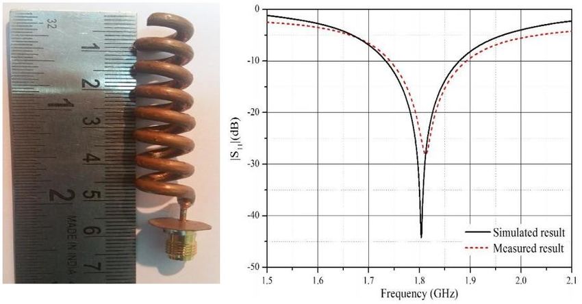
Chapter 2. Antenna Design

Section 2.1: NMHA Design

IIT Bombay’s normal mode helical antenna (NMHA) has an |S11| vs. frequency response from [11] is

shown below in Figure 5. Simulations are outside the 200MHz to 1000MHz bandwidth but are used as a

baseline for a comparing verified results with the XFdtd model’s |S11| vs. frequency.

 Figure 5. IIT Bombay NMHA and |S11| (dB) vs. frequency (GHz) response.

 9

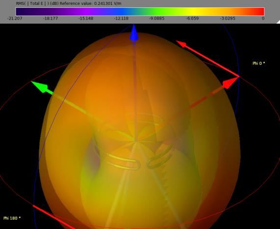
Table 2 lists the dimensions of the IIT Bombay antenna and the NMHA recreated in XFdtd [11].

 Table 2: Helical Antenna Dimensions of XFdtd Simulation

 Resonant Frequency (GHz) 1.8

 Wavelength (mm) 166

 Spacing (0.027λ) (mm) 4.5

 Diameter of Helix (0.033λ) 5.5

 Number of Turns (N) 7

 Pitch angle (α in degrees) 14.6

 Diameter of Ground Plane (λ/28) (mm) 5.9

 Wire thickness (λ/100) (mm) 1.6 (16 gauge)

 Radius of Hole (b) in Ground Plane (0.038 λ) (mm) 3.18

 (Size determined on next page)

 Material Copper

The XFdtd NMHA was modeled with a hole in the ground plane to simulate the outer diameter of a 50Ω

coaxial cable feed. The authors of [11] specified inner diameter, 2a, of the coaxial cable as 1.2mm.

Figure 6 defines the coaxial cable and its parameters.

 Table 3 Coaxial Cable Parameters
 2a (mm) 1.2

 εr 2

 µr 1

 Z0 (Ω) 50

 Figure 6. Coaxial Cable Model and Tabulated Parameters.

 10

The outer radius b of the ground plane was calculated using equation 1 [14]:

 0 = 60√ ln ( )
 (1)

Since µr is 1, the equation in terms of b is:

 0 √ (2)
 = 60

The NMHA CAD model is constructed in XFdtd; see Figure 7. The feed structure includes a hole in the

ground plane to approximate the 50Ω coaxial cable feed. The XFdtd line source is shown in green and

models a 50Ω voltage source.

 6a. Portrait View 6a. Top-Down View

 Figure 7. IIT Bombay NMHA in XFdtd Portrait View (6a) and Top-Down View (6b)

 11

Section 2.2: Folded Dipole Design

The dimensions of a single, folded dipole are d = 40 mm by L = 240 mm [15]. The L dimension of the

folded dipole was calculated assuming a 600MHz center frequency, which yields an uncompensated half-

wave dipole length of 0.25m. Wire radius compensation is accomplished through the following table 5 [9].

 Table 4 Compensation of Folded Dipole Length Due to Wire Radius

 This dipole falls into the “thin” class, resulting in a final length of 237.5mm. The design is 240mm

in length following XFdtd design optimization; see Figure 8. The extra 2.5mm length is due to the nonzero

wire radius to form the folded dipole.

 Figure 8. Folded Dipole Geometry

 12

The folded dipole was designed to operate at 600MHz. The midband frequency was reduced after

dimension optimization in XFdtd; see Table 5.

 Table 5 Folded Dipole Dimensions at Midband 512.5MHz

 Dimension Value

 Midband Frequency (MHz) 512.5

 Wavelength (m) 0.585

 L (0.41λ) (mm) 240

 d (0.07λ) (mm) 40

 Wire Radius a (0.01λ) (mm) 5.0

 13

Section 2.3: Bowed Folded Dipole Design

The motivation for bending the folded dipole (see Figure 9) is to create a folded dipole array of two or three

elements inside the borehole. The bowed folded dipole has the same dimensions listed in Table 5. However,

the antenna length was bowed to observe the effects on |S11| vs. frequency, radiation pattern, and midband

frequency.

 Figure 9. Bowed Folded Dipole Geometry

 14

Chapter 3. System Design Tradeoffs

A primary design tradeoff is the number of antennas in the bowed folded dipole array. A more uniform

radiation pattern can be achieved by increasing the number of antennas in the plane. Increasing the

number of elements in the array and remaining in the 200MHz to 1000MHz bandwidth is limited due to

the borehole radius. The borehole is limited by the size and cost of drills available.

 15

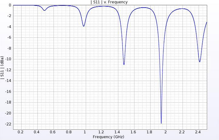
Chapter 4. Analysis and Simulation Results

Section 4.1: NMHA Results

Comparing XFdtd Model to IIT Bombay NMHA

Figure 10 displays the XFdtd NMHA model’s |S11| vs frequency response.

 Figure 10. XFdtd NMHA |S11| vs. frequency response.

 The |S11| vs. frequency responses in Figures 5 and 10 have nulls at a 1.8GHz and 1.9GHz,

 respectively. The two simulations differ due to the authors of [11] including a full model of the feed

 in their simulations. The XFdtd NMHA approximates the midband frequency of [11] within 6%.

 16

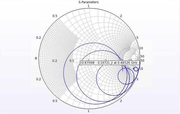
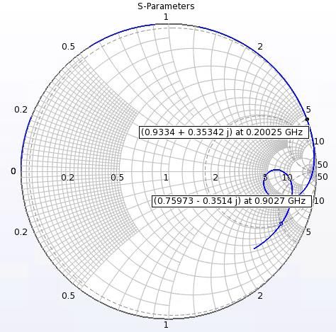
Figure 11 displays the XFdtd Smith Chart of the point which corresponds to the midband frequency.

A series inductor can be used to match the feed to a 50 coaxial cable at the midband frequency to

increase |S11| bandwidth.

 Figure 11. XFdtd NMHA Smith Chart Response

 17

Investigation of a Tapped Feed

A tapped feed (see Figure 12) was used to determine its effects on |S11| vs. frequency and S11 vs.

frequency on Smith Chart. The tapped feed is situated 1 helical turn above the original feed location

shown in Figure 6.

 Figure 12. Tapped Feed NMHA

 18

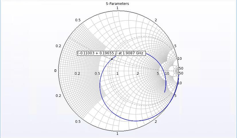
The tapped feed reduces |S11| at the midband frequency; see Figure 13a. Figure 13b shows tapping the

feed causes the response to be less circular than shown in Figure 11.

a. Tapped Feed NMHA |S11| vs. Frequency b. Tapped Feed NMHA S11 vs Frequency on Smith Chart

 Figure 13. Tapped Feed NMHA |S11| vs. Frequency (13a) and S11 vs Frequency on Smith Chart (13b)

Tapping the feed is not good for the overall design because it reduces null depth in |S11| vs. frequency and

does not cause tighter impedance clustering on the Smith Chart.

 19

Investigation of Increasing Hole Radius in NMHA Ground Plane

An investigation of ground hole size and its effects on |S11| vs. frequency is shown in Figure 14. The

NMHA otherwise has the same dimensions listed in Table 2.

 a. NMHA with 0.1mm Hole Radius in b. NMHA with 0.2mm Hole Radius in
 Ground Plane Ground Plane

 c. NMHA with 0.3mm Hole Radius in
 Ground Plane
 Figure 14. NMHA |S11| vs. Frequency for Different Sized Hole Radius in Ground Plane

As the size of the hole in the ground plane increases, null depth decreases and midband frequency

minimally decreases. The results are shown in Table 6.

 20

Table 6 Results of Increasing Hole Radius in NMHA Ground Plane

 Radius of Hole (mm) Null Depth (dB) Midband Frequency (GHz)

 0.1 -15.12 1.9098

 0.2 -14.75 1.9098

 0.3 -13.27 1.9004

A smaller hole radius in NMHA ground plane is beneficial. Note that as hole radius decreases, so too does

the characteristic impedance of the approximated coaxial cable feed line. 50Ω coaxial cables are widely

available so it is suggested to keep the hole radius in the ground plane the same as in Table 2.

 21

Decreasing NMHA Midband Frequency

To lower the midband frequency the XFdtd NMHA height was increased; results shown in Figure 15.

Recall the original number of turns was 8 and antenna height was 31.5mm.

 a. 11 turns (49.5 mm height) b. 15 turns (67.5 mm height)

 c. 20 turns (90 mm height) d. 50 turns (225 mm height)

 Figure 15. XFdtd NMHA |S11| vs. Frequency Response with Increased Antenna Heights

 22

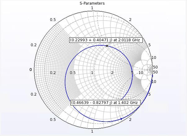
The results are tabulated in Table 7 and shows increasing NMHA height and decreases both the midband

frequency and null depth.

 Table 7 Midband Frequency and Notch Depth Related to NMHA turns/height

 Turns Height (mm) f0 (GHz) Notch Depth (dB)

 11 49.5 1.65 -13

 15 67.5 1.35 -7

 20 90.0 1.00 -5

 50 225.0 0.50 -1

The 50-turn NMHA Smith Chart shown in Figure 16 displays impedance clustering. Including a matching

network will shift the midband frequency to the Smith Chart origin to decrease null depth and increase

bandwidth.

 Figure 16. 50-turn NMHA Smith Chart

 23

The 50-turn NMHA radiation pattern is omnidirectional, as desired; shown in Figure 17. The polarization

of the antenna is determined by extracting the radiation pattern data from XFdtd and importing it into

MATLAB.

 Figure 17. Total Radiation Pattern of NMHA

The NMHA is dominantly vertically polarized. Figure 18 shows |Ephi/Etheta| (horizontal to vertical

polarization) sweeping 360⁰ of φ with a fixed θ of 90⁰. The mean |Ephi/Etheta| is approximately 0.062,

indicating the NMHA is dominantly vertically polarized.

 Figure 18. |Ephi/Etheta| vs. Angle Phi, Fixed θ = 90⁰

 24

Effects of Decreasing Pitch Angle and Increasing Helix Radius

A simulation to explore how decreasing antenna pitch angle affects midband frequency and polarization

was done. The |S11| vs. frequency characteristics are included to determine the changes in midband

frequency. Figure 19 shows decreasing pitch angle and decreases midband frequency. Figure 20 shows

the ratio of horizontal to vertical polarization decreases with a decreasing pitch angle. The decreased

midband frequency is beneficial to the final design, but the ratio of horizontal to vertical polarization

decreased.

 a. Helix Rad = 2.25mm (α = 10.2⁰) b. Helix Rad = 2.25mm (α = 12.3⁰)
 Figure 19. |S11| vs. Frequency for Fixed Radius of 2.25mm and Differing Pitch Angles

 a. Helix Rad = 2.25mm (α = 10.2⁰) b. Helix Rad = 2.25mm (α = 12.3⁰)
 Figure 20. Horizontal to Vertical Polarization Ratios for Theta = 90⁰

 25

Figure 21 shows a 3.5mm helix radius and the pitch angles of 10.2⁰ and 12.3⁰ were inspected again. The

increase in radius increases the midband frequency for both pitch angles.

 a. Helix Rad = 3.5mm (α = 10.2⁰) b. Helix Rad = 3.5mm (α = 12.3⁰)
 Figure 21. |S11| vs. Frequency for Fixed Radius of 3.5mm and Differing Pitch Angles

Comparing Figures 20 and 22 indicates the ratio of horizontal to vertical polarization increases as helix

radius increases. The effect is expected because the dimensions of the antenna are widening causing more

horizontal electric potential across the helical coils. Although there is an increase in horizontal

polarization, it is minimal. For instance, a ratio of 1 indicates equal horizontal to vertical polarization and

the maximum ratio in Figure 22b is 0.00335.

 a. Helix Rad = 3.5mm (α = 10.2⁰) b. Helix Rad = 3.5 mm (α = 12.3⁰)
 Figure 22. Horizontal to Vertical Polarization Ratios for Theta = 90⁰

 26

The NMHA is dominantly vertically polarized and is a potential candidate for a vertically polarized

antenna if a matching network is implemented. Table 8 shows the results of the NMHA and its

requirements.

 Table 8 NMHA Results Compared with Requirement

 Characteristic Result Requirement

 Midband Frequency 500MHz 500MHz (approximately)

 Polarization Vertical Horizontal

 Potential Bandwidth Match 300MHz to 1000MHz 200MHz to 1000MHz

 Deployable in Borehole Yes Yes

 27

Section 4.2: Folded Dipole Results

The folded dipole is designed for a midband frequency of 600MHz. However, after optimization in XFdtd

the midband frequency is 512.5MHz. Figure 23 shows the folded dipole |S11| vs. frequency response and

its Smith Chart.

 a. |S11| vs. Frequency b. S11 vs. Frequency on Smith Chart
 Figure 23. |S11| vs. Frequency (21a) and S11 vs. Frequency on Smith Chart (21b)

Figure 23b shows an impedance cluster near the midband frequency. If matched, the overall system will

decrease the null and frequencies near the midband. A matching network consisting of a shunt capacitor

(shift impedance cluster to r = 1 circle on Smith Chart) and a series inductor (shift impedance cluster to

origin of smith chart along r = 1 circle) should accomplish the match.

 28

Figure 24 shows the folded dipole’s radiation pattern at a frequency of 500MHz.

 Figure 24. The Folded Dipole’s Omnidirectional Radiation Pattern

Similar to a λ/2 dipole, the folded dipole has an omnidirectional radiation pattern. The two “arms” of the

folded dipole carry identical, half-wave sinusoidal current distributions [9]. The currents are close

together and the antenna is treated as a single λ/2 dipole. Hence, the directivity of the folded dipole is

identical to that of the half-wave dipole.

 29

Figure 25 displays the mean of the ratio of horizontal to vertical polarization swept 360⁰ in φ (in 5⁰

increments) for every 5⁰ increment of θ from θ = 0⁰ to θ = 180⁰. The folded dipole is dominantly

horizontally polarized having a minimum mean horizontal to vertical polarization ratio of 18.6 to 1, which

corresponds to a minimum 94.9% horizontal polarization.

 Figure 25. Mean Horizontal to Vertical Polarization vs. θ (⁰) ~ 5⁰ resolution in φ and θ.
 Minimum Eh/Ev Value: 18.6

The folded dipole is a good candidate for a horizontally polarized neutrino detection antenna due to its

horizontal polarization, potential to be matched to a 50Ω coaxial cable, midband frequency, and size.

Table 9 shows the results of the folded dipole and its requirements.

 Table 9 Folded Dipole Results Compared with Requirement

 Characteristic Result Requirement

 Midband Frequency 512.5MHz 500MHz (approximately)

 Polarization Horizontal Horizontal

 Potential Bandwidth Match 300MHz to 1000MHz 200MHz to 1000MHz

 Deployable in Borehole Yes Yes

 30

Section 4.3: Bowed Folded Dipole Results

The bowed folded dipole has the same specifications as the folded dipole, but it is bowed to resemble and

arc length. Comparing Figures 23 and 26 shows |S11| vs. frequency maintains a similar response over

200MHz to 1000MHz and null depth increases as bend angle  increases. Therefore, changes made to the

folded dipole should also apply to the bowed folded dipole [15].

 a. |S11| vs. Frequency:  = 10⁰, 20⁰, 30⁰, and 40⁰ b. S11 vs. Frequency on Smith Chart
 Figure 26. Bent Dipole |S11| vs. Frequency: bow angle  = 10⁰, 20⁰, 30⁰, and 40⁰ (6a)
 and S11 vs. Frequency on Smith Chart: bow angle  = 40⁰ (6b)

Figure 26b shows a matching network from load to feed consisting of a shunt capacitor and a series

inductor should be implemented to increase the bandwidth and notch depth of the bent folded dipole.

 31

Figure 27 shows the bowed folded dipole’s omnidirectional radiation pattern and the effect of increasing

bend angle . As the bend angle increases the null depth decreases. This is advantageous because it

increases the ability of bowed folded dipoles to detect EM waves near the nulls.

 a.  = 10⁰ b.  = 40⁰

 Figure 27. Bowed Folded Dipole’s Omnidirectional Radiation Pattern for

  = 10⁰ (27a) and  = 40⁰ (27b)

 32

Figure 28 displays the mean of the ratio of horizontal to vertical polarization swept 360⁰ in φ (in 5⁰

increments) for every 5⁰ increment of θ from θ = 0⁰ to θ = 180⁰. The folded dipole is dominantly

horizontally polarized having a minimum mean horizontal to vertical polarization ratio of 3.2 to 1, which

corresponds to a minimum 76.1% horizontal polarization.

 Figure 28. Mean Horizontal to Vertical Polarization vs. θ (⁰) ~ 5⁰ resolution in φ and θ.
 Minimum Eh/Ev Value: 3.2

The bowed folded dipole is a good candidate for a horizontally polarized neutrino detection antenna due

to its horizontal polarization, potential to be matched to a 50Ω coaxial cable, midband frequency, and

size. Table 10 shows the results of the bowed folded dipole and its requirements.

 Table 70 Bowed Folded Dipole Results Compared with Requirement

 Characteristic Result Requirement

 Midband Frequency 512.5MHz 500MHz (approximately)

 Polarization Horizontal Horizontal

 Potential Bandwidth Match 300MHz to 1000MHz 200MHz to 1000MHz

 Deployable in Borehole Yes Yes

 33

Section 4.4: 3-Element Bowed Folded Dipole Array Investigation

With a 798mm borehole circumference, a maximum of 3 folded dipoles can be arrayed, see Figure 29,

without resorting to stacking bowed folded dipoles on top of one another. A minimum bend of 108° is

required to fit the antenna perfectly flush against the side of the borehole [15].

 Figure 29. Top-Down View of 3-Element Bowed Folded Dipole Deployed in Borehole

 34

Figure 30 shows a 3-element planar array the radiation pattern is more uniform than a single folded dipole

and could counteract the nulls in the individual bowed folded dipole radiation pattern.

 Figure 30. Radiation pattern of the 3-element bent folded dipole array.

In summary, the 3-element bowed folded dipole array is a good candidate to explore for a final design

because it meets the same requirements as the single bowed folded dipole with a more uniform radiation

pattern.

 35

Chapter 5. Suggestions for Improvement

To improve on future antennas and simulations it is suggested to carry out a literature review to find

papers on a verified horizontally polarized antenna. Furthermore, finding papers with antenna |S11| vs.

frequency response provides a reference for initial simulation models. Antenna physical characteristics

can be optimized for the 200MHz to 1000MHz bandwidth of interest. The suggested iterative design flow

is:

 1) Choose horizontal polarization antenna type and known |S11| vs. frequency response

 2) Create a model to meet specifications in (1)

 3) Compare polarization and |S11| vs. frequency response of the model and the reference in (1)

 4) Tune antenna physical characteristics to operate within 200MHz to 1000MHz band

 5) Identify S11 on Smith Chart impedance clustering

 6) Design matching network to shift the impedance cluster to Smith Chart origin and potentially

 impedance match the majority of the 200MHz to 1000MHz band

 7) Construct a prototype and compare |S11| vs. frequency, S11 on Smith Chart, and polarization to

 simulations

 8) Tune matching network

 9) Measure matched antenna characteristics

 10) Verify Design Goals

 36

A suggested design is a stacked offset 3-element bowed folded dipole arrays; see Figure 31. The gaps

between the 3-element bowed folded dipoles in 31a are covered by the offset 3-element bowed folded

dipoles in 31b when stacked. The goal of the stacked offset array is to increase uniformity in the

radiation pattern shown in Figure 30.

 a. 3-Element Bowed Folded Dipole b. Offset 3-Element Bowed Folded Dipole

 Figure 31. Stackable Offset 3-Element Bowed Folded Dipole Array

 37

References
[1] G.A. Askaryan. Coherent radio emission from cosmic showers in air and in dense media. Soviet Physics JETP, 21:658, 1965.
[2] J. Lux, "Earthlink," 28 Feb 2000. [Online]. Available: http://home.earthlink.net/~jimlux/energies.htm. [Accessed 21 March
 2021].
[3] “The Radio Neutrino Observatory in Greenland,” Accessed on: Oct. 15, 2020. [Online]. Available:
 https://radio.uchicago.edu/science.php
[4] S. Wissel, "Radio Neutrino Observatory in Greenland (RNO-G)," Pennsylvania State University, State College, 2020.
[5] P. Allison et al.” Nuclear Instruments and Methods in Physics Research Section A: Accelerators, Spectrometers, Detectors
 and Associated Equipment, Mar 2009. [Online] Available: https://arxiv.org/abs/0904.1309
[6] K. Carter, "Designing Horizontally Polarized Antennas Used in the Radio Neutrino Observatory in Greenland," California
 Polytechnic State
 University, San Luis Obispo, 2020.
[7] E. Oberla, Tri-slot Antenna Feed PCB, Chicago: University of Chicago, 2020.
[8] J. Jose, "Horizontally Polarized Neutrino Detection Antenna," California Polytechnic State University, San Luis Obispo, 2020.
[9] W. L. Stutzman, G. A. Thiele. Antenna Theory and Design. 3rd edition. John Wiley & Sons, Inc. 2012
[10] “Antenna Polarization Basics,” Mimosa Networks. [Online]. Available: https://mimosa.co/white-papers/antenna-
 polarization. [Accessed: 05-Dec-2020].
[11] G. Kumar, Helical Antennas, Electrical Engineering Department IIT Bombay. Accessed on: Feb. 22, 2021. [Online].
 Available: https://nptel.ac.in/content/storage2/courses/108101092/Week-9-Helical-Antenna-Final.pdf
[12] H. Theveneau, “Helix Antennas," 15 Jan 2018. [Online]. Available: https://www.microwaves101.com/encyclopedias/helix-
 antennas. [Accessed 15 May 2021].
[13] S. Hum “Folded Dipole,” [Online]. Available: https://www.waves.utoronto.ca/prof/svhum/ece422/notes/13-folded.pdf
[14] M. Iskander, “Antennas,” in Electromagnetic Fields and Waves 2, 2nd ed. Long Grove, IL, USA: Waveland Press Inc., 2013
[15] J. Kimura, private communication, 4 June 2021

 38

Appendix A. Senior Project Analysis
 1. Summary of Functional Requirements
 The UHE Neutrino Detection Antenna has inputs of electromagnetic waves from Askaryan
Radiation. Said radiation oscillates within the frequency band of 200MHz to 1000MHz. The output is the
measured horizontally polarized neutrino impulse event response.

 2. Primary Constraints
 The diameter of antenna must be equal or under 10 inches due to the size of the drilled borehole it
will be submerged in. Additionally, it must be less than 6.5 pounds to safely lower the antennas connected
to the drop line. The budget for the project is limited by the research grant granted to Professor Wissel at
Pennsylvania State University.

 The bandwidth was the most difficult specification to meet for the lower end frequencies. This is
largely due to the 10-inch borehole diameter constraint because lower frequencies correlate to larger
antennas.

 3. Economic
 The human capital consists of all researchers and their collaborators which include myself and my
advisors Dr. Arakaki. Additional capital includes the data recorded from the measurements of the antenna
will be used to assist particle and astrophysicists’ study high-energy neutrino events. Should the data
prove successful in furthering research there will likely be more jobs available related to this research area
and subsequent funding to continue research. If the antennas are low-cost (~$100) it will give more room
in the budget to try multiple designs and antennas.

 The manufactured capital related to the project include the conference software Zoom, the in-ice
simulation software XFdtd, neutrino detection antenna, the antenna array at RNO-G, and the data
recorded from the array. The natural capital affected by the manufactured capital is ice and land. 11 inch
bore holes 100m deep will be drilled into ice in Greenland reducing the amount of ice in the glacier where
RNO-G is located. Additionally, where RNO-G sits reduces the habitat of native animals by 50.km2

 The costs that accrue throughout the project consist of the three build and test phase and when the
antennas go into production and are placed in the antenna array. The benefits that accrue once the antenna
array has been installed and data of neutrino events are recorded.

 The materials for developing and testing the antenna in a worst-case scenario will cost
approximately $1000. The labor cost is estimated at $7,303. An NSF research grant supports Professor
Wissel’s research which this project is under.

 The actual cost of components was $0 due to COVID-19 the project became simulation based.

 The microwave lab has all equipment needed so there should not be any additional costs. Due to
COVID-19 the lab cannot be accessed physically, but I was able to remote into a computer to complete
antenna simulations.

 39

The project does not earn money. The overall goal is to record data from neutrino events and further
research. In that respect the research team profits and may be able to acquire more grants in the future. The
neutrino detection antennas are to be produced yearly before the deployment of the next generation of the
antenna array.

 The estimated time to complete the project required is 188 working hours based on approximately
62.5 hours spent on the project per quarter. The actual development time was approximately 190 hours.

 Once the project ends, the next research cycle on antennas begins anew and the current generation are
installed.

 4. If manufactured on a commercial basis:
On a commercial basis an antenna with a bandwidth of 200MHz to 1000MHz could be useful for the
television, microwave communications, mobile phone, GPS, and two-way radio industries. Based on
demand these antennas could be manufactured. For example, if 1000 were manufactured at the cost of
$100 the net cost of production would be $100,000. Post-production costs include installation for the
customer. According the U.S. Bureau of Labor Statistics an installation technician is paid approximately
$19.40 per hour. Assuming the technician can install 4 antennas per hour the overall cost for labor is
$4,850. Including a travel expense budget of $2,000 the total cost of production is $106,850. Therefore, to
break even on costs an antenna must cost $106.85. Pricing each antenna at $175 generates a net profit of
$68150. Once installed, the antenna will cost $0 per year and likely not need to be replaced.

 5. Environmental
 The antenna will be made of copper or aluminum. These materials are contained in ore mined from
the earth. For these materials to be usable they must be refined and smelt into bars or sheets. These sheets
will then be machined into usable components.

 Regarding the onsite location in Greenland, there are 35 research stations with 3 bore holes of 11-
inch diameter and 100m depth. This reduces overall arctic ice. Additionally, animals native to the 50km2
of land RNO-G is located on will have a reduced habitat.

 6. Manufacturability
 The form factor of the antenna must be easily reproducible with low sensitivity to minute differences
from CNC milling. CNC machines can mill metals to a precision of thousandths of an inch, indicating
they will be reliable for this use.

 7. Sustainability
 There should be little to no maintenance required for the antennas. The final product of the antennas
will be CNC milled copper or aluminum. Perhaps antennas could break due to seismic activity. However,
it is likely more cost effective to drill a new hole and place a new antenna than retrieve and repair the
original.

 40

8. Ethical
 A utilitarian perspective considers an action ethical if the amount of good created by an action
exceed the amount of bad done. In terms of good created by the project, RNO-G will allow
astrophysicists and particle physicists to conduct research to further the scientific understanding of our
universe. The project also creates jobs for researchers, students, and the people installing the RNO-G
antennas. In terms of bad done by the project, the overall ice in Greenland will be reduced. Additionally,
tax dollars fund the project which suggests some taxpayers may be unhappy with how their taxes are
being spent (on the other hand there will be taxpayers who are happy). Lastly, animals whose habitat lies
where RNO-G is being developed will have 50km2 less land. Overall, if a person places stock in scientific
knowledge the project will be ethical. However, if a person places more stock in wildlife and nature
preservation or tax dollars it will be unethical.

 9. Health and Safety
 Manufacturers need to practice proper safety protocol when manufacturing the antennas.
Additionally, anechoic testing chambers shall be used to characterize the antennas. This will both reduce
noise and protect the testers from any high intensity signals that may be present. Lastly, installing the
antennas in Greenland will require safety protocol to ensure that the workers are not injured.

 10. Social and Political
 The overall research project is funded by a grant from the National Science Foundation. That means
American taxpayers contribute to the project. There are likely taxpayers that do not want to contribute to
the research. The antenna array is installed in Greenland. Therefore, it is likely that there may be
stakeholders in the citizens in Greenland. They may be able to assist with installation or overseeing the
site.

 11. Development
 Developing the neutrino detection antenna requires learning antenna theory from no initial
knowledge. This will be achieved through the RF classes at Cal Poly: Electromagnetic Waves, Wireless
Communications, and Antennas. A literature review has been completed, however reading more literature
on the subject will assist in determining how to adjust physical dimensions of the antenna to achieve
design specifications. Using that information, in-ice antenna simulations using the proprietary software
XFdtd will be conducted. These simulations will be used to determine if different types of antennas will
function well. Once, the simulation is promising in terms of results the design, build, and test phase will
begin. Guidance from my advisor will be used to characterize the antenna.

 41