Treatment Response Prediction in Acute Myeloid Leukemia Patients
←
→
Page content transcription
If your browser does not render page correctly, please read the page content below

Treatment Response Prediction in Acute Myeloid Leukemia
                        Patients

                        Danielle Lambion

                              A thesis
               submitted in partial fulfillment of the
                  requirements for the degree of

                        Master of Science

                University of Washington Tacoma
                              2022

                           Committee:
                       Ka Yee Yeung, Chair
                          Jerald Radich
                        Jacob Appelbaum
                        Ling-Hong Hung

               Program Authorized to Offer Degree:
                  Computer Science and Systems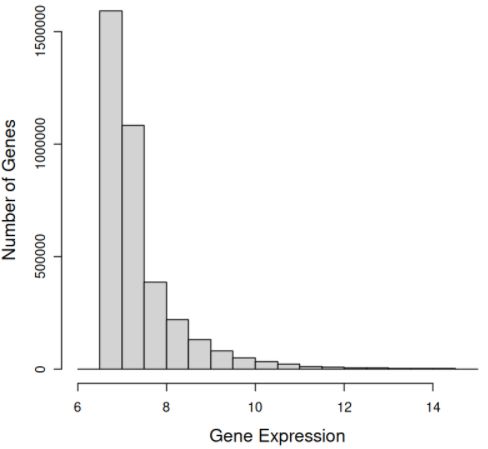
© Copyright 2022

Danielle Lambion
University of Washington Tacoma

                                                       Abstract

                         Treatment Response Prediction in Acute Myeloid Leukemia Patients

                                                  Danielle Lambion

                                         Chair of the Supervisory Committee:

                                               Professor Ka Yee Yeung
                                        School of Engineering and Technology

   Predicting acute myeloid leukemia (AML) patient treatment response has the potential to impact clinical decisions.

A prediction given at the time of diagnosis for treatment response can assist physicians in making effective treatment

decisions and improving patient prognosis. This project aimed to develop methods that leverage domain knowledge

in AML to identify biomarkers and build predictive models from biological datasets. Specifically, we applied our

methods to messenger RNA (mRNA) expression and gene mutation data extracted from bone marrow or peripheral

blood samples taken at patients’ time of diagnosis. Identified biomarkers are used as feature sets to train a prediction

model of patients’ treatment responsiveness. This prediction will aid physicians in optimizing treatment decisions for

patients on an individual basis.
ACKNOWLEDGMENTS
I want to thank Dr. Jerald Radich for providing this dataset and the opportunity to work on this project. I also want to
thank all my committee members for their incredible advice and support on this project. I especially want to thank
Dr. Ka Yee Yeung for her guidance throughout my thesis.
I would like to acknowledge Justin Guinney and Michael Mason at Sage Bionetworks, Erich Huang at Duke
University, and Linfang Deng at Shanghai University for sharing advice regarding our dataset.
2DEDICATION
Dedicated to my late father, René Lambion, whose support had allowed me to pursue my education.
3Contents
1 Introduction 8
2 Related Work 10
2.1 Gene Expression Correlation to Prognosis and Drug Response . . . . . . . . . . . . . . . . . . . . . 10
2.2 Gene Mutation Correlation to Prognosis and Drug Response . . . . . . . . . . . . . . . . . . . . . . 11
2.3 Machine Learning for Response Prediction . . . . . . . . . . . . . . . . . . . . . . . . . . . . . . . 11
3 Data and Methods 14
3.1 Problem Description . . . . . . . . . . . . . . . . . . . . . . . . . . . . . . . . . . . . . . . . . . . 14
3.2 Dataset . . . . . . . . . . . . . . . . . . . . . . . . . . . . . . . . . . . . . . . . . . . . . . . . . . 14
3.3 Data Processing . . . . . . . . . . . . . . . . . . . . . . . . . . . . . . . . . . . . . . . . . . . . . . 17
3.3.1 Preliminary Processing and Results . . . . . . . . . . . . . . . . . . . . . . . . . . . . . . . 17
3.3.2 Bead-Level Processing . . . . . . . . . . . . . . . . . . . . . . . . . . . . . . . . . . . . . . 17
3.3.3 Probe-Level Processing . . . . . . . . . . . . . . . . . . . . . . . . . . . . . . . . . . . . . . 18
3.4 Feature Selection . . . . . . . . . . . . . . . . . . . . . . . . . . . . . . . . . . . . . . . . . . . . . 19
3.5 Mutation Data . . . . . . . . . . . . . . . . . . . . . . . . . . . . . . . . . . . . . . . . . . . . . . . 19
3.6 Prediction . . . . . . . . . . . . . . . . . . . . . . . . . . . . . . . . . . . . . . . . . . . . . . . . . 20
3.7 Assessment . . . . . . . . . . . . . . . . . . . . . . . . . . . . . . . . . . . . . . . . . . . . . . . . 20
4 Results 22
4.1 Overview . . . . . . . . . . . . . . . . . . . . . . . . . . . . . . . . . . . . . . . . . . . . . . . . . 22
4.2 Exploratory Data Analysis . . . . . . . . . . . . . . . . . . . . . . . . . . . . . . . . . . . . . . . . 22
4.3 Processing Bead Array Data . . . . . . . . . . . . . . . . . . . . . . . . . . . . . . . . . . . . . . . 26
4.4 Differential Expression and Gene Set Enrichment . . . . . . . . . . . . . . . . . . . . . . . . . . . . 28
44.5 Mutation Data . . . . . . . . . . . . . . . . . . . . . . . . . . . . . . . . . . . . . . . . . . . . . . . 28
4.6 Prediction . . . . . . . . . . . . . . . . . . . . . . . . . . . . . . . . . . . . . . . . . . . . . . . . . 30
5 Conclusions 34
5List of Figures
3.1 Illumina Beadchip Technolgy [28] . . . . . . . . . . . . . . . . . . . . . . . . . . . . . . . . . . . . 16
3.2 Example outlier plot visualizing an artefact in the bead array surface . . . . . . . . . . . . . . . . . . 18
3.3 Example of control probe value intensity . . . . . . . . . . . . . . . . . . . . . . . . . . . . . . . . . 18
4.1 Bar plot of tissue sample type of responders and non-responders . . . . . . . . . . . . . . . . . . . . 23
4.2 Bar plot of sex of responders and non-responders . . . . . . . . . . . . . . . . . . . . . . . . . . . . 23
4.3 Bar plot of race of responders and non-responders . . . . . . . . . . . . . . . . . . . . . . . . . . . . 24
4.4 Bar plot of responders and non-responders in each protocol type . . . . . . . . . . . . . . . . . . . . 24
4.5 Density plot of patient age at diagnosis . . . . . . . . . . . . . . . . . . . . . . . . . . . . . . . . . . 25
4.6 Density plot of patient survival time . . . . . . . . . . . . . . . . . . . . . . . . . . . . . . . . . . . 25
4.7 Distribution of normalized probe-data . . . . . . . . . . . . . . . . . . . . . . . . . . . . . . . . . . 26
4.8 Distribution of gene-level expression data . . . . . . . . . . . . . . . . . . . . . . . . . . . . . . . . 27
4.9 Distribution of amount of probes to gene . . . . . . . . . . . . . . . . . . . . . . . . . . . . . . . . . 27
4.10 Heatmap of differentially expressed genes including annotations of mutations associated with response 30
4.11 Most important differentially expressed genes in model training from fold 2 during 5-fold cross-
validation . . . . . . . . . . . . . . . . . . . . . . . . . . . . . . . . . . . . . . . . . . . . . . . . . 31
4.12 Most important differentially expressed genes in model training across 5-fold cross-validation . . . . 33
6List of Tables
4.1 Genetic mutations found to be significantly associated with response by chi-squared tests. Gene mu-
tations associated with responsiveness to the induction treatment are shown in green and mutations
associated with non-responsiveness are shown in red. . . . . . . . . . . . . . . . . . . . . . . . . . . 29
4.2 Performance and number of features of the random forest model across a stratified 5-fold cross-
validation. . . . . . . . . . . . . . . . . . . . . . . . . . . . . . . . . . . . . . . . . . . . . . . . . . 31
7Chapter 1
Introduction
Leukemia is a cancer of the hematopoietic (blood) system. Acute myeloid leukemia (AML) specifically begins in the
bone marrow and can quickly spread to the blood. It is possible for AML to spread to other organs as well [6, 31].
AML is cured in 35% to 40% of patients 60 years or younger and 5% to 15% in patients over 60. The decreased respon-
siveness in elderly patients is often attributed to elderly patients being unable to receive more intensive chemotherapy
without significant side effects [6].
The genetic characteristics of an AML patient can be used to identify whether a patient will be responsive or non-
responsive to standard AML cancer treatment protocols [36, 43]. Publications have shown differentially expressed
genes can be used as predictive features. Zhang et al. showed genes, SLC17A7, MSX2, CDC26, MSLN, CTSZ and
DEFA3AML, were predictive of complete remission in childhood AML [43]. Similarly, Walker at al. developed a pre-
dictive model with NRP1, PLCB4, JMY, PSD3, DEXI, GAS6, C10orf55, AC139769.2, AC015712.2, and AL096865.1
gene expression for relapse in adults with AML [36]. Certain genetic mutations have been found to associate with
patient prognosis and the need for certain therapies to improve prognosis. Prior studies have found certain gene mu-
tations such as NPM1 and CEBPA mutations have been associated with improved responsive to standard treatment.
Other gene mutations have been associated with decreased responsiveness such as TP53 and ASXL1 [3, 6].
Precision medicine, also known as personalized medicine, is an approach that aims to personalize treatment and
care for medical patients based on their individual characteristics [9]. Precision medicine approaches have been applied
to treatment approaches involving cancer patients and more specifically in this thesis, acute myeloid leukemia (AML)
patients. Though AML is a heterogeneous disease, patients often undergo standard chemotherapy treatment. Studies
have shown improvements in overall survival when treatment was tailored from individual genomic profiles [1].
Big data projects have been generated to explore and understand the genomic landscape of AML. The Beat AML
8project from the Leukemia and Lymphoma Society aimed to study this genomic landscape and better match patients to
treatment from their individual genetic mutations. The Cancer Genome Atlas (TCGA) performed deep sequencing on
genomic data of patients and discovered 2,000 gene mutations from a dataset of 200 patients showing the heterogeneity
of this disease. Many of these genes have shown to correlate with prognosis. Tyner et al. reported their findings with
a dataset of 531 patients for comparison with findings from TCGA. Their findings showed many commonalities in
gene mutations. The Beat AML project focused on studying gene mutations’ effects on drug sensitivity. The results
showed many gene mutations or combinations of several mutations, did affect drug sensitivity. For example, the
IDH2 mutation correlated with sensitivity to many drugs, whereas IDH1 mutation correlated with resistance to many
drugs [33].
In this thesis, we designed machine learning models capable of predicting AML patient responsiveness to stan-
dard treatment protocols. Contributions of this thesis include processing and normalization of gene expression data,
identification of gene mutations and differentially expressed genes associated with treatment. We identified biological
pathways enriched among our differentially expressed genes and found pathways related to cancer. We also used these
differentially expressed genes as predictive features in machine learning models for patient response. Our predictive
model achieved comparable or better performance to recent publications in the literature [8, 43, 37].
9Chapter 2
Related Work
In this thesis, we identified differential gene expression and gene mutations associated with induction treatment re-
sponse for AML patients. Then, we used the differentially expressed genes associated with the treatment response
as features to train an induction treatment response prediction model for AML. In this chapter, we will discuss work
related to this thesis project in the literature. Specifically, we will review work that focused on identifying gene expres-
sion or gene mutation signatures associated with prognosis or drug response in AML. We will also discuss machine
learning models for cancer treatment response prediction.
2.1 Gene Expression Correlation to Prognosis and Drug Response
Patient gene expression profiles have been shown to predict prognosis and drug response [2, 21, 35]. Cucchi et
al. performed a study correlating gene expression profiles with drug response in pediatric AML patients. Patients
resistant to etoposide had lower expression levels across most of the gene set. Cucchi et al. also reported that Over-
expression in TFDP3 was associated with resistance to chemotherapy. Cytosine arabinoside response was associated
with high expression of KMT2B, KMT2D, and RBBP5. Expression levels of genes BRE, HIF1A, and CLEC7A were
also shown to exhibit significant associations with drug response [2]. Visani et al. performed a study on elderly AML
patients predicting the response of tosedostat and low-dose cytarabine. Gene expression of CD93, GORASP1, and
CSCL16 were shown to be associated with response to the drug regimen [35]. Nehme et al. calculated a prognostic
score with the weighted sum of the expression of 22 genes that are commonly deregulated (CODEGs). CODEGs were
shown to correlate with myeloid differentiation, leukemia stem cell status, and relapse [21].
102.2 Gene Mutation Correlation to Prognosis and Drug Response
Certain genetic mutations or combination of multiple mutations are known to have effects on patients’ response to
treatment and patients’ prognosis [7, 19, 32]. Elrhman et al. reported an impact on AML patient prognosis when
mutations of DNMT3A, FLT3, and NPM1 were concurrently present. AML patients with mutations of these three
genes had the worst prognosis, as opposed to other patients in the study with just one or two of the genes having
mutations. This is then followed by patients with a mutation in DNMT3A, then DNMT3A and FLT3, then DNMT3A
and NPM1. The study shows a negative affect of all three genes having mutations, as well as, a negative effect
when a mutation is present in DNMT3A [7]. Libura et al. found AML patients’ with IDH2 mutations had better
clincal outcomes with cladribine, daunorubicin, and cytarabine induction treatment, but not necessarily with other
treatments [19]. Tavor et al. found patients with FLT3-ITD and PTPN11 responded well to dasatinib, whereas,
patients with TP53 mutations responded poorly to the drug. Tavor et al. also performed RNA sequecing and found
unique gene expression profiles in combination with the mutations showed correlation to dasatinib sensitivity [32].
2.3 Machine Learning for Response Prediction
In this section, existing machine learning techniques and approaches for oncology are discussed. Specifically, we will
discuss chemotherapy drug response prediction by Huang et al [9]. Sakellaropoulos et al. proposed a neural network
for drug response and survival prediction with neural networks [30]. We will also discuss the work by Gal et al. that
explored several models to predict complete remission in AML patients [8]. Additionally, we discuss Lee et al.’s
MERGE algorithm [14].
Huang et al. proposed a support vector machine (SVM) model to predict cancer patients’ response to specific
treatment drugs. SVM recursive feature elimination (SVM-RFE) was the technique utilized for the task of feature
selection of gene expression in this model. Huang et al. acquired their gene expression dataset from the Cancer
Genome Atlas (TCGA). Huang et al. applied their methodology across 175 treatment drugs, which ranged in accuracy
of 81.5% to 82.6%. The model was trained and tested using a cross-validation approach across a dataset of 152 patients
with 32 types of cancer using a 75% train and 25% test split [9]. Huang et al.’s approach is similar to our approach, in
that we utilized gene expression to create feature model subsets. Similarly, our model predicted the responsiveness of
patient to treatment. Huang et al.’s approach differs in that it does not narrow its study to one form of cancer and the
responsiveness prediction is for individual treatment drugs. Our approach predicted the responsiveness to induction
treatment specifically for AML patients.
Sakellaropoulos et al. approach uses a deep neural network (DNN) to predict treatment drug response and survival
11of cancer patients using gene expression data. Their dataset was comprised of 55 different types of cancer from
1,001 cell line samples from the Genomics of Drug Sensitivity in Cancer (GDSC) database. Gene expression in
this database was sequenced using Affymetrix Human Genome U219 arrays. Sakellaropoulos et al. trained DNN,
random forest (RF), and ElasticNet models to compare results. Each model was trained on two sets of features: all
of the genes and the most variable genes. The most variable genes were determined by median absolute deviation.
Sakellaropoulos et al. reported notably higher area under the curve (AUC) with the DNN model over other model
types for predicting binary responsiveness, independent of the subset of genes selected as features. The AUC for the
DNN model mostly outperformed others as well in survival prediction, but sometimes was comparable to other models
dependent on the feature set [30]. Sakellaropoulos et al. predicted binary responsiveness of patients. Sakellaropoulos
et al. developed several models for individual treatment drugs and across various types of cancer. As mentioned
prior, our approach predicted binary responsiveness to induction treatment specifically for AML. Our work also did
not extend to prediction of patients’ survival or explore deep learning models as Sakellaropoulos et al.’s work did.
Sakellaropoulos et al. perform feature selection by measuring each gene’s median absolute deviation and selecting the
90% or 80% of most variable genes. We identified differentially expressed genes by fitting a linear model with the
LIMMA [29] package as feature selection.
Gal et al. proposed machine learning models to predict complete remission of AML patients using gene expression
data from RNA sequencing. Gal et al. dataset included 473 patients that are children or young adults. 414 patients
were in complete remission. Gal et al. used the t-test to identify the 100 most differentially expressed genes. The
differentially expressed genes were used to train k-nearest neighbors (k-NN), SVM, and RF models to perform further
feature selection. The k-NN model used Randomized Lasso and Hill Climbing feature selection methods. SVM-
RFE was also used and a ranking of feature importance was derived from the RF. The model resulting in the highest
AUC using the top 50 genes, k-NN with K=27 and Hill Climbing, was selected at an AUC of 84% evaluated on a
test dataset [8]. Gal et al. used a different feature selection approach for each model. K-NN used a t-test to intially
select differentially expressed genes. For subsequent folds, Hill Climing and Randomized Lasso were both used, the
AUC was computed on the subset of selected genes and genes were ranked by the average of AUCs using those genes
across different folds. A similar approach was used for the SVM classifier, except Recursive Feature Elimination was
added. The RF classifier used two approaches to feature selection. The first trained each fold on the entire feature
set to acquire the feature importances. The model was then retrained with the most important features with the same
fold. The second approach performed 100 iteration of 5-fold cross-validation and aggregating the feature importance
values during each fold. The correlation was then calculated between each gene’s importance and the AUC in every
fold. Genes with the highest importance scores were selected. Gal et al.’s approach is very similar in that we predicted
12patients’ responsiveness to induction treatment. We defined a patient that is responsive as in complete remission in
our dataset as well. A key difference is that our dataset does not include children, but includes a range of patients
from young adult to elderly. We focused on patients that did not respond at all to treatment or that achieved complete
remission for at least 2 years, though some may have relapsed late. Our feature selection method was most similar
to Gal et al.’s method for the SVM classifier in that we selected differentially expressed genes as our features. We
differed in our approach for identifying differentially expressed genes by fitting a linear model with gene expression
using the LIMMA package.
Lee et al. proposed a computational method, MERGE (mutation, expression hubs, known regulators, genomic
CNV, and methylation), to identify gene expression biomarkers by integrating prior, relevant multi-omic information.
MERGE learns from TCGA’s AML study’s mutation data, hubness of a gene expression network derived from public
datasets, the gene’s role from gene annotation databases, genomic copy number variation (CNV) data from TCGA’s
AML study, and methylation data from TCGA’s AML study. A gene’s biomarker potential weight is calculated from a
combination of those features. Genes scored highly by MERGE tend to have correlations with drug sensitivities. Lee
et al. tested the MERGE algorithm on a dataset of 30 AML patients across 62 treatment drugs. MERGE was compared
to other models that predicted drug response: ElasticNet, multi-task learning, and Bayesian multi-task multiple kernel
learning (MKL). MERGE outperformed the other 3 models on 62% of drugs in the dataset. MERGE also found
eight highly ranked genes with biological significance to AML: FLT3, CASP8AP2, L2HGDH, MNT, BAZ2B, MZF1,
BEX2, and SMARCA4 [14]. Our work differed from MERGE in that we predicted response to induction treatment
received after initial diagnosis. Our dataset does not provide information on individual treatment drugs received by
patients. MERGE calculates a score for a gene based off 5 features for each gene: mutation, expression hubness,
whether it has a known Regulatory role, genomic CNV, and methylation. This requires prior knowledge of these
features’ association with AML and previous studies’ data to generate feature weights. We identified differential gene
expression to be used as features in our predictive model. Our approach does not require prior knowledge or integration
of previous studies’ datasets.
13Chapter 3
Data and Methods
3.1 Problem Description
We developed genetic feature selection methods that yielded prediction models of AML patients’ treatment response.
We focus on a binary prediction problem, where a patient is predicted as responsive or non-responsive to the induction
treatment protocol. This problem requires identifying biomarkers of patients’ response to treatment from mRNA
expression and gene mutation data. In this thesis, we processed raw gene expression data, applied statistical methods
to identify differentially expressed genes and gene mutations, and subsequently evaluated the best features predictive
of treatment response. This approach can be broken into the following tasks:
• Data pre-processing, exploration, and cleaning
• Identification of biomarkers and feature selection
• Training and evaluation of predictive models
This project focused on the analysis of genomics data and development of machine learning models to predict
patient treatment response. The software utilized in this thesis included R [25], Bioconductor [10] packages such as
Subread [16], BedTools [24], Python3 [34], and Scikit-Learn [23].
3.2 Dataset
The data used for this project was generated by the Radich Lab at the Fred Hutchinson Cancer Research Center. This
dataset contains information for 198 AML patients. Clinical data, mRNA expression data, and gene mutation data
14is supplied for each patient. Most AML patients respond to treatment, then relapse [42]. This dataset is unique in
that it was generated from outlier patients’ samples. Meaning this dataset contains samples of patients who do not
respond to the induction treatment and patients who achieve complete remission with the induction treatment and do
not relapse within the followup period of at least two years. All patients within this datatset are cytogenetically normal,
meaning these patients’ AML is not associated with significant chromosomal abnormalities [20]. This helps reduce
the heterogeneity of the dataset.
The clinical data includes eleven attributes: diagnosis, collection event, tissue type, AML response category,
material type, race, sex, survival time, protocol, age at collection, and handling note. The diagnosis, collection event,
and material type are the same for every patient. The diagnosis is AML, the collection event was taken at the time
of diagnosis, and the material type is RNA. Race is a categorical feature, where possible categories are black, white,
Asian Pacific Islander, other, or unknown. Sex is a binary feature of either female or male. Survival time is a numerical
feature describing the number of days from diagnosis to death. Survival time is non-applicable to surviving patients.
Protocol is a categorical feature referring to the treatment protocol for a given patient. Age refers to patients’ age at
diagnosis. The handling note provides information on collection batch. The AML response category serves as our
binary label of responsive to treatment or non-responsive to treatment. Responsive patients are defined as patients
that had continued complete remission for over two years. Non-responsive patients are defined as patients that did not
achieve complete remission from induction therapy. This dataset is comprised of 83 responsive and 115 non-responsive
patients.
The gene expression data was generated using the Illumina HumanHT-12v4 beadchip array containing 48,107
probe identifiers per experiment. The patients’ tissue samples are scanned with the beadchip array. Each bead on
the beadchip is coated with multiple copies of probes to ensure robust measurements for the probe-level data. The
summary-level data summarizes the expression probe values on the beadchip for each probe or each gene as shown
in Figure 3.1. Probes on the beadchip target the expression of a specific location in the genome. In this context, each
experiment represents a patient sample, resulting in an array where columns are patient identifiers and rows are the
numerical expression value for each probe. Each probe is designed to target specific transcripts in the genome. Our
goal is to determine the mRNA level of each transcript, therefore the probes’ identifier number will be mapped to a
corresponding gene or transcript. Note that multiple probes could be mapped to the same gene or transcript. 63.2% of
genes had a one-to-one probe to gene mapping, while 36.8% of genes had multiple probes map to them.
15Figure 3.1: The design of the Illumina beadchip array technology. Each bead on the beadchip is coated with multiple
copies of probes to ensure robust measurements for the probe-level data. The summary-level data summarizes the
expression probe values on the beadchip for each probe or each gene [28].
The gene mutation data includes mutation information for 180 genes. Each patient may have a single mutation,
multiple types of mutations, or no mutation at all in a given gene. A gene mutation occurs when the DNA contained
within a gene is altered in some way. There are multiple DNA variations that can occur causing gene mutations. We
focused on missense and frameshift mutations. A missense mutation occurs when there is a change in a single base
that results in a codon for a different amino acid. Frame shifts occur when a base is either deleted or inserted in the
coding sequence. There are two types of frameshift mutations, frameshift by deletion and frameshift by insertion. Due
to a single base being inserted or deleted, instead of changing a single codon, the genetic sequence shifts and produces
different amino acids following the deletion or insertion [12].
163.3 Data Processing
3.3.1 Preliminary Processing and Results
We mapped probe identifiers to genes to identify differentially expressed genes (i.e., genes that exhibit different activity
patterns across responders versus non-responders). The dataset was generated several years ago and we found that the
available Bioconductor annotation, illuminaHumanv4.db [4], no longer accurately annotates this dataset and could not
provide annotations to 29.38% of probe identifiers. Due to this, we adopted the strategy of creating our own mapping
between probes and transcripts using the probe sequences on the beadchip. Specifically, we mapped probe identifier
with the A-MEXP-2088 array design [39] for the Illumina HumanHT-12V4 beadchip with the addition of an extra
probe, ILMN_2044813, to derive each probe’s gene sequence. The A-MEXP-2088 array design file provides each
probe and the genetic sequence read by that probe. We explored other array files for the Illumina HumanHT-12V4
beadchip and found this was the file able to match 100% of our probe identifiers to a gene sequence. Then, we used the
Bioconductor package, Subread [16], to align the derived gene sequences from the A-MEXP-2088 design file against
the human genome. BedTools [24] was used to intersect this data with the corresponding bed file, a file where each
row contains the chromosome, start and end positions of the chromosome, and the gene symbol, to create a file of
probe identifier to gene mapping. In this mapping, a gene may have one or multiple probe identifiers mapped to it.
We summarized any genes that were mapped from multiple probes with three methods: median, mean, and geo-
metric mean. This resulted in a single expression value for each gene across patients. We then performed t-tests with
the Bonferroni p-value adjustment to correct for multiple comparison with a p-value threshold of 0.05 to determine
differential gene expressions between responders and non-responders. This resulted in no differential genes across
all methods for the pre-normalized data. This is likely due to over-normalization as we saw little variation across the
expression values or due to the conservative nature of the Bonferroni adjustment.
3.3.2 Bead-Level Processing
Given the lack of signal in our preliminary results, we used the beadarray [5] Bioconductor package to convert the
bead-level data to probe-level data, remove outliers, and experiment with different normalization methods. The beadar-
ray package allows for bead-level analysis and quality assessment of Illumina beadarray datasets.
17Figure 3.2: Example of an outlier plot visualizing a bead array’s surface with an artefact present in the array surface
of sample 5243. Outlier plots indicates below median outliers in blue and above median outliers in pink. This sample
has a spatial artefact in the left side of the chip, where there are values missing in the white line.
Prior to converting the bead-level data to probe-level, we performed quality assurance data analysis by visually
inspecting images of bead arrays. Boxplots of green intensity values were visually checked for inconsistencies. The
boxplots across all samples were similar and also appeared consistent when compared to example Illumina beadarray
data provided by beadarray’s vignette. Outlier plots were used to visualize the array surface for each sample. 20
samples were identified as having artefacts, such as in Figure 3.2, in the array’s surface. We plotted the log-based
intensity of the control probes. Control probes are expected to have high intensity values. Control probe 450292 had
lower intensity values as seen in Figure 3.3, but this was consistent across all samples in this dataset. The other control
probes had high expression across all the samples. No samples were removed due to quality assurance assessed by
plotting the control probes. The beadarray package was used to then summarize the bead-level data into probe-level
data.
Figure 3.3: Example of intensity values of control probes for samples 5036, 5045, and 5054. Housekeeping control
beads are shown in red and biotin control beads are shown in blue. These 3 samples were randomly chosen as all
samples are similar across the dataset.
3.3.3 Probe-Level Processing
We removed the 20 samples identified as having artefacts after having summarized to probe-level and performed quan-
tile normalization on the samples. We performed quality assurance again by checking the Illumina probe annotation
quality. Probe annotation quality is measured by comparing the transcript the probe read against its target transcript,
18the genetic sequence the probe should match. Beadarray classifies annotation qualities as ’Perfect’, ’Good’, ’Bad’,
or ’No Match’. 12,379 bad probe annotations and 1,252 unmatched annotations were dropped from the dataset. This
results in removing 28.3% of the probe data.
We summarized our probe-level expression data to gene-level data using three different methods: mean, median,
and geometric mean across all probes in each gene. We later compared results found by these three methods by t-tests
as described in Section 3.4. We found mean and geometric mean identified the same 31 differentially expressed genes,
while median found 30. The 30 found by the median were also contained in the sets found by mean and geometric
mean. Mean was chosen as the summary method for subsequent analysis in this thesis. We used the same probe to
gene mapping generated in Section 3.3.1 to accomplish this.
3.4 Feature Selection
We began feature selection with a univariate method to discover differentially expressed genes. This is the same two-
sided t-tests as used in the pre-normalized mRNA expression data. We considered genes with a p-value less than 0.05
as differentially expressed after using Bonferroni correction for multiple comparisons. We performed the t-tests across
all three gene-level data: mean, median, and geometric mean described in Section 3.3.3. We also used Linear Models
for Microarray Data (LIMMA) [29] to identify differences between mean gene expression. As the name suggests,
LIMMA fits a linear model and computes contrasts. LIMMA uses Benjamini-Hochberg adjustment with a 0.05 p-
value threshold. We performed Gene Set Enrichment Analysis with Enrichr [40] to identify pathways and functional
categories associated with response to treatment on the differentially expressed gene set identified with LIMMA. We
worked closely with Dr. Radich and Dr. Appelbaum to identify biologically relevant genes and interpret pathway
results.
3.5 Mutation Data
We performed a chi-squared test across mutation data to find significant mutations in genes associated with response.
To perform this, we used a matrix for each mutation type. A 1 in the matrix denoted a mutation present and 0 denoted
no mutation. A p-value of less than 0.05 is considered associated with response. We then performed correlation tests
with Pearson correlation between the gene expression data and mutation data. Both of these tests are utilized from the
stats package [26]. Pearson correlation computes a coefficient that indicates how much two variables are correlated.
We correlated each vector of a gene mutation with each vector of a gene’s expression data from samples that had gene
mutation data available.
193.6 Prediction
We trained a random forest [17] model using genetic biomarkers as features. Our random forest model uses 120
estimators and Gini index as the splitting criterion. To evaluate our model, we performed an 80% training and 20% test
split across a 5-fold cross-validation with stratification. For each training and testing split, we derived the differentially
expressed genes again using LIMMA as described in Section 3.4. The set of differentially expressed genes derived
from the current fold’s training set become the features used for training and testing. We used metrics described in
Section 3.7 to assess our model’s performance. Deriving feature importances from each fold allowed us to discover
which features add value to the prediction model by comparing which features are ranked as important across every
fold. Feature importance values are calculated by each features’ node’s impurity within the decision trees and weighted
by the number of samples that reached that node during training.
3.7 Assessment
We utilized accuracy and area under the curve (AUC) to measure the performance of our trained model. We took these
measurements across a 5-fold cross-validation with stratification. We also derived feature importances from each fold
to compare features that are consistently predictive of patient responsiveness. Stratification of the folds allowed us to
have the same ratio of responders and non-responders in each fold as the original, full dataset.
Metric 1: Accuracy
This metric calculates the percentage of how often the model correctly predicts new classification instances.
TP + TN
Accuracy =
TP + TN + FP + FN
T P = T rue P ositive
F P = F alse P ositive
T N = T rue N egative
F N = F alse N egative
Metric 2: AUC
This metric quantifies how well our model separates the two classification classes. An area under the ROC
curve (AUC) of 50% shows absolutely no class separation. Whereas, an AUC of 100% shows the two classes
20are entirely distinguished from one another. AUC is calculated by plotting the TPR (y-axis) against the FPR
(x-axis). The AUC is the integral of this plotted curve.
21Chapter 4
Results
4.1 Overview
In this chapter, we will discuss analysis and results found during this project. Specifically, we explored the clinical
data of patients who are responders versus non-responders. In this thesis, we focused our effort on gene expression
data generated using the Illumina beadarray technology. This technology and methods used to process the raw data
were described in Chapter 3. We will report the results of data processing and normalization in this chapter. Using the
summarized and normalized gene expression, we identified differential expressed genes with two different methods.
Subsequently, we inferred gene categories enriched in these differentially expressed genes. Additionally, we applied
machine learning methods to build models predictive of treatment response. Finally, we will report different types of
gene mutations associated with response.
4.2 Exploratory Data Analysis
We performed data exploration of clinical data of patients. In particular, we aim to investigate the distributions of
different clinical variables with respect to responders versus non-responders. We observe in Figure 4.1 that the tissue
sample type (i.e. bone marrow versus blood) is not associated with the response to therapy. In Figure 4.2, we observe
that more female patients had been responsive to treatment. In terms of race, we observe that the majority of the
patients are white or have unknown racial groups as seen in Figure 4.3. Unknown is the second largest category for
race in our dataset and does not allow us to infer much information about that group. We can view which treatment
protocols were more effective for patients responsiveness than others in Figure 4.4. Treatment protocols indicate which
22cancer research cooperative group treated the patient and the treatment regimen received. Some treatment protocols
had a significantly higher number of responsive patient, like Cancer and Leukemia Group B (CALGB) 19808 and
others had overwhelming numbers of non-responsive patients, like Eastern Cooperative Oncology Group (ECOG).
We observe that the mean age of responsive patients is slightly younger than non-responsive patients as expected in
Figure 4.5, but there is not much separation between the classes across patient age. Figure 4.6 shows that the survival
time of non-responsive patients is significantly less than responsive patients as we would expect as well.
Figure 4.1: Number of responsive and non-responsive
Figure 4.2: Number of responsive and non-responsive
patients by tissue sample type collected from the full
patients by sex from the full dataset of 198 patients. Female
dataset of 198 patients. The sample type has no
patients tend to respond more often to treatment.
association to treatment response.
23Figure 4.3: Number of responsive and non-responsive patients by race from the full dataset of 198 patients. We
cannot infer much about race as unknown is the second largest category. White patients patients are the majority of
the dataset. It is difficult to infer information about race’s association with response.
Figure 4.4: Number of responsive and non-responsive patients by treatment protocol type from the full dataset of
198 patients. Treatment protocols indicate which cancer research cooperative group treated the patient and the treat-
ment regimen received. Some protocols had large numbers of responders, such as Cancer and Leukemia Group B
(CALGB) 19808, CALGB 9621, and Southwest Oncology Group (SWOG) s9034. Eastern Cooperative Oncology
Group (ECOG) has a significantly larger number of non-responders than other protocols.
24Figure 4.5: Patient age at the time of diagnosis separated by responder and non-responder class labels from the full
dataset of 198 patients. The x-axis denotes patient age and the y-axis denotes the kernel density estimate. The kernel
density estimate shows a smoothed histogram of the data. The blue dashed line denotes the mean age of responders,
while the red dashed line denotes the mean age of non-responders. There is not much separation in patient ages across
the two groups. The mean age of responders being slightly lower is as expected.
Figure 4.6: Survival time of patients separated by responder and non-responder class label after removal of non-
applicable, surviving patients from the full dataset of 198 patients. Survival time is the number of days after the
time of diagnosis. The x-axis denotes patient survival time and the y-axis denotes the kernel density estimate. The
kernel density estimate shows a smoothed histogram of the data. The red dashed line is the mean survival time of
non-responders, while the blue dashed line is the mean survival time of responders. The survival time is significantly
shorter for non-responders as expected.
254.3 Processing Bead Array Data
We removed the noise from the dataset by conducting the analysis described in Section 3.3.2. Dropping samples
with artefacts resulted in 178 patient samples, of which 74 are non-responders and 104 are responders. In Figure 4.7,
we observe the distribution of probe-level expression. The probe-level expression values have a right-skewed normal
distribution, where the majority of probes have lower expression values. Figure 4.8 depicts a similar distribution of the
gene expression values. Observing the ratio of probes to genes in Figure 4.9, we expected this similar right-skewed
distribution as most genes have a one-to-one ratio to probes. This is important for t-tests as we must assume a normal
distribution in the two groups: responders and non-responders.
Figure 4.7: This histogram shows the distribution of the quantile normalized probe values for 178 patient samples
after removing samples with artefacts. The distribution was right-skewed with most probe expression values around 7.
26Figure 4.8: This histogram shows the distribution of gene expression values summarized by mean from the probe-
level data for 178 patient samples after removing samples with artefacts. This distribution was similarly right-skewed
as to the distribution of probe values. Most gene expression values were around 7.
Figure 4.9: This histogram shows the distribution of the amount of probes that match to each gene. Most genes had
a single probe value and just over 400 genes had 2 probe values. 42 genes, a small number of our dataset’s 20,462
genes, had over 12 probes per gene and are not depicted in this graph.
274.4 Differential Expression and Gene Set Enrichment
We used the t-test and LIMMA described in Section 3.4 to determine a set of differentially expressed genes between
responders and non-responders. Mean was used to summarize any genes that were mapped from multiple probes
for these results. We identified 31 differentially expressed genes by t-test and 788 differentially expressed genes
with LIMMA. We compared the two lists of differentially expressed genes and found that all 31 differentially ex-
pressed genes from the t-test were also found within the 788 discovered by LIMMA. The 31 identified differentially
expressed genes’ expressions by t-test are visualized in Figure 4.10. The heatmap visualizes the expression differ-
ence between non-responders and responder. For example, we observe MARK2P10 has some responders with lower
expression values, while non-responders have consistently high expression values. ZNRD1ASP_6 has a number of
non-responders with high expression values, while the majority of responders have low expression. We idenfitied
the gene expression of MARK2P10, CCT4P1, C2orf81, HMGA1P8, ZNRD1ASP_6, ACTG2, NIPBL, LINC00654,
KIR2DL5A_4, TRO, C11orf65, ATM, TRIM80P, RRBP1, LOC400464, CPLANE1, TAFA1, KCNA5, TMEM200A,
PROCA1, MRPS18A, SRP9P1, TNKS2, PPIP5K2, and DDX25 to be associated with not responding to the induction
treatment. Gene expression of TMEM126A, LINC00690, TUBB7P, CNGA3, PRORY, and LRRC74A was associated
with responsiveness.
We performed gene set enrichment analysis (GSEA) with the 788 genes identified with Enrichr [40] and analyzed
results with the insights of Dr. Jerald Radich and Dr. Jacob Appelbaum. We looked at pathways our identified genes
matched with in the Kyoto Encyclopedia of Genes and Genomes (KEGG) [11] and Molecular Signatures Database
(MSigDB) [18] pathway databases. Glycolysis is a significant pathway discovered by our differentially expressed
gene set in KEGG and IL-2/STAT5 signaling pathway in MSigDB. Glycolysis can induce T cell dysfunction and
is known as a hallmark of cancer. Glycolysis is also a known major pathway in another type of leukemia, chronic
myeloid leukemia [27]. This relates to the IL-2/STAT5 signaling pathway, as IL-2/STAT5 signaling is related to T cell
activation. Ferroptosis is another pathway found, but had a p-value significance of 0.077. Ferroptosis is still noteable
here as it is a type of cell death induced by gene P53 [15].
4.5 Mutation Data
We performed a chi-squared test as described in Section 3.5 to discover mutations in association with response. Seven
genes were found to be significantly associated with response, one of which was significant in two different mutation
types. We can see these mutations described in Table 4.1. The mutations identified as associated with response are
known within the literature [22, 44]. These identified genes are visualized between responders and non-responders in
28Figure 4.10. In this visualization, we observe the differences between the number of mutations found in each gene
across responders and non-responders. Non-responders have some gene mutations in non-responders, but none in
responders. We associate this gene mutation with poor response to treatment. IDH2 can be associated with better
response to treatment, having more mutations found in responders.
Mutation Type Description Genes
Frameshift by deletion A shift in the DNA sequence caused DNMT3A
by deletion of one or more bases [12]
Frameshift by insertion A shift in the DNA sequence caused NPM1
by insertion of one or more bases [12]
Missense A change in a single base that results CMYA5, HMCN1, IDH2,
in a codon of a different amino acid [12] NPM1, and RUNX1
Table 4.1: Genetic mutations found to be significantly associated with response by chi-squared tests. Gene mutations
associated with responsiveness to the induction treatment are shown in green and mutations associated with non-
responsiveness are shown in red.
29Figure 4.10: Heatmap of the 31 differentially expressed genes found by t-test with Bonferroni correction and a
threshold of 0.05. Red denotes higher mRNA expression levels, while lower expression levels are shown in blue. The
intensity of the color relates to the level of expression. The columns are patient samples and the rows are the genes.
The expression columns were split by their label, then clustered separately within that label. The rows were clustered
across all expression samples. In MAR2P10, there were lower expression values in responders, but only high values
in non-responders showing expression differences across the two groups. The bottom annotation shows mutations
associated with response found by the chi-squared test and a threshold of 0.05. Red in the mutations denotes one
or more mutations were present in that gene, while purple denotes no mutations were present. A gene mutation in
CMYA5 was associated with not responding to treatment, as no mutations were found in responders. IDH2 mutations
were associated with being responsive to treatment, as more mutations were found in responders. The left annotation
shows the p-value found by t-test with Bonferroni correction for each gene.
4.6 Prediction
The random forest model is trained and evaluated as described Section 3.6. There is a significant variation in the
number of features selected between the training sets selected across each fold. In Table 4.2, Fold 5 is the worst
performing model and selected the largest number of differentially expressed genes as features. Fold 2 had the highest
30accuracy and the smallest number of selected features. Selecting a small set of predictive features helps improve
the predictive model’s performance, as opposed, to simply selecting more features. We then performed a 10-fold
cross-validation, which achieved a similar average performance of 71.08% accuracy and 78.71% AUC.
Fold Accuracy AUC Number of Features
1 72.22% 75.71% 931
2 83.33% 86.51% 55
3 77.77% 87.94% 198
4 82.86% 81.33% 190
5 51.43% 59.86% 1142
Average of All Folds 73.52% 78.27% N/A
Table 4.2: Performance and number of features of the random forest model across a stratified 5-fold cross-validation.
Figure 4.11: Feature importance of the 55 differentially expressed genes used as features in fold 2 of the 5-fold
cross-validation of the random forest. Feature importance was calculated by each features’ node’s impurity within the
decision trees and weighted by the number of samples that reached that node during training. The closer a feature
importance is to zero, the less informative that feature is to the model. These 55 genes were identified with the 80%
training portion selected by fold 2 using LIMMA and an adjusted p-value threshold of 0.05. LINC00654 was found to
be significantly more predictive of response than other differentially expressed genes.
The feature importances were derived as described in Section 3.6. We graphed these importances to visualize the
amount of impact selecting certain gene’s had on a model’s predictive ability. Figure 4.11 visualized features from
fold 2, the best performing fold in accuracy, and close to the best performing fold in AUC at 1.43% less than fold 3.
LINC00654 had a significantly larger impact on the model’s prediction than any other feature selected.
Figure 4.12 depicts the 20 most important features in each fold. LINC0654 was the most important predictor of
responsiveness in every fold, except fold 4, where LINC0654 was the sixth most important predictor. Fold 4 found
NIPBL to be the most important predictor. Other genes were important predictors across several folds, such as, NIPBL.
31NIPBL appeared in the top 13 most important features throughout all folds, except fold 1.
32(a) The 20 most important differentially expressed (b) The 20 most important differentially expressed
genes used as features in fold 1. genes used as features in fold 2.
(c) The 20 most important differentially expressed (d) The 20 most important differentially expressed
genes used as features in fold 3. genes used as features in fold 4.
(e) The 20 most important differentially expressed genes used as features in fold 5.
Figure 4.12: The 20 most important differentially expressed genes used as features throughout each fold in the 5-
fold cross-validation of the random forest. The differentially expressed genes used as features in each fold were
re-identified by LIMMA with an adjusted p-value threshold of 0.05. LINC0654 was the most important predictor of
responsiveness in every fold, except fold 4, where LINC0654 was the sixth most important predictor. NIPBL was also
found as predictive of response by each model, except fold 1.
33Chapter 5
Conclusions
In conclusion, we successfully analyzed and cleaned the mRNA gene expression dataset of noise. We identified
differentially expressed genes associated with AML response. Our discovered gene set is novel and unique from those
found in the literature. This is likely due to the sample selection applied to this dataset, where patients who responded
to induction treatment, then relapsed within the two year follow-up period were omitted from the dataset. We trained
and evaluated a random forest model and achieved comparable performance to what is being published in the literature
using our differentially expressed gene selection methods for features. We have identified a small number of genes
found to be predictive of responsiveness.
This work can be expanded upon. The identified gene mutations associated with response can be combined as
features within our models. Gene mutation and gene expression correlation can be used to discover which gene
expressions are independently predictive of response. We can also include clinical variables as features, such as
patient age. The evaluation of the models can be expanded by validating on other AML datasets such as Beat AML
or other available data from studies in the literature [13, 38]. These datasets could also be combined and evaluations
performed could be repeated. Other methods for feature selection and training could be explored such as iterative
Bayesian Model Averaging [41].
34Bibliography
[1] Precision Medicine Feasible in AML. Cancer discovery, 2020.
[2] D.G.J Cucchi, Costa Bachas, Marry Heuvel-Eibrink, Susan Arentsen-Peters, Zinia Kwidama, Gerrit Jan Schu-
urhuis, Yehuda Assaraf, Valerie Haas, Gertjan Kaspers, and Jacqueline Cloos. Harnessing gene expression
profiles for the identification of ex vivo drug response genes in pediatric acute myeloid leukemia. Cancers,
12(5):1247, 2020.
[3] Courtney D DiNardo and Jorge E Cortes. Mutations in aml: prognostic and therapeutic implications. Hematol-
ogy, 2016(1):348–355, 2016.
[4] Mark Dunning, Andy Lynch, and Matthew Eldridge. illuminaHumanv4.db: Illumina HumanHT12v4 annotation
data (chip illuminaHumanv4), 2015. R package version 1.26.0.
[5] Mark J. Dunning, Mike L. Smith, Matthew E. Ritchie, and Simon Tavaré. beadarray: R classes and methods for
Illumina bead-based data. Bioinformatics, 23(16):2183–4, 2007.
[6] Hartmut Döhner, Daniel J Weisdorf, and Clara D Bloomfield. Acute myeloid leukemia. The New England
journal of medicine, 373(12):1136–1152, 2015.
[7] Heba Allah E Abd Elrhman, Yomna M El-Meligui, and Saffaa M Elalawi. Prognostic impact of concurrent
dnmt3a, flt3 and npm1 gene mutations in acute myeloid leukemia patients. Clinical lymphoma, myeloma and
leukemia, 2021.
[8] Ophir Gal, Noam Auslander, Yu Fan, and Daoud Meerzaman. Predicting complete remission of acute myeloid
leukemia: Machine learning applied to gene expression. Cancer Informatics, 18:1176935119835544, 2019.
PMID: 30911218.
[9] Cai Huang, Evan A Clayton, Lilya V Matyunina, L DeEtte McDonald, Benedict B Benigno, Fredrik Vannberg,
35and John F McDonald. Machine learning predicts individual cancer patient responses to therapeutic drugs with
high accuracy. Scientific reports, 8(1):16444–8, 2018.
[10] Wolfgang Huber, Vincent J. Carey, Robert Gentleman, Simon Anders, Marc Carlson, Benilton S. Carvalho, Hec-
tor C. Bravo, Sean Davis, Laurent Gatto, Thomas Girke, Raphael Gottardo, Florian Hahne, Kasper D. Hansen,
Rafael A. Irizarry, Michael Lawrence, Michael I. Love, James MacDonald, Valerie Obenchain, Andrzej K. Oleś,
Hervé Pagès, Alejandro Reyes, Paul Shannon, Gordon K. Smyth, Dan Tenenbaum, Levi Waldron, and Martin
Morgan. Orchestrating high-throughput genomic analysis with Bioconductor. Nature Methods, 12(2):115–121,
2015.
[11] Minoru Kanehisa, Miho Furumichi, Yoko Sato, Mari Ishiguro-Watanabe, and Mao Tanabe. KEGG: integrating
viruses and cellular organisms. Nucleic Acids Research, 49(D1):D545–D551, 10 2020.
[12] Carol Kasper and Carolyn Buzin. Genetics of hemophilia a and b an introduction for clinicians, 2007. 12 2021.
[13] A Kohlmann, L Bullinger, C Thiede, M Schaich, S Schnittger, K Doehner, M Dugas, H-U Klein, H Doehner,
G Ehninger, and T Haferlach. Gene expression profiling in aml with normal karyotype can predict mutations for
molecular markers and allows novel insights into perturbed biological pathways. Leukemia, 24(6):1216–1220,
2010.
[14] Su-In Lee, Safiye Celik, Benjamin A Logsdon, Scott M Lundberg, Timothy J Martins, Vivian G Oehler, Elihu H
Estey, Chris P Miller, Sylvia Chien, Jin Dai, Akanksha Saxena, C Anthony Blau, and Pamela S Becker. A
machine learning approach to integrate big data for precision medicine in acute myeloid leukemia. Nature
communications, 9(1):42–42, 2018.
[15] Jie Li, Feng Cao, He-Liang Yin, Zi-Jian Huang, Zhi-Tao Lin, Ning Mao, Bei Sun, and Gang Wang. Ferroptosis:
past, present and future. Cell death disease, 11(2):88–88, 2020.
[16] Yang Liao, Gordon K. Smyth, and Wei Shi. The R package Rsubread is easier, faster, cheaper and better for
alignment and quantification of RNA sequencing reads. Nucleic Acids Research, 47:e47, 2019.
[17] Andy Liaw and Matthew Wiener. Classification and regression by randomforest. R News, 2(3):18–22, 2002.
[18] Arthur Liberzon, Chet Birger, Helga Thorvaldsdóttir, Mahmoud Ghandi, Jill P Mesirov, and Pablo Tamayo. The
molecular signatures database hallmark gene set collection. Cell systems, 1(6):417–425, 2015.
[19] Marta Libura, Emilia Bialopiotrowicz, Sebastian Giebel, Agnieszka Wierzbowska, Gail J Roboz, Beata
Piatkowska-Jakubas, Marta Pawelczyk, Patryk Gorniak, Katarzyna Borg, Magdalena Wojtas, Izabella Flo-
36rek, Karolina Matiakowska, Bozena Jazwiec, Iwona Solarska, Monika Noyszewska-Kania, Karolina Piechna,
Magdalena Zawada, Sylwia Czekalska, Zoriana Salamanczuk, Karolina Karabin, Katarzyna Wasilewska,
Monika Paluszewska, Elzbieta Urbanowska, Justyna Gajkowska-Kulik, Grazyna Semenczuk, Justyna Rybka,
Tomasz Wrobel, Anna Ejduk, Dariusz Kata, Sebastian Grosicki, Tadeusz Robak, Agnieszka Pluta, Agata
Kominek, Katarzyna Piwocka, Karolina Pyziak, Agnieszka Sroka-Porada, Anna Wrobel, Agnieszka Przyby-
lowicz, Marzena Wojtaszewska, Krzysztof Lewandowski, Lidia Gil, Agnieszka Piekarska, Wanda Knopinska,
Lukasz Bolkun, Krzysztof Warzocha, Kazimierz Kuliczkowski, Tomasz Sacha, Grzegorz Basak, Wieslaw Wik-
tor Jedrzejczak, Jerzy Holowiecki, Przemysław Juszczynski, and Olga Haus. Idh2 mutations in patients with
normal karyotype aml predict favorable responses to daunorubicin, cytarabine and cladribine regimen. Scientific
reports, 11(1):10017–10017, 2021.
[20] MedlinePlus. Cytogenetically normal acute myeloid leukemia, 2020.
[21] Ali Nehme, Hassan Dakik, Frédéric Picou, Meyling Cheok, Claude Preudhomme, Hervé Dombret, Juliette Lam-
bert, Emmanuel Gyan, Arnaud Pigneux, Christian Récher, Marie C Béné, Fabrice Gouilleux, Kazem Zibara,
Olivier Herault, and Frédéric Mazurier. Horizontal meta-analysis identifies common deregulated genes across
aml subgroups providing a robust prognostic signature. Blood advances, 4(20):5322–5335, 2020.
[22] Jay P Patel, Mithat Gönen, Maria E Figueroa, Hugo Fernandez, Zhuoxin Sun, Janis Racevskis, Pieter Van Vlier-
berghe, Igor Dolgalev, Sabrena Thomas, Olga Aminova, Kety Huberman, Janice Cheng, Agnes Viale, Nicholas D
Socci, Adriana Heguy, Athena Cherry, Gail Vance, Rodney R Higgins, Rhett P Ketterling, Robert E Gallagher,
Mark Litzow, Marcel R.M van den Brink, Hillard M Lazarus, Jacob M Rowe, Selina Luger, Adolfo Ferrando,
Elisabeth Paietta, Martin S Tallman, Ari Melnick, Omar Abdel-Wahab, and Ross L Levine. Prognostic relevance
of integrated genetic profiling in acute myeloid leukemia. The New England journal of medicine, 366(12):1079–
1089, 2012.
[23] Fabian Pedregosa, Gaël Varoquaux, Alexandre Gramfort, Vincent Michel, Bertrand Thirion, Olivier Grisel,
Mathieu Blondel, Peter Prettenhofer, Ron Weiss, Vincent Dubourg, et al. Scikit-learn: Machine learning in
python. Journal of machine learning research, 12(Oct):2825–2830, 2011.
[24] Aaron R. Quinlan and Neil Kindlon. bedtools: a powerful toolset for genome arithmetic. https://
bedtools.readthedocs.io/en/latest/#, 2009–2019.
[25] R Core Team. R: A Language and Environment for Statistical Computing. R Foundation for Statistical Comput-
ing, Vienna, Austria, 2020.
37You can also read